Prolonging the Network Lifetime of Tier Based Minimum Spanning Tree Structured Wireless Sensor Network

(1)

ISSN(Online): 2320-9801

ISSN (Print): 2320-9798

International Journal of Innovative Research in Computer

and Communication Engineering

(An ISO 3297: 2007 Certified Organization)

Vol. 3, Issue 7, July 2015

Prolonging the Network Lifetime of Tier

Based Minimum Spanning Tree Structured

Wireless Sensor Network

Maninder Pal Kaur, Gaurav Bathla

Research Scholar, Dept. of IT, Chandigarh University (CU), Gharuan, Punjab, India

Assistant Professor, Dept. of CSE & IT, Chandigarh University (CU), Gharuan, Punjab, India

ABSTRACT: Wireless Sensor Networks (WSN) refers to group of minute, low power-driven sensor nodes that are spatially distributed to check the assorted environment phenomenon. These sensor nodes are light weight in nature, have limited computational capability and communication bandwidth. These sensor nodes are small, smart sensing and communicating devices that are programmed for sensing the environment conditions (like fire, humidity, etc), gathering the data and processing it to draw varied expressive information. Energy consumption is the major design issue which arises while designing the routing protocols for WSNs. Since WSN protocols are dependent on the type of application for which they are being placed, so the routing protocols designed for the network should be able to fulfill all the requirements of the application. The major issue related to the designing of the protocols is to prolong the lifetime of the network i.e the sensor nodes in the network survives in the network for a longer period of time without draining off their energy. In this paper a protocol named Tier Based Minimum Spanning Tree Protocol(TBMSTP) is proposed. This strategy is based on the concept of Tier i.e partition the network into parts based on the distance of the nodes from the BS and Minimum Spanning Tree (MST) construction. We have also used the concept of two level MST i.e one MST at node level within a tier and other at cluster head level between different tiers in order to reduce the load and increase the network lifetime of WSN.

KEYWORDS: LEACH, PEGASIS, PEDAP, MSMTP, MSCT2, CH (Cluster Head) and BS (Base Station)

I. INTRODUCTION TO WIRELESS SENSOR NETWORKS

An increase in the popularity of contrivances like laptops, PDAs, cell phones, GPS devices and other astute computational contrivances has been witnessed in day to day life. Recent advances in the field of micro-sensors contrivances have expedited advances in sensor network field which has ultimately lead to the evolution of Wireless Sensor Networks (WSN) [1]. The advances in the technology have speeded up the mass usage of the sensor nodes, which, in spite of their diminutive size, have effective detecting, handling, transmitting and receiving potential [2]. The sensing circuitry present on these devices measures the conditions cognate to the surroundings circumventing the sensor nodes and converts them to electrical signals. The signals processed further reveals some properties related to the objects that are located in the sensor node’s vicinity [3].

(2)

ISSN(Online): 2320-9801

ISSN (Print): 2320-9798

International Journal of Innovative Research in Computer

and Communication Engineering

1.1 Evolution of Wireless Sensor Networks

WSNs refer to a group of the sensor nodes placed either inside the target area or at a close proximity to it. WSNs are primarily focused on the assembling of information from the surroundings and using that information for decision making process. These are the networks that have changing network topology due to failures and fading. Sensor networks are designed according to the application for which they are to be used. As the gathering of data is based on a common phenomenon so the data collected by numerous sensors in WSNs is redundant in nature.

In order to understand the tradeoff in the present WSN, it is quite necessary to understand how these networks have evolved in time and how they are linked to our daily life. The first WSNs was designed and developed by defense and military industries. Defense applications have played an imperative part in the growth and improvement of the WSN technology. In the 1950s during the Cold War in order to observe and track Soviet submarines, United States Military developed a system of acoustic sensors known as Sound Surveillance System (SOSUS), which became the first and foremost wireless network that resembled a modern WSN [6].

Modern researches in wireless sensor network started around 1980s with the Distributed Sensor Network (DSN) program of a military research agency named Defense Advanced Research Projects Agency (DARPA) which was initiated for exploring the various challenges faced in implementing WSNs. Governments and universities eventually commenced utilizing WSNs in applications like environment monitoring, forest fire detecting, etc. Engineering students then started to promote the utility of WSNs in large industrial applications like distribution of power, waste water management, etc.

Table1.1 Comparison of generations of sensors [6]

1980’s-1990’s 2000-2009 2010

Size Large Small Small as sand particles

Weight Kilogram Gram Negligible

Node Architecture

Each node sense, process and communicate separately

Each node sense, process and communicate in an integrated manner

Topology Used point-to-point & star topology

Used client-server & peer-to-peer topology

Used peer-to-peer topology.

Power Supply Lifetime

Have large sized batteries. Have AA batteries that lasts from few days to few weeks

Solar that lasts up to years

Deployment Vehicle-placed on airdropped single sensors

Manually placed Embedded, sprinkled, left

1.2 WSN vs AdHoc Networks [4]

(3)

ISSN(Online): 2320-9801

ISSN (Print): 2320-9798

International Journal of Innovative Research in Computer

and Communication Engineering

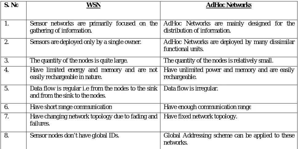
Table 1.2 WSN vs AdHoc Networks

S. No WSN AdHoc Networks

1. Sensor networks are primarily focused on the gathering of information.

AdHoc Networks are mainly designed for the distribution of information.

2. Sensors are deployed only by a single owner. AdHoc Networks are deployed by many dissimilar functional units.

3. The quantity of the nodes is quite large. The quantity of the nodes is relatively small. 4. Have limited energy and memory and are not

easily rechargeable in nature.

Have unlimited power and memory and are easily rechargeable.

5. Data flow is regular i.e from the nodes to the sink and from the sink to the nodes.

Data flow is irregular.

6. Have short range communication Have enough communication range 7. Have changing network topology due to fading and

failures.

Have fixed network topology.

8. Sensor nodes don’t have global IDs. Global Addressing scheme can be applied to these networks.

1.3 Architecture of WSNs [5]

WSN is a collection of the nodes that are thickly positioned either inside the target area in the environment or at a close proximity to it. Sensor networks are primarily focused on the gathering of information related to the environmental conditions. These networks are deployed in those areas where actual human interaction is almost impossible. These are the networks that have changing network topology due to failures and fading. Sensor networks are designed and developed in accordance with the requirements of the application for which they are to be used. As the gathering of data is based on a common phenomenon so the data collected by numerous sensors in WSNs is redundant in nature. The major components of a WSN are:

 Sensor Field: The area or the region of interest where the actual sensor nodes are deployed is known as sensor field. It can range from a small area to large cities. This is the quarter or the territory where the nodes are forever deployed. This is the rectangular field that surrounds the sensor nodes.

 Sensor Nodes: Sensor nodes form the essential part of the WSNs [5]. They are the basic component of the wireless sensor networks. These are the devices that are actually deployed in the field and they sense and amass the information from their environment and transmit it to BS where all the information from the sensor nodes is collected. This information can be used to recognize the prevailing environmental conditions in order to make decisions that are beneficial for the environment.

 Sink: This is a special type of sensor nodes which amasses, process and stores the information coming from the other sensor nodes in the network. The sink is called as the point of aggregation of data where the data from each node gets collected and processed. The total number of messages to be sent towards the BS is reduced by this node as it assembles the information from the nodes, summarizes the data which is further forwarded to the BS. The overall energy requirements of the wireless sensor network are minimized with the decline in the amount of messages to be sent to the BS.

(4)

ISSN(Online): 2320-9801

ISSN (Print): 2320-9798

International Journal of Innovative Research in Computer

and Communication Engineering

Fig 1.1 Architecture of Wireless Sensor Networks [5]

1.4 Hardware Components of Sensor Nodes

Each of the sensor nodes consists of five major components [5]. These are:

 Sensors: It consists of sensors which generate measurable reaction signals due to changes in environments like weather conditions, pressure, humidity and temperature. Analog signal sensed data are digitized by an analog-to-digital converter (ACD) and transferred to the embedded processor for additional processing. A sensor node can comprise of various sensors coordinated in or associated with the node. The primary objective for providing power supply for sensor nodes is to ensure that enough energy is made available to the nodes at the least cost, volume, weight, recharge time and longer lifespan.

 Central Processing Unit (CPU): The most important task of the CPU is to perform the processing of data and managing the various other hardware components of the sensor node. It is also responsible for performing the programming tasks.

 Power Supply: Energy expenditure in the sensor nodes is through the sensing of data, processing of data and communication. Power is more likely to be consumed by communication of data than when compared with data processing and also sensing data. Battery and capacitors act as storage facilities for power and then supply the power for the sensor nodes.

 Communication Unit (Transceiver): The transceiver is that part of the sensor node which is responsible for the actual wireless communication among the sensor nodes. There are four operational states of transceiver:

 Transmit: This is the state when the data is sent from one node to other nodes or from one node to the BS.

 Receive: This is the state of collection of the packets that are transmitted by other nodes.

 Idle: This is the state in which the transceiver is available to receive the packets but not ready to start receiving the packets.

 Sleep: In order to limit the ability of the transceiver to receive any data we prefer to switch off considerable sections of transceiver.

(5)

ISSN(Online): 2320-9801

ISSN (Print): 2320-9798

International Journal of Innovative Research in Computer

and Communication Engineering

Fig 1.2 Hardware Components of Sensor Node [5]

1.6 Types of Communication Models in WSN [7]

Every sensor node is identical in type of devices but the functionality provided by the sensor nodes differs with the type of the network structure. There are basic three types of communication system possible in the WSNs. The deployment of the sensor nodes, the power required for transmission, coverage and communication pattern used greatly affects the operations of the routing protocols at the node level as well as at the base station level. The protocols employed for routing in wireless sensor networks support three types of communication:

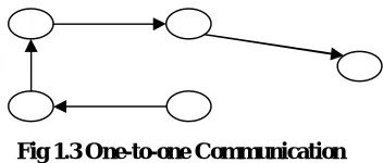
i) Uni-cast Communication (one-to-one): This type of communication pattern is used when there is communication between one node to the other node.

Fig 1.3 One-to-one Communication

ii) Multicast Communication (one-to-many): This type of communication pattern is used when the nodes wish to send their data towards the BS. The nodes in the field can communicate with the BS either directly by transferring their data to it or indirectly by sending their data to the neighbor node which further forwards it to the BS.

Fig 1.4 One-to-many Communication

iii) Reverse-multicast Communication (many-to-one): This type of communication pattern is used when the BS wants to send control information to the sensor nodes

BS SENSING SYSTEM

POWER SUPPLY SYSTEM

PROCESSING SYSTEM

COMMUNICATIO N SYSTEM

MEMORY SYSTEM Internal Sensors

(6)

ISSN(Online): 2320-9801

ISSN (Print): 2320-9798

International Journal of Innovative Research in Computer

and Communication Engineering

Fig 1.5 Many-to-one Communication

1.7 Challenges in WSNs[8]

Although the WSNs are similar more or less to the other networks but they face certain constraints and challenges which makes them different from the other networks. The various challenges faced in WSNs are:

 Limited Energy Capacity: The sensor nodes being small in size have limited energy to operate in the environment. These sensor nodes come with a small battery which needs to be charged or replaced in order to continue the functionality of the sensor. In case of some nodes both these option of charging or replacing the battery are not possible so the nodes die once they deplete all their energy. Due to limited energy they have limited survival time period. The main issue in WSN is how we can extend the network lifetime when the nodes have restricted energy limits. The main concern while designing a sensor network for an application is the energy efficiency which impacts the network to a great extent.

 Scalability: When the deployment of the nodes is done on a large scale, it not only provides redundancy as well as improves the fault tolerant capability but also raises scalability issue. The magnitude of nodes deployed within the network is dependent mainly on the importance value associated with the physical phenomenon. Thus the routing protocol needs to be designed as such that it is able to handle increased quantity of the nodes in the WSN.

 Production cost: The cost of a sensor node is also important while deployment of the nodes within the network. If the cost of a single sensor is quite higher than a traditional single sensor device than the cost of setting up the network would be considerably high. If the setup cost is large then the network will not be cost efficient.

 Transmission Media: The operation of the WSN relies heavily on the link with which the nodes are interconnected with each other. These links can be composed of radio, infrared, optical, acoustic links. In order to ensure that the network functions efficiently throughout the world it is important that the medium used is available everywhere in the world. Thus the transmission media plays a critical part in the profficient functioning of the WSNs and the transmission of information within the network becomes an important challenge in WSN.

1.8 Routing in WSNs

Routing refers to the process finding a path for sending as well as receiving the data between the source and the destination. The most important task performed in WSNs is to send as well as receive the collected information from the sensor field towards the BS. So the methods that are employed to transfer the data and information between source-target nodes become an important concern that ought to be tended to in the advancement of the WSNs.

Routing in WSNs is all the more difficult when contrasted to the early wireless networks due to their inherent feature of low power. First of all, as the wireless sensor networks have large quantity of nodes, that is why the routing protocols that are designed for these networks ought to be able to support the transfer of amassed data over long distances, without getting concerned about the size of the network. Another important thing to be noticed in wireless sensor networks is that a certain quantity of the functioning nodes may fall short during the network operation just because of the diminution of energy of the sensor nodes, breakdown of internal hardware or various other physical factors. This issue should not interfere with the typical functioning of the network. Furthermore, as the sensor nodes have restricted power supply, lesser capability to process the data, lower memory limit and available bandwidth, so information distribution should be performed with effective utilization of the network resources. Furthermore, as the performance of the WSNs is totally dependent upon the type of the application, so the routing protocols designed ought to be able to satisfy the Quality of Service requirements of the application. [9]

(7)

ISSN(Online): 2320-9801

ISSN (Print): 2320-9798

International Journal of Innovative Research in Computer

and Communication Engineering

The locations of sensor nodes are static and the BS knows them all in advance. The sensor nodes can exchange and in addition get the information from the BS either straightforwardly or by means of some other sensor nodes. These nodes periodically sense the data from the environment surrounding them and they always have some type of information for sending in every round of transmission of data. The nodes combine and aggregate their data with the data they have received from the other nodes, and turn out just one packet of data without being concerned about the number of packets of data received by them. The major issue is to find an efficient routing technique to transfer the packets of data collected from the sensor nodes towards the BS, in an energy efficient manner [10].

1.9 Routing Techniques in WSN [10]

Routing is a process of shaping a path between source and destination for sending as well as receiving the data upon request for data transmission. It involves the process of transferring the information from the nodes to the BS, where this information is collected and analyzed in order to help in the decision making process. There are different types of architecture involved in routing the information from the nodes to the BS which are described as follows:

 Single Hop Routing: The earliest & simplest methodology was immediate transmission of the data. In this approach each of the sensor node would detect & transfer its data to the BS directly without the assistance of any intermediate node. As the BS is sited at a distance from the sensor nodes, it brings about expanded expense of transmission of the information, due to which the energy of the nodes depletes faster & in this way the sensor nodes have short network lifetime.

Fig 1.6 Single Hop Routing

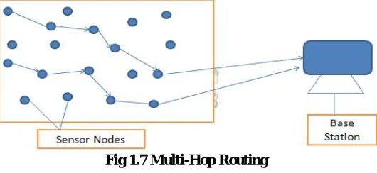
 Multi-Hop Routing: In this, each of the sensor nodes transmit its data to its immediate neighbor, and with multiple hops the data from the neighbor node are transferred to the BS. In multi-hop networks, each node consumes less energy for transmitting their data as compared to Single-hop. Multi-hop wireless sensor network is more efficient then single-hop network. In real world observations, single-hop network is more efficient then multi-hop because in single-hop lower packet loss. In this architecture, the nodes closer to base station have more load on them so they drain off their energy faster as compared to other nodes which effects the network lifetime.

Fig 1.7 Multi-Hop Routing

1.10 Routing Protocol Design Challenges [11]

(8)

ISSN(Online): 2320-9801

ISSN (Print): 2320-9798

International Journal of Innovative Research in Computer

and Communication Engineering

o Limited Energy Capacity: The sensor nodes in wireless sensor networks come outfitted with small, non-rechargeable batteries so these nodes have limited energy capacity. Sometimes the sensor nodes are placed in certain areas where it becomes impossible to supplant the batteries. In these circumstances when the sensor nodes do not have a wellspring of energy to work, so they won't have the capacity to work legitimately. They will not function properly because their energy crosses certain threshold value which will further affect the network performance. Thus routing protocols should be energy efficient in nature in order to improve the network lifetime as well as increase the network performance.

o Inadequate hardware resources: Due to limited processing and stockpiling limits of the sensor nodes, these nodes can perform only limited computational functionalities. The hardware constraints as limited memory, low storage and processing capability of the sensor nodes in the WSNs thus present many difficulties in the outline and development of the routing protocols.

o Random and massive deployment of sensor nodes: Sensor nodes in WSNs can be deployed either manually or randomly due to their application dependent nature which affects the network performance. Thus the sensor nodes deployment should be as such to enable energy efficient network operations.

o Data aggregation: While transmitting the data towards the BS, the sensor nodes generate huge amount of redundant information. Keeping in mind the end goal to evacuate the repetitive information and to lessen the aggregate number of messages to be sent, the only way possible is to aggregate the data coming from multiple nodes into one single packet and transmit it to the BS. This technique of data aggregation has been utilized as a part of various routing protocols to achieve energy efficiency.

o Scalability: Routing protocols ought to have the capacity to scale with the system size.

1.11 Applications of WSNs [12]

o Area Monitoring

o Healthcare Monitoring

o Habitat Monitoring

o Monitoring of pollution present in air

o Detection of forest fire

o Detection of landslides in particular areas.

o Measuring the quality of water

o Prevention of natural disaster

o Industrial Monitoring

1.12 Advantages of WSN [12]

o Network setups can be done without the need of any fixed infrastructure.

o These networks are ideal for the places where it is not easy for a human being to reach like underwater, on high mountains or dense forests.

o Flexible in nature i.e they can easily adapt to any change that occurs in their surroundings.

o The cost of implementation is quite low as compared to other network.

1.13 Disadvantages of WSNs [12]

o As the hackers can easily gain access to these networks and hack all the information so these networks are less secure in nature as compared to other networks.

o Wireless sensor networks have lower speed when contrasted with a wired network.

o WSN are more perplexing to plan than a wired framework.

o WSNs are effectively influenced by their surroundings.

o Energy constraint in case of sensor nodes presents a great challenge for the wireless sensor network.

II. RELATED WORK

(9)

ISSN(Online): 2320-9801

ISSN (Print): 2320-9798

International Journal of Innovative Research in Computer

and Communication Engineering

to the BS. Each node takes turn in becoming the CH and transferring the data to the BS. One of the most important clustering based protocols is LEACH

LEACH is a versatile cluster-based protocol that randomly distributes the load equally between the nodes in the network [13]. The key idea of this protocol is to decrease the total quantity of the sensor nodes that send as well as receive the data individually to and from the BS i.e these nodes sense the information related to a specific process from their environment and then send that information to the BS on their own where it the information received is used for decision making process. In order to achieve the desired goal, this protocol forms small clusters and each cluster contains a head node called the cluster head (CH). The CH is in-charge of collecting the information from cluster nodes, then summarizing the collected data and sending the aggregated results to the BS. LEACH also makes use of the concept of randomization for CH determination and accomplishes up to 8x change when contrasted to the immediate transmission approach. The amount of the data transmitted to the BS is also reduced. The cluster head are selected randomly but each node gets the chance to become CH. A threshold t(n) is fixed first for cluster head selection

( ) =

1− ∗ 1

, ∈

Here the percentage of the sensor nodes that can become CHs is represented by P, the round number is denoted by r; the set of the sensor nodes that have not become CHs in last 1/P rounds is represented by G. The node n randomly chooses a value lying between 0 and 1.

For a node n to become the CH, the value of the random number chosen by the node should be less than the value of the threshold t(n). If the value of the random number is greater than the threshold value, then a node cannot become CH in the present round. Along with the advantages provided, there are certain disadvantages of LEACH. These are: 1. Cost of forming the clusters is very high.

2. Several CHs transfer the amassed and aggregated data to the BS placed at a distant location which increases the energy cost for data gathering.

To overcome these disadvantages PEGASIS protocol was introduced.

PEGASIS [14] was introduced as an improvement over LEACH as the key idea in PEGASIS is to connect the sensor nodes using a chain of shortest length. The nodes can construct the chain either themselves using Greedy Algorithm or the BS computes the chain for the nodes and broadcasts the information to the nodes. This protocol follows a token passing approach in which one node that is designated as the leader node passes a small size token starting from the end nodes to transmit the data. This token passes from node to node and in this way gathered information will move from node to node, get fused with the data of the receiving node that possesses the token, and eventually reach a node designated to transfer this fused data to the BS. Information combination is performed at all the nodes except the end nodes. In order to reduce the average energy that each node spends per round, the nodes take turn in transmitting the data to the BS. This provides an improvement over LEACH as in this protocol just one node transmits the data to the BS instead of several cluster heads per round. This improvement reduces the energy cost for data fusion and transmission.

PEDAP [15] protocol is further extension of PEGASIS protocol. The PEGASIS protocol connects each of the sensor nodes using a chain with the most limited length while in the PEDAP protocol, each of the sensor nodes are connected to each other through a minimum spanning tree. PEDAP protocol expects that the locations of all the sensor nodes are known by the BS in advance. The route for transfering the information from the nodes to the BS is calculated with the help of Prim’s minimum spanning tree algorithm in which the BS becomes the root of the tree. The base station removes the dead nodes after regular interval of time and again computes the routing information and forwards it to the node which requires it. Thus PEDAP protocol dissipates less energy than the other two protocols. The drawback of PEGASIS is that the nodes which are placed at a large distance from the BS on the chain suffer from excessive delay in the transfer of their data to the BS [16].

(10)

ISSN(Online): 2320-9801

ISSN (Print): 2320-9798

International Journal of Innovative Research in Computer

and Communication Engineering

the next tier begin sending the summarized information to the BS. Furthermore, when the energy of the last tier goes beneath the edge level then a new threshold is defined. This process of redefining the threshold is repeated until the threshold becomes less than the dead energy of the nodes.

Minimum Spanning based Clustering Tier Technique (MSCT2) [18] is an improvement of MSMTP protocol. An improvement is made in the MSMTP protocol by introducing the concept of clusters within the tiers which will further increase the system lifetime. In this the cluster heads of the same tier are connected to each other as well as the other tier cluster heads using MST. By using this arrangement lesser number of nodes is used in the transmission of amassed data to the BS.

In the proposed work the whole network is segmented into 3 tiers according to the distance of the nodes from the BS. Each tier contains fixed number of clusters i.e one cluster in Tier 1, two clusters in Tier 2 and 4 clusters in Tier 3. The nodes are allocated tier IDs and cluster IDs at the initial setup stage. Clusters are formed using the Minimum spanning tree (MST) approach. In [17,18] authors proposed a scheme in which, each tier contains clusters and the data was transmitted first between the CHs of the same tier which were connected to each other through a MST and then the data was forwarded to the next tier by the one of the CH of the previous tier. This arrangement increased the load on a single CH that was connected via MST to the next tier, as all the clusters send their data to this cluster head which then forwarded their data to the next tier. In order to improve this situation it is required that any cluster which wants to send data to the other tier be connected with the other tier directly through MST so that it could transmit its data to the next tier CH nearest to it. In this way the transmission cost is reduced. This requirement is fulfilled in the proposed work. The protocol is named as Tier Based Minimum Spanning Tree Structured Protocol (TBMSTP).

III. THE SYSTEM MODEL

A. Network Model [7]

The protocol assumes that 100 sensor nodes are distributed randomly in the network area of diameter 100m. Notwithstanding information collection, every node of the system has the capacity to send the information to other sensor nodes and in addition to BS. The point is to transmit the amassed information to base station with least loss of energy which in fact increases system life time. The proposed work considers a sensor network environment where: • Each node senses the information from its environment and forwards the collected information to the BS.

• BS is placed in the center of the field.

• Sensor nodes are homogeneous & energy constrained. • Sensor nodes are stationary & are uniquely identified.

• Information combination & collection is utilized to lessen the size of message in the system.

B. Radio Model

Based on energy level used in [13], we have:

Where l is the number of transmitted bits, Eelec is the energy consumption to run the transmitter or receiver. Eamp or Efs

depends on do.

In the simulation, a packet length k of 2000 bits is considered. C. Problem Statement

The main challenge faced in WSN is to maximize the lifetime of the network. The proposed work is focused on finding a routing scheme that is capable of delivering the collected information from sensor nodes to the BS in an energy efficient manner. The lifetime of the system is the time passed until a large portion of the nodes or some predefined part of the nodes become dead. The time in rounds where the last node drains the greater part of its energy characterizes the lifetime of the general sensor system. Taking these different possible requirements into consideration, proposed work provides the timings of the death of every node.















4 2

*

)

,

(

d

l

E

d

l

E

d

l

E

mp elec fs elec Tx



d  do

(11)

ISSN(Online): 2320-9801

ISSN (Print): 2320-9798

International Journal of Innovative Research in Computer

and Communication Engineering

IV. PROTOCOL DESCRIPTION

TBMSTP segments all the nodes into three unique tiers, according to their remoteness from the BS. The framework dispenses a tier ID and cluster ID to every node in the midst of the instating stage. The sensor nodes that have the same tier ID are supposed to be placed in the same tier. The sensor nodes belonging to the same tier are placed at same distance from the BS, and use the same amount of energy for transferring information to the BS. Lower tier IDs are allocated to the nodes that are situated closer to the BS.

Each tier contains different number of clusters. We have taken one cluster in the Tier 1, two clusters in Tier 2 and four clusters in Tier 3. The tier partitioning is done in the following manner:

Tier1 = Distance of the node from BS is upto 15m

Tier2= Distance of the nodes from the BS is greater than equal to 15m to less than 35m Tier3= Distance of the nodes from the BS is greater than 35m

Clusters are formed within the tier where member nodes are connected to the CHs with the help of Minimum Spanning Tree (MST). A Spanning Prim’s Algorithm is used for the MST construction between the nodes and CHs as well as between CHs of different tiers. A spanning tree of a graph is a connected sub-graph in which there are no cycles. The minimum spanning tree for a given graph is a minimum cost spanning tree for that graph.

The distance of one node from each of the nodes in the network is calculated. This distance is assigned as weights of the edges connecting a node to each node in the network. Adjacency matrix is formed containing the distance of one from the other nodes in the field. This adjacency matrix is taken as input in the Prim’s algorithm for calculating the minimum weighted spanning tree. MST is used for calculating the cost incurred to send as well as receive the collected information from the nodes to the BS and vice-versa. The path constructed by MST is used for transmission of data to the BS with minimum cost and in turn increasing the stability period of the network.

Data Transmission

In TBMSTP, each of the sensor node advances its collected and aggregated data to the CH to which it is connected in MST structure. Then the CH of topmost rank tier will send the summative data of the nodes of the cluster to the nearest CH in the next tier and finally to the BS. CH of the first tier i.e Tier 1 will continue to send the summarized information to the BS till all the nodes of first tier have the energy which is higher than the threshold level defined for the nodes. When the energy of the nodes of the first tier goes below the threshold level then the CH of the second nearest tier i.e Tier 2 will begin to transmit the amassed data towards the BS and the same course of action will be repeated with the nodes of third tier i.e Tier 3 which is located at a significant distance from the BS. This procedure of shifting the power to send the information from the nodes to the BS taking turns is known as SHIFTING OF THE TOP TIER [17]. In this procedure when all the nodes of a single tier becomes dead then the nodes of the next nearest tier begin to transmit the amassed information to the BS [17]. When all the nodes of the end tier i.e Tier 3 have their energy less than the target energy level then a new target level of energy is set. This process continues till the threshold goes below the dead energy. At this point the complete network is assumed to be dead as all the nodes forming the network become dead.

(12)

ISSN(Online): 2320-9801

ISSN (Print): 2320-9798

International Journal of Innovative Research in Computer

and Communication Engineering

V. RESULTS

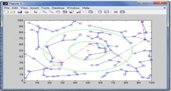
For evaluating the performance of the proposed protocol, the simulation is carried out on the network of 100 nodes. The simulations are done in MATLAB. The BS is placed at (50, 50) in a field of 100m x100m. Simulation is done in order to determine the round in which every node becomes dead. Parameters used are shown in the table below.

Table 1. Parameters Used

Parameters Value

Electronics energy (Eelec ) 50 nJ/bit

Energy for data aggregation (EDA) 5 nJ/bit/signal

Initial energy of sensor node (Einit ) 0.25J,0.5J & 1J

Communication energy (Efs) 10 pJ/bit/m2 Communication energy (Emp) 0.0013 pJ/bit/m4

Threshold value of distance (d0) 75m

Sensing Area (M x M) 100x100 Number of nodes 100 Base Station 50x50

A node once dead is considered dead for the rest of simulation, and the results show vastly improved system stable lifetime(period when all nodes of network are alive) because it balances energy dissipation among sensor thus maximizing stable life time & accomplishes preferred results over other protocols aside from PEDAP

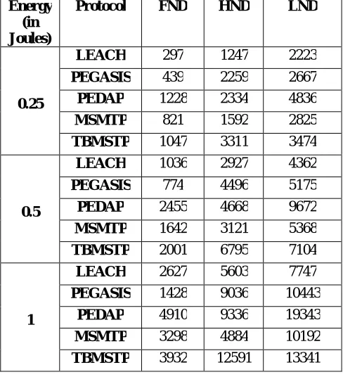
Table 2. Timing of death of nodes in terms of round number where Base Station is at the center [7]

Energy (in Joules)

Protocol FND HND LND

0.25

LEACH 297 1247 2223

PEGASIS 439 2259 2667

PEDAP 1228 2334 4836

MSMTP 821 1592 2825

TBMSTP 1047 3311 3474

0.5

LEACH 1036 2927 4362

PEGASIS 774 4496 5175

PEDAP 2455 4668 9672

MSMTP 1642 3121 5368

TBMSTP 2001 6795 7104

1

LEACH 2627 5603 7747

PEGASIS 1428 9036 10443

PEDAP 4910 9336 19343

MSMTP 3298 4884 10192

(13)

ISSN(Online): 2320-9801

ISSN (Print): 2320-9798

International Journal of Innovative Research in Computer

and Communication Engineering

Table 2 summarizes the results for base station located at the center of the field. A the table shows the lifetime of the network improve as compared to LEACH, PEGASIS and MSMTP protocols. Here FND stands for first node dead, HND stands for half node dead and LND stands for last node dead. Results for the previous protocols were referred from [7]

Fig 5 Comparison between various protocols to check the lifetime of the network

Figure 5 shows the comparison graph between various protocols when the BS is sited at the middle of the sensor field and nodes are deployed with 0.5J as the initial energy and shows the scenario when the first, half and last node of the system becomes dead. The results demonstrate that TBMSTP performs better than the previously proposed protocols i.e LEACH, PEGASIS and MSMTP protocols. With some changes in the routing technique the network lifetime can be improved considerably.

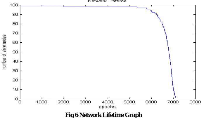
Fig 6 Network Lifetime Graph

(14)

ISSN(Online): 2320-9801

ISSN (Print): 2320-9798

International Journal of Innovative Research in Computer

and Communication Engineering

Fig 7 represents a plot between the packet delivery ratio and the rounds when initial energy of the nodes is 0.25J. The PDR is the ratio of the number of packets of data that are successfully delivered to the destination in comparison to the number of packets of data that are sent by the sender.

Fig 7 Packet Delivery Ratio vs Epochs when initial energy=0.25J

The greater value of PDR indicates better performance of the given protocol. The value of PDR is constant until all the nodes in the network survive. When the nodes in the network starts becoming dead the PDR starts decreasing i.e the packet received are getting lesser than the packets sent. This leads to loss of packets. As is seen from the fig 5.7, there is no packet loss until the all nodes are alive. The PDR starts decreasing as the first node in the network becomes dead i.e at 1047, and goes on decreasing gradually as the nodes become dead.

Fig 8 represents a plot of the timings in terms of round number when every node in the network becomes dead. The x-axis represents the node number and y-x-axis represents the round number. The red colored bar represent the time when the node becomes dead. For example as in the table above the first node, when the initial energy is 0.25J, becomes dead at round number 1047. The red bar at first node goes beyond round number 1000 at extends up to 1047. Similarly all the nodes with their timings of death are shown in this figure.

Fig 8 Timings of death of each node w.r.t time in terms of rounds at energy level=0.25J 0

1000 2000 3000 4000

1 8 15 22 29 36 43 50 57 64 71 78 85 92 99

R

o

u

n

d

s

(15)

ISSN(Online): 2320-9801

ISSN (Print): 2320-9798

International Journal of Innovative Research in Computer

and Communication Engineering

Fig 9 Comparison of Stability period of Previous vs Proposed protocol at Einit=0.25, 0.5, 1J

Fig 9 shows a plot showing the comparison of stability period of previous protocols vs proposed protocol. Stability period is referred to as the duration of the network operation from the start till the first node dies. From the above plot it is clear that the proposed protocol i.e TBMSTP provides a much stable system lifetime as compared to LEACH, PEGASIS & MSMTP protocols.

VI. CONCLUSION

In this paper a new routing strategy has been proposed. This strategy is based on the concept of Tier i.e partition the network into parts and Minimum Spanning Tree (MST) construction technique. Thus this protocol is called as TBMSTP (Tier Based Minimum Spanning Tree Protocol). Through our study and simulation of the proposed work we conclude that the system’s stable lifetime is improved than the existing routing protocols. This protocol contributes a lot towards prolonging the network lifetime.

REFERENCES

1. Li, Changle, et al. "A survey on routing protocols for large-scale wireless sensor networks." Sensors 11.4 (2011): 3498-3526.

2. Nikolidakis, Stefanos A., et al. "Energy efficient routing in wireless sensor networks through balanced clustering." Algorithms 6.1 (2013): 29-42. 3. Akkaya, Kemal, and Mohamed Younis. "A survey on routing protocols for wireless sensor networks." Ad hoc networks 3.3 (2005): 325-349.

4. Jadhav, Meera. "Clustering Based Energy Efficient Protocols For Wireless Sensor Networks."International Journal Of Engineering And Computer Science 3.3 (2014): 5177-5184.

5. Almazroi, Abdulaleem Ali and Ngadi Ma. “A Review On Wireless Sensor Networks Routing Protocol: Challenges In Multipath Techniques”, Journal of Theoretical and Applied Information Technology 59.29(2014): 469-509

6. Chong, Chee-Yee, and Srikanta P. Kumar. "Sensor networks: evolution, opportunities, and challenges." Proceedings of the IEEE 91.8 (2003): 1247-1256. 7. Pantazis, Nikolaos, Stefanos A. Nikolidakis, and Dimitrios D. Vergados. "Energy-efficient routing protocols in wireless sensor networks: A

survey."Communications Surveys & Tutorials, IEEE 15.2 (2013): 551-591.

8. Akyildiz, Ian F., et al. "Wireless sensor networks: a survey." Computer networks 38.4 (2002): 393-422.

9. Radi, Marjan et al. “Multipath Routing in Wireless Sensor Networks: Survey and Research Challenges.” Sensors 12.12 (2012): 650–685.

10. Bathla, Gaurav, and Gulista Khan. "Energy-efficient Routing Protocol for Homogeneous Wireless Sensor Networks." International Journal on Cloud Computing: Services and Architecture (IJCCSA) 1.1 (2011): 12-20.

11. Singh, Shio Kumar, M. P. Singh, and D. K. Singh. "Routing protocols in wireless sensor networks–A survey." International Journal of Computer Science & Engineering Survey (IJCSES) 1.2 (2010): 63-83.

12. Bhattacharyya, Debnath, Tai-hoon Kim, and Subhajit Pal. "A comparative study of wireless sensor networks and their routing protocols." Sensors 10.12 (2010): 10506-10523.

13. Heinzelman, Wendi Rabiner, Anantha Chandrakasan, and Hari Balakrishnan. "Energy-efficient communication protocol for wireless microsensor networks."System sciences, 2000. Proceedings of the 33rd annual Hawaii international conference on. IEEE, (2000):3005 – 3014.

14. Lindsey, Stephanie, and Cauligi S. Raghavendra. "PEGASIS: Power-efficient gathering in sensor information systems." Aerospace conference proceedings, 2002. IEEE. Vol. 3( 2002): 924-955.

15. Tan, Hüseyin Özgür, and Ibrahim Körpeoǧlu. "Power efficient data gathering and aggregation in wireless sensor networks."ACM Sigmod Record 32.4 (2003): 66-71.

16. Singhal, Vishakha, and Shrutika Suri. "Comparative Study of Hierarchical Routing Protocols in Wireless Sensor Networks." International Journal of Computer Sciences and Engineering 2.5 (2014): 142-147.

17. Khan, Gulista, Gaurav Bathla, and Wajid Ali. "Minimum Spanning Tree based Routing Strategy for Homogeneous WSN." International Journal on Cloud Computing: Services and Architecture(IJCCSA)1.2(2011): 22-29.