Article
Soil
and
Crop/Tree
Segmentation
from
Remotely
Sensed
Data
by
U
sing
Digital
Surface
Models
Adriano Mancini†, Jack Dyson†, Emanuele Frontoni†∗and Primo Zingaretti†
* Correspondence: [email protected]
† Dipartimento di Ingegneria dell’Informazione, Università Politecnica delle Marche, Ancona, ITALY
Abstract:The increased availability of high resolution remote sensor data for precision agriculture
1
applications permits users to aquire deeper and more relevant knowledge about crops states that lead
2
inevitably to better decisions. The algorithm libraries being developed and evolved around these
3
applications rely on multi-spectral or hyper-spectral data acquired by using manned or unmanned
4
platforms. The current state of the art makes thorough use of vegetational indicies to guide the
5
operational management of agricultural land plots. One of the most challenging sub-problems is
6
to correctly identify and separate crop from soil. Thresholding techniques based on Normalized
7
Difference Vegetation Index (NDVI) or other such similar metrics have the advantage of being simple,
8
easy to read transformations of the data packed with useful information. Obvious difficulties arise
9
when crop/tree and soil have similar spectral responses as in case of grass filled areas in vineyards.
10
In this case grass and canopy are close in terms of NDVI values and thresholding techniques will
11
generally fail. Radiometric approaches could be integrated or replaced by a geometric approach that
12
is based on terrain data like Digital Surface Models (DSMs). These models are one of the ouputs
13
of orthorectification engines usually present in data acquired by using unmanned platforms. In
14
this paper we present two approaches based on DSM that are able to segment crop/tree from soil
15
while over gradient terrain. The DSM data are processed through a two dimensional data slicing or
16
reduction technique. Each slice is separately processed as a one dimensional time series to derive the
17
terrain and tree structures separately, here interpreted as object probability densities. In particular
18
the first approach is a Cartesian grid rasterization (CARSCAN) of the terrain and the second is its
19
immediate generalisation or radial grid rasterization of the DSM model (FANSCAN). The FANSCAN
20
recovers information from the original image at greater frequencies on the Fourier plane. These
21
approaches enable the identification of crop/tree from soil in case of slopes or hilly terrain without
22
any constraint on the displacement / direction of plant/tree row. The proposed algorithm uses pure
23
DSM information even if it is possible to fuse its output with other classifiers.
24
Keywords:Segmentation; multi-spectral camera; soil: tree; raster scanning; UAV application
25
1. Introduction 26
The acquisition of high resolution imagery for precision agriculture applications is a common task
27
for a large variety of users as agronomists, big-data specialists and researchers. Unmanned system
28
are able to capture data with ultra high resolution (up to 1 cm of terrain) also by using multi-spectral
29
or hyper-spectral payloads. Typically data are acquired by a large set of overlapping images that are
30
post-processed to derive a single global ortho-photo of the region of interest. The main advantages
31
of such platforms is data aquisition in presence of cloud overlay which a satellite cannot do. On the
32
contrary the cost of surveying can increase despite the availablility several low cost flight platforms
33
and payloads [1]. In this new high-resolution era, due in part to Unmanned Aerial Systems (UASs)
34
[2], opens new ways to analyze the fields, crops and trees during the growing process for proper
35
management of all operations (e.g. applied, tilling,. . . ) in order to maximize yield, quality and
36
optimize costs [3]. In this sense, UAS platforms stand ready to overcome the main limitations of
37
satellite platforms, ensuring very high resolution spectral, spatio-temporal data aquisition systems [4].
38
In this scenario, the data play a key role in feature extraction where the manipulation of spectral bands
39
is the classical methodological tool to start an analysis - possibly as an input feed to other methods for
40
further analysis. Vegetational indices are usually used in a context where machine leaning algorithms
41
are used to classify data in both pixel and object domains [5]. These become more effective if they are
42
given access to a proper feature set at the start of their analysis runs. The planning of task (e.g., variable
43
rate) requires a deep knowledge of crops and their status [6]. The classical output of an analysis from
44
an expert is a prescription map that will map tractor operations like spraying or treatment application
45
over the field. The generation of a prescription map requires the definition of management zones
46
that reflect areas and their status [7]. The typical case is variable rate Nitrogen fertilizer application
47
as discussed in [8]. The generation of management zones and their prescription maps may then be
48
automated starting from decision support systems that fuse heterogeneous data as well the soil signal
49
and the previous yield together with the vegetation indices [9,10].
50
When performing an analysis based on vegetation indices, it is important to consider only data
51
relevant to the problem. Here by the term relevant we mean pixels related to crop or tree field without
52
considering the soil variation. In this case the segmentation of soil and crop or tree field has a strong
53
impact on the evaluation of region of interest. The segmentation process of crop and tree vs soil could
54
be considered as an advanced Land Use or Land Cover mapping. The identification of crops could be
55
carried out by using spectral or spatial or indeed both features. Spectral segmentation usually relies
56
on supervised or unsupervised algorithms also including the use of satellite data [11]. One of the
57
important requirements, as mentioned above, is that both soil and crops must have a different spectral
58
signature. When GSD are of the order of 1−2 meters a lot of ground noise is mapped into the pixels
59
and the result is that the underlying soil response could be influenced by the crop sgnal just above it.
60
In this case it is necessary to increase the resolution and UAS platforms are the suitable systems to
61
gather these data.
62
High resolution images can cause further problems through the data intrinsic noise signals. An image
63
with a 1 centimeter GSD is quite challenging to analyze considering the high variability of crop and soil
64
signals. In this case other than pure spectral features, the spatial and geometric features become useful
65
in order to extract further information about the ground truth probability distribution in the data. In
66
particular, the crop height field is an important but simple mathematical variable to indicate crop vs
67
soil signal rations. It can also act as a sensor able to measure crop’s growth [12]. Volume estimation is
68
also possible and this represents and additional variable to use in the decision making process [13].
69
Synthetic Aperture RADAR (SAR) can also be used to retrieve agricultural crop height from the
70
event space even if the resolution and cost are challenging [14]. A viable solution is the use of UAS
71
platforms that are able to measure height by direct and indirect methods. Such systems are able to
72
host compact multi-spectral and hyper-spectral sensors [15] acquiring images that are orthorectified
73
by using approach as Structure from Motion (SfM) that is a part of the overall processing pipeline [16].
74
The quantification and identification of soil and vegetation is important for several purposes [17] as an
75
estimator for growth [18,19], 3D monitoring [20] and weed identification [21,22]. The identification of
76
weeds is important to ensure uniform growth of the target crop [23] and is also supported by methods
77
able to classify crops, weeds and their foundation soils [24] through the use of Excess Green Index
78
(ExG) [25].
79
Vineyards and fruit plants are a typical example of complex regions in both detection and study. Slope
80
in the terrain and also the presence of grassed soil substantially influence the overall terrain statistics.
81
Detection can be carried out by using algorithms based on frequency analysis [26], Hough Space
82
Clustering or Total Least Squares as in [27].
In this paper we propose a novel method named FANSCAN that extend our previous methods [28]
84
(also CARSCAN) to segment canopy/tree coverage vs the underlying soil. The segmented image
85
is fundamental to correctly performing an analysis that requires the exact knowledge of the canopy
86
position. FANSCAN is also related to our previous research to extract objects from complex data-set as
87
the case of Lidar-Multispectral as described in [29,30]. Previous work proposed a slicing approach
88
that fuses adaptive thresholding and 1D scan of the images. The FANSCAN approach instead tries to
89
improve the segmentation also in case of heterogeneous fields with tree / crops displaces over several
90
directions.
91
The CARSCAN and FANSCAN rely only on Digital Surface Model (DSM) of the study area. This is
92
not an hard constraint considering that orthorectification engines produce orthophoto, dense cloud
93
and also DSM. However it is possible to integrate the results of the above mentioned approaches with
94
others based on radiometric classification.
95
The paper is structured as it follows. Section2presents the proposed approaches. Section3presents
96
the results of CARSCAN and FANSCAN on two data-set in Section4the conclusions and future works
97
are outlined.
98
2. Methodology 99
The correct tree and crop segmentation plays a key role in the domain of precision agriculture as
100
outlined in Section1. In this paper we outline and develop algorithms based on pure terrain based
101
features and if possible their subsequent fusion with pure spectral approaches as in [28].
102
Radiometric and spectral features derived from multi/hyper-spectral images can be used by
103
unsupervised or supervised algorithms to classify data and then select only the classes of interest
104
to evaluate the vegetation status. Unsupervised algorithms (e.g., hierarchical clustering, ISODATA,
105
k-means) require that the area contains objects (e.g., tree, crop, soil) that are spectrally separable. Soil
106
response in the presence of grass could produce incorrect results considering the spectral response
107
of bare soil with respect to one grassed over. A standard thresholding algorithm usually fails when
108
applied to the grassed over terrain problem due to a reduction in the crop to soil area signal to noise
109
ratio. As has already been mentioned, the presence of grass on the ground therefore strongly influences
110
the accuracy of classification. Supervised algorithms, if properly trained are able to capture grassed
111
soil, bare soil and tree/canopy but a common problem is the definition of a precise training set that
112
will not underfit the problem. This requires a photo-interpretation of the area and the typical use-case
113
for precision agriculture are small areas (from 1−1000 hectares). A reliable training set is usually
114
defined by a human user that should take into account local variability including spurious areas like
115
shadows [31].
116
To get around this, one can use information inherent in the data itself. In this second approach, soil
117
and tree detection is carried out by using purely mathematical features of the height field in the DSM
118
obtained during the orthophoto generation. The effectiveness of this technology depends strongly
119
on the scanning technique used. We investigate this dependency in detail by using a Cartesian grid
120
scanning method to compare to a radial scanning technique over the image coordinate space. The
121
results are theoretically connected to the object Fourier transform and this relationship is used to
122
develop a quality index for comparing the two types of scan.
123
This type of analysis provides a powerful basis for precision agriculture applications that require an
124
accurate and precise detection of crops in order to properly support decisions based on vegetational
125
indexes that must be evaluated only on not soil areas.
126
The pure radiometric approach becomes challenging when the spectral response of canopy is close to
127
the soil response. This is indeed the case for vineyards and fruit plants where the soil can be with or
128
without grass overlay.
2.1. One dimensional rasterization theory 130
The DSM is the output of an orthorectification engine that processes high-resolution images (with a
131
typical GSD in the 10−50 centimeter range). Many land areas are covered by foliage and trees,τ, 132
which obscure the underlying terrain or soil signalσ. The overall image signal is the algebraic sum of 133
these two quantities:
134
y(x,z) =τ(x,z) +σ(x,z) (1)
Each signal is a valuable source of information and it is useful in the context of object detection to be
135
able to separate them efficiently and accurately. For a test image like the one in Figure1, we develop a
136
simple and general mathematical procedure that separates the soil and tree signals into two separate
137
digital vector fields.
138
The combined terrain and foliage signalyis raster scanned (see Figure1) along a coordinate direction
139
such asz. Separating out the original surfacehinto a series of sample points in thez-direction obtains
140
a set of ’unrelated’ one dimensional images ready to be processed independently.
141
Taking an arbitrary sectionz=const across the image in Figure1one can reduce the soil extraction
142
problem into a series of one dimensional sub-problems which are in theory at least, easier and faster to
143
process.
144
Therefore, at some fixedz:
145
y(x) =τ(x) +σ(x) (2)
whereτandσare the tree and soil fields across some givenz-coordinate respectively. 146
The functionyis never inC1(the set of all one-fold differentiable functions). Therefore, differential
147
methods are not general enough without significant pre-processing and a potential loss of data. The
148
digital nature of the data does however permit the use of efficient set filters designed to separate a
149
slow digital derivative from a relatively fast one. We will show below that this observation can be
150
linked to statistical integral methods for solving the general problem.
151
One might argue that Fourier methods are also relevant here. They can be for specific cases. However,
152
the instability of the FFT when the signal is contaminated with any significant level of noise outweighs
153
any potential advantage a low pass filter would have. The main reason is that any attempt to control
154
noise through expedients like Weiner or spectral filters will tend to remove high frequency detail from
155
the image ad-lib, rendering the quickly-varying tree or contoured terrain signals inaccurate or even
156
omitting them completely. We will show below that the use of a direct method can recover information
157
from the Fourier space in a non-destructive fashion.
158
As already hinted above a more stable method is to use statistics: trees on the ground can be defined
159
by their scatter probability densityp(x, z)function. The importance of this function is in defining
160
the nearest neighbor distance from any given point(x, z). Idealizing, at some such point, the tree
161
population probability density function maximizes locally over some differential(x+dx, z+dz). The
162
associated probability density maximum is therefore constrained over some nearest neighbor contour
163
on thexz-plane:
164
∇p(x,z)·d(x,z) =0 (3)
The nearest neighbor (generally non-differentiable) probability contour serves to define a correlation
165
distance or integral of a tree or other object classτto its nearest neighbors. Every point on the nearest 166
neighbor contour will tend to satisfy a maximum of this correlation integral:
167
0=d
Z Z
τ x0, z0τ x0+x, z0+zdx0dz0
(4)
In the one dimensional language of Figure3this equation simplifies to:
0= Z
τ x0dτ dx x
0+x
dx0 (5)
over the object separation w. In other words, when this integral is at a stationary maximum, it
169
corresponds to a local probability maximum in one dimension which dictates the local distancewto a
170
nearest neighbor for the object classτ. The local spatial frequency of the object classτat the pointxis: 171
ωx= 2 π
w (6)
and corresponds to the Fourier or correlation frequency of the object classτembedded into the signal 172
y. The frequency distribution of object classes on the ground gives rise to a curious relative symmetry:
173
when the solution of equation3is a correlation minimum, from equation2, the cross-correlation
174
function of the soil will be a maximum instead:
175
Z y x0
τ x0+xdx0= Z
σ x0τ x0+xdx0 (7)
At such points y is a local minimum since there is no object field, by replacing τ(x0+x) with a 176
normalised windowkof integration widthw:
177
σ(x,w) =ymin<cR y(x0)k(x0+x)dx0=
R
y(x0)τ(x0+x)dx0 (8)
for some constantc. If the integration window width is made equal to the correlation distance less the
178
object widthbin the field atxthen the inequality is removed on the left and we have:
179
σ(x,w−b) = inf Z
y x0
k x0+x
dx0 = (w−b)miny(x) (9) for any pointxthat is inside the window of integration but outside the objectτ(x). Applying a spline 180
operatorSto the set of all points
181
{(x, minσ(x))} (10)
smooths the soil field data to a resolution ofωx: 182
σS (x) = (w−b)−1S
inf
Z y x0
k x0+x
dx0
(x) (11)
where inf represents the greatest lower bound. From equation2 183
τ(x) =y(x)−σS(x) (12)
In practice the dimensionbof a local object isnotessential knowledge if one manipulates equation7 184
into:
185
miny(x) = lim
b→w(w−b)
−1 inf
Z y x0
k x0+x
dx0 =σ(x) (13)
where the integral is taken over the range(x, x+nw)wheren≥2 andx∈[0,xmax−nw].
186
The resulting set of points are solutions to equation5and are exactly where the correlation integral
187
4of theτobject class minimises. In what follows we generalise these results over the plane in two 188
different implementations of varying geometric complexity. The first is a Cartesian grid rasterization
189
of the terrain and the second is its immediate generalisation or radial grid rasterization of the DSM
190
model. The second, we will see, does indeed recover information from the original image at greater
191
frequencies on the Fourier plane.
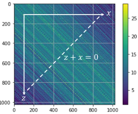
Figure 1.Gaussian test image generated artificially with a rapidly varying stochastic object field over thez-xpixel plane. Theyheight field is in arbitrary test units.
2.2. CARSCAN: Cartesian soil field extraction 193
To demonstrate the operation of these mathematical results over the DSM plane, we generate astochastic 194
object set (a tree field) over a Gaussian hill profile as shown in figure1and extract the soil and object
195
surfaces from it. The test field image is 1024×1024 and has a rapidly varying tree or object field over
196
the gaussian hill soil profile varying along the 45 degreez+x=0 diagonal (see figure1).
197
Repeatedly extracting a sections of the field along thezaxis generates an array ofyz(x)vectors alongx.
198
Each vector in this array can be operated on with Equation13to develop the soil profile at some value
199
ofzas a function ofx. Used in this way on the the entire profile array, equation13will generate asurface 200
soil field at some integration window widthw(see equation13). Here, instead of applying the spline
201
operatorSto the one dimensional Equation9, it is faster and more expedient from a computational
202
point of view to apply agridinterpolation operatorG(written in c++ and accessed via Python’s Numpy
203
framework for example) to the soil surface data,σ(x,z). Algorithm1codifies this methodology. 204
Algorithm 1Pseudocode description of a Cartesian soil field extraction
1: procedureCARSCAN(image,slices) 2: height←image height fromimage
3: width←image width fromimage
4: vertical scan at h: 5: fori∈ {0,height}do 6: raster scan at z=i:
7: forj∈ {0,width}do 8: raster=raster∪σ(i,j,w)
9: end for
10: rasterarr=rasterarr∪raster 11: end for
12: τ(i,j) =y(i,j)−G(rasterarr,y;i,j) 13: end procedure
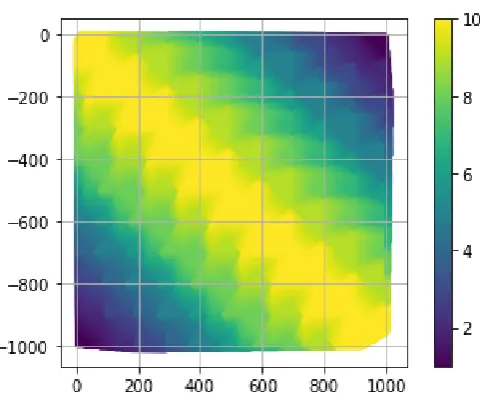
Theσ(x,z)field that results from algorithm1is shown in figure2. This functional representation of 205
the soil signal is then used to extract the object field variation over the terrain using Equation1directly,
206
resulting in the object fieldτ(x,z)which is shown in Figure3. 207
Due to the integral nature of the filter (equation13), algorithm1is quite noise resistant. It is also easy
208
to set for a variety of surfaces: for example,wcan be set manually or automatically to some fixed
209
percentage of the total number of points. It is usually a good idea to setwas large as the image size
210
will permit.
211
Figure 2.Soil fieldσ(x,z)extraction from the original Gaussian test field image.
τχ(x,z) = (
0, τ(x,z)≤ hτ(x,z)i
1, τ(x,z)>hτ(x,z)i (14)
allows a quick graphical appreciation of the object detection/classification area in the DSM model.
213
This is calculated in Figure4when the threshold level is set to the mean object field height.
214
2.3. FANSCAN: Moving radial soil field extraction 215
The integration method when generalised over many rasters line provides a convenient recipe for
216
separating the aerial image into object and soil fields as was shown in the Carscan algorithm above.
217
This Cartesian strategy can infact be envisaged alonganydirection in the image to yield information
218
particular to that orientation. The advantage of such rasterised vectoring (or radial scanning) of the
219
image is that it produces more information about the image frequencies in an off axis direction and is
220
therefore akin to a high resolution Fourier sampling of the ground object frequenciesωLalong some
221
lineL. The essential difference is that this is adirectand hence more stable methodology for sampling,
222
with the advantage that the numerical errors commonly associated with passages into and out of
223
transform spaces can be avoided while collecting information on those frequencies. An algorithm
224
designed around this principle would in theory be capable of obtaining the most complete directional
225
frequency scan of an image in direct space.
226
One method of achieving this is to make the series of direct horizontal rasters across the image in
227
the CARSCAN algorithm act as seeds for such a strategy. A given raster at(x=0,z)can be rotated
228
along any directionvin the image and rasterized to develop a one dimensional picture of the object
229
distributionalongthat line. Equation14would then develop the object and soil extractions for the
230
raster as planned earlier but in the directionv. Fanning the original raster(x = 0,z)along all the
231
possible directionsvforms a basis for theFANSCANalgorithm presented here (see algorithm2and
232
figure5).
233
FANSCAN delivers, therefore, the entire image surface as a series of raw data points classified along
234
their raster directions through the fan or direction vectorv(we take this symbol to mean both a
235
direction or discretization set of vectors as will be apparent from the context). Equation13applied
236
along any of these directions extracts the soil component of the raster and can be used to develop a
237
directionallysensitive picture of the soil structure at any point in the image. The data that contains this
238
information is a three dimensional point cloud which can be interpolated to fit the original point cloud
239
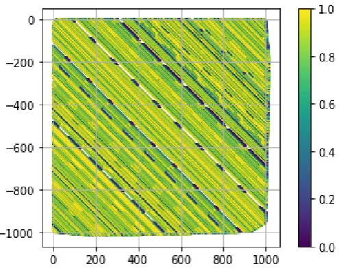
Figure 3.Object fieldτ(x,z)derived from equation3. Notice that the correlation frequency for these
objects is constant everywhere alongz+x=0.
Figure 4.The results of applying equation thresholding toτ(x,z)in figure3at the mean object field
height is the membership functionτχ(x,z). Notice that the correlation frequency for these objects is
constant everywhere alongz+x=0.
Algorithm 2Pseudocode description of FANSCAN
1: procedureFANSCAN(image,slices) 2: dθ←angular interval fromslices 3: h←image height fromimage
4: w←image width fromimage
5: vertical scan at h: 6: fori∈ {0,h}do
7: i0←i
8: raster scan atθ:
9: fork∈ {0,n−1}do
10: θ←the current raster angle fromk,dθ 11: L(θ,i0)←all points∈image on rasterθ
12: forx,y∈L(θ,i0)do
13: raster=raster∪image(x,y)
14: end for
15: end for
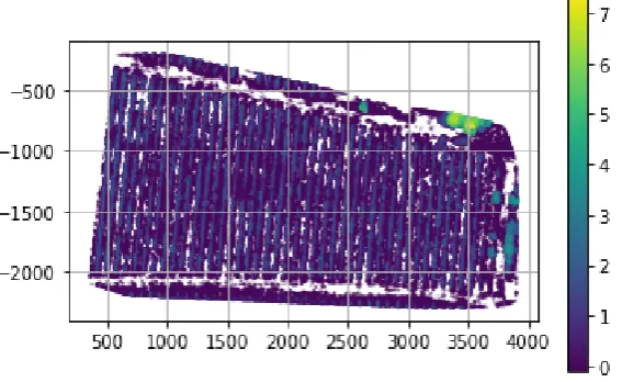
Figure 5.Geometry of the FANSCAN algorithm (see algorithm2). The white arrows are the raster vectorsvacross an extracted object field DSM. The dotted horizontal line is the current vertical scan position. Negative pixels on thezaxis are an artefact of matrix to image reflection. The vertical colorbar is in metres.
Once the DSM source σv(x,z)has been extracted from the FANSCAN algorithm in this way, the 241
original image and it can be subtracted over the plane to extract the three dimensional point cloud that
242
is in fact a high resolution object fieldτv(x,z)of the image in direct space. 243
In the context of this paper, we monitor the efficiency of the the algorithm as a function of the
244
discretization of the vector setsvto derive a relative extraction metric for the algorithm. Since the
245
theoretical benefit of using a radial scan in this manner is to provide more information on directional
246
object frequencies, such a metric can be naturally specified in terms of Fourier space frequencies
247
already introduced in equation6for the directionx.
248
Defining the Fourier space efficiency (or frequency reach) of a FANSCAN extractionηover some set of 249
discrete vectorsvas:
250
η(v,v∞) =1−kFFT∞−FFTvk2
kFFT∞k2 (15)
where FFT∞is the fast fourier transform of the original image and FFTvis the computed fast Fourier 251
transform ofσv(x,z) +τv(x,z), provides one such method for measuring the performance of the 252
extraction algorithm.
253
Equation15is a theoretical construct that is difficult to calculate since algorithm2extracts the object
254
field by computing the soil surface first. That is to say, the efficiency of the operation can only be
255
measured if the true soil surface were known, which it is not. However, there is a way around that
256
problem if we rewrite equation15as a sequencefor the extracted object field only:
257
η(vi,vi+1) =
kFFTvik2 kFFTvi+1k2
(16)
If the sequence of images generated by the FANSCAN algorithm is convergent in the space of images
258
(easy to prove) then:
259
lim
This relationship is dependent on the asymptotic convergence of the sequence of Fourier transforms
260
and is related to the convergence efficiencyη(v0,v∞)at the endpoints by:
261
η(v0,v∞) = ∞
∏
i=0η(vi,vi+1) (18)
A similar line of reasoning shows that the following general condition, where v0 is the simple 262
CARSCAN algorithm across the image, will be observed:
263
lim Nv→∞
∂η(v0,v)
∂Nv =0 (19)
where the algorithm has converged and byNvwe mean the resolution or number of vectors in setv.
264
It is therefore clear that∂η(v0,v)measures the quality of the processing operation between the initial 265
(CARSCAN) image result and the FANSCAN results wheni>0.
266
3. Results and Discussion 267
3.1. Data-set 268
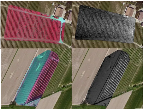
The study areas are located on a hilly farmland area. The acquisition campaigns were performed with
269
an AscTec Pelican equipped with the Sequoia multi-spectral camera. Figure6shows the study areas
270
and the related DSM. The final ortho products have a final Ground Sampling Distance (GSD) of 4
271
centimeters with 0.5 meters of horizontal accuracy.In both data-sets we planned to have a lateral and
272
longitudinal overlap above the 70%.
273
The quality of acquired data reflects on both orthophoto and DSM. Quality is mainly influenced by
274
the attitude of vehicle during the acquisition, height above the ground. This last aspect plays a key
275
role especially in hilly areas. If the mission was planned with a constant height each single image will
276
have a different GSD especially in areas with high slopes. We tried to set-up the acquisition by using a
277
constant height above the ground even if this required ana prioriknowledge of the DEM of area.
278
Study area 1 represents a hilly area of vineyards where several rows of trees are present also with
279
different displacement in the top area. Trees have an average height above the ground of 2 meters with
280
a small canopy at the top (0.7m).
281
Study area 2 represents an area covered by fruit plants with a small and constant slope over the area.
282
Trees have an average height above the ground of 2.5 metres with a large canopy at the top (up to 3m).
283
Figure 7.The first study area data set for testing the scanning algorithms; DSM Field at 2604×4381 pixels. The object field plantation ridges are barely visible to eye without segmentation. Equation14
can extract them efficiently nonetheless.
Figure 8.The second study area data set for testing the scanning algorithms; DSM at 4645×3465 pixels. This is a simple terrain map whose orientation exposes a flaw in the FANSCAN algorithm design.
3.2. FANSCAN vs CARSCAN 284
Using the same image DSM image as in Figure6and applying algorithm2obtains the interpolated
285
soil surfaceσv(x,z)as shown in figure11. The extracted object fieldτv(x,z)is given in figure12. The 286
extraction metric for this image can be seen in figure14.
287
To test and illustrate the method further we include a second DSM data-set seen in figure8.
288
Running FANSCAN on this data shows the theoretical consistency of the method and at the same time
289
an apparent weakness in its design.
290
When a raster vectorvfalls directly upon a row of trees, the soil extraction as developed in equation
291
13will fail. This aspect is nicely illustrated in figure17for the second dataset in figure8where part of
292
the object field gets extracted out with the soil field at aroundNv=100 fans.
Figure 9. The result of the FANSCAN soil extraction applied to figure7atNv =1 fan rasters per horizontal seed point. This corresponds to thev0CARSCAN algorithm in the example above. The
colour scale is in meters and negative pixel numbers are an artifact of the image to matrix conversion.
Figure 10.The result of the FANSCAN object extraction applied to figure7atNv=1 fan rasters per horizontal seed point. This corresponds to thev0CARSCAN algorithm in the example above. The
colour scale is in meters and negative pixel numbers are an artifact of the image to matrix conversion.
There are several solutions to this problem and all of them involve avoiding an encounter with such a
294
situation in the first place. The first possibility is to limit the maximum resolution (discretization of
295
the fanscan) manually. The second is to randomize both the horizontal seeding and the FANSCAN
296
rasterization. A combination of both of these measures can produce good results for the simple test
297
images as studied here but will fail in places for complex object field extractions.
298
The most costly, but a guaranteed solution, is to search successive soil field approximations for
299
competing minima and to reject any outliers from the soil field sequence. There are however
300
considerable difficulties in achieving this: the main one being that the physical number of points in
301
each extracted image is different and therefore extensive use of back interpolation needs to be made
302
to coregister the entire sequence being considered for correction. That can require lots of memory
303
(gigabytes) for even the most modest of images.
Figure 11.The result of the FANSCAN soil extraction applied to figure7atNv=100 fan rasters per horizontal seed point. The colour scale is in meters and negative pixel numbers are an artifact of the image to matrix conversion.
Figure 12.The result of the FANSCAN object extraction applied to figure7atNv=100 fan rasters per horizontal seed point. The colour scale is in meters and negative pixel numbers are an artifact of the image to matrix conversion.
While a fully automated solution can take time, in essence all that is actually required is one artifact
305
free image from the sequence so that artifacts in the sequence can be automaticallyrecognizedand then
306
removed. Following the discussion above, a good candidate for that image is the very first (CARSCAN)
307
iteration :v0. The logical matrix operation:
308
σv0i+1 = (σv0 ≥σvi+1)σvi+1+ (σv0 <σvi+1)σv0 (20) will quickly post process and correct the artifacts from the soil field. Figure21shows this correction
309
process applied to get back the corrected soil field for the FANSCAN atNv=100. The multiplicity
310
of rasters across the object field make it highly unlikely that the object field is adversely affected by
311
this phenomenon, so no correction need be applied. However, should one be necessary, it is easily
312
generated along with the soil field correction itself as shown in figure22.
Figure 13.The FANSCAN object characteristic applied to figure7atNv=100 fan rasters per horizontal seed point. The colour scale is in meters and negative pixel numbers are an artifact of the image to matrix conversion.
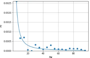
Figure 14.Equation19in practice for the DSM data of figure7: the closer the points are to the abscissa, the better the quality (convergence) of the image. The solid blue line is a power law nonlinear regression for the measured data and shows the likely value of the quality metric as a continuous function ofNv.
The theoretical basis of all these considerations is demonstrated by Equation19in the form of plots
314
of∂η shown for both data sets (see figures14,20). Moving backwards along the abcissa and hence 315
reducing the raster discretization to zero (that is towards the CARSCAN rasterization) shows an
316
accompanying depreciation in the Fourier space reach of the algorithm. In both cases the overall
317
accuracy evaluated over a ground truth as described in [28] is above the 95%.
318
4. Conclusions 319
In this paper we have presented two algorithms to segment crops and/or tree objects over soil by
320
using high-resolution images starting from Digital Surface Models that are usually available when the
321
data have been acquired by using unmanned platforms.
322
The approach is based on a two dimensional data slicing or reduction technique. Each slice is separately
323
processed as a one dimensional time series to derive the terrain and tree structures separately, here
324
interpreted as object probability densities. The results demonstrate that the method potentially enables
325
the correct segmentation of soil and can thus offer insights into the geometric distribution of surface
326
objects upon it.
327
A more sophisticated variant of this idea is the FANSCAN algorithm introduced above (see figure5 328
and algorithm2). It uses vector or radial raster scanning across the image to increase the frequency
329
resolution of the scanned data. The results are a generated sequence of images that converge onto the
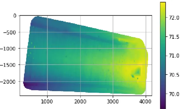
Figure 15.The result of the FANSCAN soil extraction applied to figure8atNv =1 fan rasters per horizontal seed point. This corresponds to thev0CARSCAN algorithm in the example above. The
colour scale is in meters and negative pixel numbers are an artifact of the image to matrix conversion.
Figure 16.The result of the FANSCAN object extraction applied to figure8atNv=1 fan rasters per horizontal seed point. This corresponds to thev0CARSCAN algorithm in the example above. The
colour scale is in meters and negative pixel numbers are an artifact of the image to matrix conversion.
original image. The frequency performance of the derived object field sequence was measured using a
331
Fourier efficiency metric which vanishes at infinite time.
332
Due to real world considerations it would be prudent to ally the quality metric with a measure of the
333
number of processor cycles at timetto define an overall functional of performance. The unique limit
334
point of the image sequence in direct and Fourier spaces means that such a functional would be a
335
global optimizer for the algorithm.
336
An apparent drawback of the FANSCAN algorithm is that it will run into trouble when it encounters
337
a coincident object field line (such as an avenue of trees) as has been seen in figure17. If a raster
338
line lies on top of one of these arrays then the soil extractor will suddenly reduce its efficiency and
339
real objects will tend to creep into the soil field. A costly, but accurate method for dealing with these
340
situations is to post process the image against a lower resolution image soil field construction where
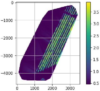
Figure 17. The result of the FANSCAN soil extraction applied to figure8atNv =100 fan rasters per horizontal seed point. Note how certain parts of the object field have been included in the soil extraction. The colour scale is in meters and negative pixel numbers are an artifact of the image to matrix conversion.
Figure 18.The result of the FANSCAN object extraction applied to figure8atNv=100 fan rasters per horizontal seed point. The colour scale is in meters and negative pixel numbers are an artifact of the image to matrix conversion.
raster discretization avoids this situation. Cross elimination of coincident maxima then removes the
342
artifacts and both the object and soil fields can thus be corrected at higher resolution scans. Equation
343
20is an example of one such measure. Of course, a fairly convergentlow resolutionFANSCAN lowers
344
the probability of this occurring. An added bonus is that the same strategy lowers the runtime for the
345
algorithm. For these reasons, a high resolution FANSCAN is not in general recommended.
346
For upcoming research we will perform more tests also evaluating a pure random approach in terms
347
of radial direction and radial ray’s start that tries to mix the advantages of CARSCAN and FANSCAN.
348
Acknowledgments:The authors would like to thank Carlo Alberto Bozzi of EVE S.r.l. for his valuable support 349
Figure 19.The FANSCAN object characteristic applied to figure8atNv=100 fan rasters per horizontal seed point. The colour scale is in meters and negative pixel numbers are an artifact of the image to matrix conversion.
Figure 20.Equation19in practice for the DSM data of figure8: the closer the points are to the abcissa, the better the quality (convergence) of the image. The solid blue line is a power law nonlinear regression for the measured data and shows the likely value of the quality metric as a continuous function ofNv.
Author Contributions:Professors Frontoni and Zingaretti are responsible for carrying out research on the various 351
segmentation approaches referred to in this article. Prof. Adriano Mancini and Dr Jack Dyson have worked on the 352
rasterization analysis and extraction techniques for theσandτdigital vector fields used in this work.
353
354
1. Colomina, I.; Molina, P. Unmanned aerial systems for photogrammetry and remote sensing: A review. 355
{ISPRS} Journal of Photogrammetry and Remote Sensing2014,92, 79 – 97. 356
2. Enciso, J.; Maeda, M.; Landivar, J.; Avila, C.; Jung, J.; Chang, A. Unmanned aerial system (UAS) for 357
precision agriculture and management decisions. 2016. 358
3. Candiago, S.; Remondino, F.; De Giglio, M.; Dubbini, M.; Gattelli, M. Evaluating Multispectral Images and 359
Vegetation Indices for Precision Farming Applications from UAV Images.Remote Sensing2015,7, 4026. 360
4. Matese, A.; Toscano, P.; Di Gennaro, S.F.; Genesio, L.; Vaccari, F.P.; Primicerio, J.; Belli, C.; Zaldei, A.; 361
Bianconi, R.; Gioli, B. Intercomparison of UAV, Aircraft and Satellite Remote Sensing Platforms for Precision 362
Viticulture.Remote Sensing2015,7, 2971–2990. 363
5. Bernardini, A.; Frontoni, E.; Malinverni, E.; Mancini, A.; Tassetti, A.; Zingaretti, P. Pixel, object and hybrid 364
classification comparisons.Journal of Spatial Science2010,55, 43–54. 365
6. Hedley, C. The role of precision agriculture for improved nutrient management on farms. Journal of the 366
Figure 21.The result of the FANSCAN soil field correction applied to figure17atNv=100 fan rasters per horizontal seed point. The correction eliminates the parts of the object field included into the image from figure18. The colour scale is in meters and negative pixel numbers are an artifact of the image to matrix conversion.
Figure 22. The result of the FANSCAN object field correction applied to figure8atNv =100 fan rasters per horizontal seed point. The correction adds the parts of the object field included into the image from figure18. The colour scale is in meters and negative pixel numbers are an artifact of the image to matrix conversion.
7. Schenatto, K.; de Souza, E.; Bazzi, C.; Gavioli, A.; Betzek, N.; Beneduzzi, H. Normalization of data for 368
delineating management zones.Computers and Electronics in Agriculture2017,143, 238–248. 369
8. Jin, Z.; Prasad, R.; Shriver, J.; Zhuang, Q. Crop model- and satellite imagery-based recommendation tool 370
for variable rate N fertilizer application for the US Corn system. Precision Agriculture2017,18, 779–800. 371
9. De Benedetto, D.; Castrignanò, A.; Rinaldi, M.; Ruggieri, S.; Santoro, F.; Figorito, B.; Gualano, S.; Diacono, 372
M.; Tamborrino, R. An approach for delineating homogeneous zones by using multi-sensor data. Geoderma 373
10. Yang, C.; Odvody, G.; Fernandez, C.; Landivar, J.; Minzenmayer, R.; Nichols, R. Evaluating unsupervised 375
and supervised image classification methods for mapping cotton root rot. Precision Agriculture2015, 376
16, 201–215. 377
11. Zurita-Milla, R.; Izquierdo-Verdiguier, E.; De By, R. Identifying crops in smallholder farms using time 378
series of WorldView-2 images. 2017. 379
12. Varela, S.; Assefa, Y.; Vara Prasad, P.; Peralta, N.; Griffin, T.; Sharda, A.; Ferguson, A.; Ciampitti, I. 380
Spatio-temporal evaluation of plant height in corn via unmanned aerial systems.Journal of Applied Remote 381
Sensing2017,11. 382
13. Iqbal, F.; Lucieer, A.; Barry, K.; Wells, R. Poppy crop height and capsule volume estimation from a single 383
UAS flight. Remote Sensing2017,9. 384
14. Erten, E.; Lopez-Sanchez, J.; Yuzugullu, O.; Hajnsek, I. Retrieval of agricultural crop height from space: A 385
comparison of SARtechniques.Remote Sensing of Environment2016,187, 130–144. 386
15. Aasen, H.; Burkart, A.; Bolten, A.; Bareth, G. Generating 3D hyperspectral information with lightweight 387
UAV snapshot cameras for vegetation monitoring: From camera calibration to quality assurance. ISPRS 388
Journal of Photogrammetry and Remote Sensing2015,108, 245–259. 389
16. De Souza, C.; Lamparelli, R.; Rocha, J.; Magalhães, P. Height estimation of sugarcane using an unmanned 390
aerial system (UAS) based on structure from motion (SfM) point clouds. International Journal of Remote 391
Sensing2017,38, 2218–2230. 392
17. Chaves, A.; La Scalea, R.; Colturato, A.; Kawabata, C.; Furtado, E.; Branco, K. Using UAVs and digital 393
image processing to quantify areas of soil and vegetation. Journal of Physics: Conference Series2015,633. 394
18. Yue, J.; Yang, G.; Li, C.; Li, Z.; Wang, Y.; Feng, H.; Xu, B. Estimation of winter wheat above-ground biomass 395
using unmanned aerial vehicle-based snapshot hyperspectral sensor and crop height improved models. 396
Remote Sensing2017,9. 397
19. Malambo, L.; Popescu, S.; Murray, S.; Putman, E.; Pugh, N.; Horne, D.; Richardson, G.; Sheridan, R.; Rooney, 398
W.; Avant, R.; Vidrine, M.; McCutchen, B.; Baltensperger, D.; Bishop, M. Multitemporal field-based plant 399
height estimation using 3D point clouds generated from small unmanned aerial systems high-resolution 400
imagery. International Journal of Applied Earth Observation and Geoinformation2018,64, 31–42. 401
20. Torres-Sanchez, J.; Lopez-Granados, F.; Serrano, N.; Arquero, O.; Pena, J. High-throughput 3-D monitoring 402
of agricultural-tree plantations with Unmanned Aerial Vehicle (UAV) technology. PLoS ONE2015,10. 403
cited By 20. 404
21. Lopez-Granados, F.; Torres-Sanchez, J.; De Castro, A.I.; Serrano-Perez, A.; Mesas-Carrascosa, F.J.; Pena, 405
J.M. Object-based early monitoring of a grass weed in a grass crop using high resolution UAV imagery. 406
Agronomy for Sustainable Development2016,36. 407
22. Perez-Ortiz, M.; Pena, J.; Gutierrez, P.; Torres-Sanchez, J.; Hervas-Martinez, C.; Lopez-Granados, F. 408
Selecting patterns and features for between- and within- crop-row weed mapping using UAV-imagery. 409
Expert Systems with Applications2016,47, 85–94. 410
23. Perez-Ortiz, M.; Pena, J.; Gutierrez, P.; Torres-Sanchez, J.; Hervas-Martinez, C.; Lopez-Granados, F. A 411
semi-supervised system for weed mapping in sunflower crops using unmanned aerial vehicles and a crop 412
row detection method.Applied Soft Computing Journal2015,37, 533–544. 413
24. Hamuda, E.; Mc Ginley, B.; Glavin, M.; Jones, E. Automatic crop detection under field conditions using the 414
HSV colour space and morphological operations.Computers and Electronics in Agriculture2017,133, 97–107. 415
25. Kiani, S.; Jafari, A. Crop Detection and Positioning in the Field Using Discriminant Analysis and Neural 416
Networks Based on Shape Features. Journal of Agricultural Science and Technology2012,14, 755–765. 417
26. Delenne, C.; Rabatel, G.; Deshayes, M. An Automatized Frequency Analysis for Vine Plot Detection and 418
Delineation in Remote Sensing. IEEE Geoscience and Remote Sensing Letters2008,5, 341–345. 419
27. Comba, L.; Gay, P.; Primicerio, J.; Ricauda Aimonino, D. Vineyard detection from unmanned aerial systems 420
images. Computers and Electronics in Agriculture2015,114, 78–87. 421
28. Mancini, A.; Dyson, J.; Frontoni, E.; Zingaretti, P. Soil / crop segmentation from remotely sensed data 422
acquired by Unmanned Aerial System. 2017 International Conference on Unmanned Aircraft Systems 423
(ICUAS), 2017, pp. 1410–1417. 424
29. Khoshelham, K.; Nardinocchi, C.; Frontoni, E.; Mancini, A.; Zingaretti, P. Performance evaluation of 425
automated approaches to building detection in multi-source aerial data.ISPRS Journal of Photogrammetry 426
30. Mancini, A.; Frontoni, E.; Zingaretti, P. AUTOMATIC EXTRACTION OF URBAN OBJECTS FROM 428
MULTI-SOURCE AERIAL DATA.ISPRS - International Archives of the Photogrammetry, Remote Sensing and 429
Spatial Information Sciences2009,XXXVIII-3/W4, 13–18. 430
31. Mancini, A.; Frontoni, E.; Zingaretti, P.; Longhi, S. High-resolution mapping of river and estuary areas by 431
using unmanned aerial and surface platforms. 2015 International Conference on Unmanned Aircraft Systems, 432