Horizontal Diffraction in Multiple Obstacles Using Parabolic
Equation with Recursive Convolution Nonlocal Boundary Conditions
Zan-Yu Ge, Gui-Zhen Lu*, Huai-Bao Xiao, Dong-Dong Zeng, and Abomakhleb Gheit
Abstract—The accuracy of wave propagation prediction is very important in telecommunication network planning. The parabolic equation model has an advantage in computation efficiency and accuracy for wave propagation prediction. The recursive convolution nonlocal boundary condition has an advantage in improving the computational efficiency. In this paper, the recursive convolution nonlocal boundary conditions are extended to deal with the issue of horizontal diffraction loss in multiple obstacles. The validation is performed with experiments and the results show a good agreement.
1. INTRODUCTION
Parabolic Equation Model (PEM) is derived from the Helmholtz equation which ignores the influence of the back-scattering or spread of the waves and only has the forward propagation approximation, then the second order elliptic equations are simplified into first order parabolic equation on direction of propagation [1, 2]. This model can facilitate a marching-in range technique for numerical computation. It can also deal with the horizontal and vertical directions of the environment where mediums are uneven distribution. Therefore, PEM as a deterministic model has been widely used in wireless communications, broadcasting, optics, radar and computational electromagnetics communities in various electrically-large electromagnetic applications such as radio wave propagation modelling over irregular terrains [3], radar cross-section simulations [4], and x-band applications [5]. There are two schemes available for the solution of PE, the first of which is the split-step Fourier transform (SSFT) method [6] that is applicable when analytical eigenfunction exists for the underlying geometry. Although this technique is numerically very fast and efficient in large dimensions wave propagation problems, it is inconvenient for irregular terrain boundary modeling. The other scheme is the finite difference (FD) method [7, 8] which is applicable to more general geometries with boundaries. And using FD on parabolic equation can simplify matrix transformation form of space field, and almost any near-field region can be obtained by a field on the surface of the former through a simple matrix transformation. The subject matter of this paper is applicable to the latter.
At present, most of the research about obstacles diffraction loss mainly focuses on the three-dimensional PEM [9] and the vertical diffraction of two-three-dimensional PEM [10, 11]. But in some cases, radio wave is spread mainly through horizontal diffraction instead of vertical diffraction if the obstacle’s height is much larger than the width. In order to solve this problem, a 2D FD-PEM is used to calculate the propagation loss of the multiple obstacles horizontal diffraction.
For simulating the radio wave propagation spread in infinite space, the boundary conditions (BC) must be specified at both sides of the computational domain and inserted into the FD-PEM code. For the PEM, there are several boundary conditions to truncate the infinite space, such as the perfectly matched layer (PML) BC [12], absorbing layer BC [13] and nonlocal boundary condition (NLBC) [14, 15]. The first two BCs are computationally expensive, because they increase considerably the size of the
Received 15 March 2017, Accepted 27 April 2017, Scheduled 9 May 2017 * Corresponding author: Gui-Zhen Lu ([email protected]).
computational domain and often introduce parasitic reflections at the same time. The NLBC is an exact BC that does not require additional computation space. And it takes into account the global nature of the solution and not just its local properties. Furthermore, using NLBC does not oppose the marching character of PE solutions because only previous ranges are involved. However, NLBC also has a disadvantage: computations time-consuming for spatial convolution integral. This computation is also memory demanding as it requires the storage and use of all previous values of the field along the boundary. In view of these problems, recursive convolution (RC) with vector fitting is proposed by Mias in [16] to approximate the convolution integral terms, which can eliminate these disadvantages. The method is used to model wave propagation in the infinite space without the obstacles
So far, there are no researchers using the recursive convolution nonlocal boundary conditions (RC-NLBC) to calculate the diffraction loss in multiple obstacles. Here, the method is used to study the wave propagation in the complex environment with multiple obstacles. Considering the horizontal diffraction has significant effects in some cases, the PEM with RC-NLBC is used for the horizontal diffraction problem. The boundary condition is modified to suit the horizontal diffraction. Thus, this BC was used on the left boundary and the right boundary in 2D finite difference parabolic equation model (FD-PEM) to predict the propagation loss of horizontal diffraction. In order to validate the computed results, the laboratory experiment is performed for wave propagation in the multiple obstacles environment. Finally, the calculated results are compared with the measured data from experimental platform.
2. FINITE DIFFERENCE PARABOLIC EQUATION METHOD
Considering the horizontal diffraction problem, the wave equation in free space [1] is defined as:
∂2ψ(x, y)
∂x2 +
∂2ψ(x, y)
∂y2 +k
2n2ψ(x, y) = 0. (1)
where ψ(x, z) is the field variable, ψ = Ey for TE polarization and ψ = Hy for TM polarization.
k = 2π/λ is the wavenumber, λ the wavelength and n the refractive index. The positive direction of theX axis is the direction of propagation as shown in Fig. 1, and the width of propagation domain is represented asy.
X
Figure 1. Sketch map of propagation.
If we define field variable as
ψ(x, y) =e−jkxu(x, y) (2) Then substituting Eq. (2) in Eq. (1)
∂2u ∂x2 −2jk
∂u ∂x+
∂2u ∂y2 +k
2(n2−1)u= 0 (3)
Equation (3) can be decomposed for
[
∂ ∂x+jk
(√
Q−1
)] [ ∂
∂x−jk
(√
Q+ 1
)]
The differential operatorQ is represented as
Q=1
k2
∂2 ∂y2 +n
2 (5)
Ignoring the backward wave, we can get the forward wave equation in the form of parabola:
∂u
∂x =−jk
(√
Q−1
)
u (6)
Using the Pade approximation [1, 17]
√ Q= 1+3 4 ( 1 k2 ∂2 ∂y2 +n
2−1
) 1+1 4 ( 1 k2 ∂2 ∂y2 +n
2−1
) (7)
Substituting Eq. (7) in Eq. (6)
∂2u(x, y)
∂y2 −j2k
∂u(x, y)
∂x − j
2k
∂3u(x, y)
∂y2∂x = 0 (8)
The central finite difference approximation is given by [1, 16]
u
[(
m−1
2
)
∆x, n∆y
]
= f m
n +fnm−1
∆x ;
∂u
[(
m−1
2
)
∆x, n∆y
]
∂x =
fnm−fnm−1
∆x ;
∂2u[m∆x, n∆y]
∂y2 =
fnm−1−2fnm+fnm+1
(∆y)2
(9)
Combining Eq. (9) with Eq. (8), the finite difference parabolic equation is obtained as following
αmumn−1+βmumn +αmumn+1 =αm−1umn−−11+βm−1umn−1+αm−1umn+1−1 (10) where
αm−1 = 1 4k2∆y2 −
j∆x
4k∆y2, αm= 1 4k2∆y2 +
j∆x
4k∆y2;
βm−1 = 1 +
j∆x
2k∆y2 − 1
2k2∆y2, βm= 1−
j∆x
2k∆y2 − 1 2k2∆y2.
3. RECURSIVE CONVOLUTION NONLOCAL BOUNDARY CONDITIONS AND ITS FINITE DIFFERENCE SCHEME
Nonlocal boundary condition is presented in [14] as shown below:
∂u(x, y)
∂y =yinc(x)−jτ2k
∫ x
0
w(x−ξ)∂u(ξ, y)
∂ξ dξ (11)
where
yinc(x) =
∂uinc(x, y)
∂y +jτ2k
∫ x
0
w(x−ξ)∂uinc(ξ, y)
∂ξ dξ (12)
Mias implements recursive convolution to convolution integral terms and vector fitting to Bessel function for Equation (11) in [16]. So the RC-NLBC expressions that discretized by second order accurate discretization is represented as
umA =µumB +ωumC + Γm,A (14) where at the right boundary A = 0, B = 1, C = 2 and at the left boundary A = N, B = N −1 and C =N−2. N is the number of discrete points on theY axis. In addition,
µ = 4
3+2ζ∆y; ω=−
−1 3+2ζ∆y;
ΓmA = uinc,mA −µuinc,mB −ωuinc,mC + µζ∆y 2
(
umA−1−uinc,mA −1
)
−µ∆y 2
(
Φum,A−Φincm,A);
Φm,A = 2jk 20
∑
i=1
ek(bi−j)∆xRm−1
i ;
Rmi = ek(bi−j)∆xRm−1
i +ai (
1−ek(bi−j)∆x
−k(bi−j) ∆x )
(
umA−umA−1);
ζ = 2jk
20
∑
i=1
ai (
1−ek(bi−j)∆x
−k(bi−j) ∆x )
The values ofai andbi can refer to literature [16]. Substituting Eq. (14) in Eq. (10), the matrix equation to solve the problem of Fig. 1 is shown below
AmUm = Am−1Um−1+ B, (15)
where
Um =
um1 um2 um3
.. .
umN−3 umN−2 umN−1
; Um−1 =
um1−1 um2−1 um3−1
.. .
umN−−13 umN−−12 umN−−11
; B =
αm−1um0 −1 0 0 .. . 0 0
αm−1umN−1 −
αmΓm,0 0 0 .. . 0 0
αmΓm,N ;
Am =
βm′ αm′ 0 · · · 0 0 0
αm βm αm · · · 0 0 0 0 αm βm · · · 0 0 0
..
. ... ... ... ... ... ... 0 0 0 · · · βm αm 0 0 0 0 · · · αm βm αm 0 0 0 · · · 0 α′m βm′
;
Am−1 =
βm−1 αm−1 0 · · · 0 0 0
αm−1 βm−1 αm−1 · · · 0 0 0 0 αm−1 βm−1 · · · 0 0 0
..
. ... ... ... ... ... ...
0 0 0 · · · βm−1 αm−1 0 0 0 0 · · · αm−1 βm−1 αm−1 0 0 0 · · · 0 αm−1 βm−1
;
βm′ = βm+µαm;α
′
4. EXPERIMENT SETUP
As illustrated in Fig. 2(a), the measurements are made by transmitting a continuous wave signal which were generated by the Agilent Signal Generator. The transmitter output power was 15 dBm. The transmitting antenna for the measurements was a quarter wavelength monopole antenna, and the gain of it was ignored. The Agilent Spectrum Analyzer was used as a receiver with very narrow bandwidth. The receiving antenna was a waveguide antenna, having a gain of 0 dBi and working at the frequencies from 8 GHz to 10 GHz. According to the aforementioned properties of experiment equipment, the working frequency was chosen at 9.375 GHz. The experiment environment is shown in Fig. 2(b). Both the transmitting antenna and receiving antenna are set on an aluminous plane which was surrounded by wave-absorbing materials to simulate free space propagation environment. Their height can be ignored. The maximum distance between the two antennas is 2.3 m. According to Huygens-Fresnel principle, the maximum radius of first Fresnel zone is 13.56 cm. The obstacles are all bricks surrounded by copper foil, and their height, width, thickness are 23 cm, 7.5 cm and 3 cm, respectively. The height of obstacle in vertical is far larger than the maximum radius of the first Fresnel zone, and in horizontal one the obstacle width is less than the maximum radius of the first Fresnel zone. Thus the influence of vertical diffraction can be ignored.
For the incoherent scattering from surrounding absorbing materials, due to the lower reflection coefficient of absorbing materials, the propagation path of scattering wave is at least two times larger than directed wave path from the transmitter to receiver, and the incoherent wave is ignored in the experiment.
The influence of atmospheric medium for wave propagation can be ignored in an ideal atmospheric
(a) (b)
Figure 2. Measurement system and experiment environment setup. (a) Measurement system setup, (b) experiment environment setup.
environment. The free space propagation loss is given by [18]
L= 32.45 + 20 lgf(MHz)+ 20 lgr(km) (16)
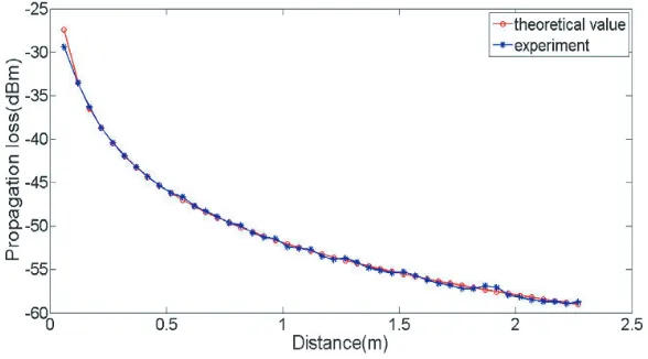
In order to verify the accuracy of the experimental platform, field distribution was measured in free space. Namely, when there is no obstacle on the propagation path, move the position of the Rx antenna. And the average results of several experiments were compared with the theoretical value, as shown in Fig. 3.
According to Fig. 3, the theoretical values agree well with the experimental data, which proves the reliability of experimental platform.
5. MEASUREMENTS AND RC-NLBC-FD-PEM COMPUTING
In order to fit the experimental requirements, a special case of the tapered wave [19, 20] is applied to RC-NLBC-FD-PEM code as the incident field.
f(0, y) = √ 1 P√π/2
exp [(−jk·sinθ)·y] exp
[
−
(
y−b
P
)2]
(17)
where
P = √
2 log 2
k·sin (φ/2)
θis the elevation angle of the beam,φthe beam width andbthe distance between antenna and original location.
The simulation parameters in RC-NLBC-FD-PEM are θ= 0, φ=π/36, λ= 0.032 m, b= 0.6 m, ∆x= 0.01 m, ∆y= 0.01 m, y= 1 m (refer to Fig. 1 and Eq. (17)).
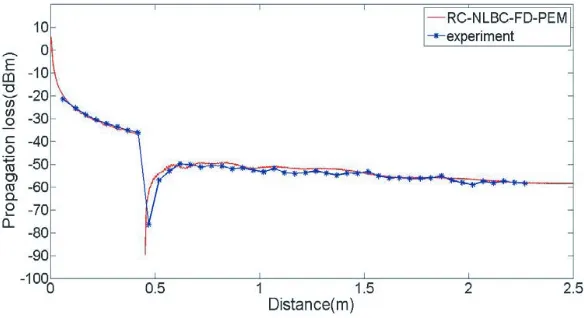
5.1. Horizontal Diffraction Cases of Single Obstacle
As shown in Fig. 1, obstacle is placed on the propagation path. The distance from obstacle to transmitter is 42 cm, and comparison of measured dates and calculation results are shown in Fig. 4.
Figure 4. Comparison of measured dates and calculation results in case of single obstacle (refer to Fig. 1).
5.2. Horizontal Diffraction Cases of Double Obstacles
(a)
(b)
Figure 5. Double obstacles. (a) Location of the double obstacles, (b) comparison of measured dates and calculation results.
(a) (b)
Figure 6. Location of obstacles.
(a) (b)
Figure 7. Comparison of measured dates and calculation results. (a) d0 = 60 cm, d1 = d2 = 3.2 cm,
5.3. Other Horizontal Diffraction Cases
The comparison results are given by Fig. 7 in other cases, and the obstacles locations are shown in Fig. 6.
6. CONCLUSION
In order to deal with the issue of the horizontal diffraction of the radio wave propagation, recursive convolution nonlocal boundary condition was used for finite difference parabolic equation model to calculate the diffraction loss in multiple obstacles. An indoor radio wave propagation loss measurement environment which worked at 9.375 GHz was built, and a series of experiments were implemented. Because the experiment may have reflection and interference phenomenon, measurements may cause slight fluctuation. The comparison results in Figs. 4, 5, 7 confirm that the trend of RC-NLBC-FD-PEM and experiment are basically identical. Therefore, RC-NLBC-FD-RC-NLBC-FD-PEM can be used to predict horizontal diffraction propagation loss effectively. In this paper, the RC-NLBC is extended to deal with the issue of horizontal diffraction loss at multiple obstacles environment, and the effectiveness of the approach is verified by experiments. The application of RC-NLBC in PEM provides a new research idea and method for the wave propagation prediction. For now, RC-NLBC has only been applied to the two-dimensional PEM, and subsequent work will be extended to three dimensional spaces.
REFERENCES
1. Levy, M. F., Parabolic Equation Methods for Electromagnetic Wave Propagation, IEE Press, London, 2000.
2. Donohue, D. J. and J. R. Kuttler, “Propagation model in over terrain using the parabolic wave equation,”IEEE Transactions on Antennas and Propagation, Vol. 48, No. 1, 824–827, 2001. 3. Wang, K. and Y. L. Long, “Propagation modeling over irregular terrain by the improved two-way
parabolic equation method,” IEEE Transactions on Antennas and Propagation, Vol. 60, No. 9, 4467–4471, 2012.
4. Huang, Z. X., Q. Wu, and X. L. Wu, “Solving multi-object radar cross section based on wide-angle parabolic equation method,”Systems Engineering and Electronics, Vol. 17, No. 4, 722–724, 2006. 5. Chiou, M. M. and J. F. Kiang, “Simulation of X-band signals in a sand and dust storm with
parabolic wave equation method and two-ray model,” IEEE Antennas and Wireless Propagation Letters, No. 99, 2016.
6. Valtr, P., P. Pechac, V. Kvicera, and M. Grabner, “A radiowave propagation study in an urban environment using the fourier split-step parabolic equation,”The Second European Conference on Antennas and Propagation, EuCAP 2007, 2007.
7. Aklilu, T. and G. Giorges, “Finite element and finite difference methods for elliptic and parabolic differential equations,” Numerical Analysis — Theory and Application, Prof. Jan Awrejcewicz (Ed.), InTech, 2011, ISBN: 978-953-307-389-7.
8. Fadugba, S. E., O. H. Edogbanya, and S. C. Zelibe, “Crank Nicolson Method for solving parabolic partial differential equations,” IJA2M, Vol. 1, No. 3, 8–23, 2013.
9. Silva, M. A. N., E. Costa, and M. Liniger, “Analysis of the effects of irregular terrain on radio wave propagation based on a three-dimensional parabolic equation,” IEEE Transactions on Antennas and Propagation, Vol. 60, No. 4, 2138–2143, 2012.
10. Sevgi, L., C. Uluisik, and F. Akleman, “A MATLAB-based two-dimensional parabolic equation radiowave propagation package,” IEEE Antennas and Propagation Magazine, Vol. 47, No. 4, 164– 175, 2005.
11. Bai, R. J., C. Liao, N. Sheng, and Q. H. Zhang, “Prediction of wave propagation over digital terrain by parabolic equation model,”IEEE International Symposium on MAPE, Oct. 29–31, 2013. 12. Keefe, K., “Dispersive waves and PML performance for large-stencil differencing in the parabolic
13. Zhang, P., L. Bai, Z. Wu, and F. Li, “Effect of window function on absorbing layers top boundary in parabolic equation,”Antennas and Propagation (APCAP), Jul. 26–29, 2014.
14. Dalrymple, R. A. and P. A. Martin, “Perfect boundary conditions for parabolic water-wave models,”
Proc. R. Soc. London A, Vol. 437, 41–54, 1992.
15. Zebic-Le Hyaric, A., “Wide-angle nonlocal boundary conditions for the parabolic wave equation,”
IEEE Transactions on Antennas and Propagation, Vol. 49, No. 6, 916–922, 2001.
16. Mias, C., “Fast computation of the nonlocal boundary condition in finite difference parabolic equation radiowave propagation simulations,” IEEE Transactions on Antennas and Propagation, Vol. 56, No. 6, 1699–1705, 2008.
17. Claerbout, J. F., Fundamentals of Geophysical Data Processing with Application to Petroleum Prospect, McGraw-Hill Press, New York, 1976.
18. Mardeni, R. and K. F. Kwan, “Optimization of hata propagation prediction model in suburban area in Malaysia,”Progress In Electromagnetics Research C, Vol. 13, 91–106, 2010.
19. Chang, W. and L. Tsang, “A partial coherent physical model of third and fourth Stokes parameters of Sastrugi snow surfaces over layered media with rough surface boundary conditions of conical scattering combined with vector radiative transfer theory,” Progress In Electromagnetics Research B, Vol. 45, 57–82, 2012.