Thinning a Subset of Selected Elements for Null Steering Using
Binary Genetic Algorithm
Jafar R. Mohammed*
Abstract—Generally, the null steering is performed by controlling the amplitude and/or phase weightings of all element excitations or only a small number of them. In such cases, a need for extra RF components such as variable attenuators and variable phase shifters with each element in the array is inevitable. In this paper, an alternative method is introduced where the null steering is performed by thinning (or turning off) only a small subset of the elements in the uniform linear arrays. To find an optimum combination of active (on) and inactive (off) elements, a binary genetic algorithm is used. In large arrays, the number of required nulls is much smaller than the total number of array elements, thus only a small subset of the array elements could be sufficient for producing the required nulls rather than optimizing all the array elements. By this way, a faster convergence speed of the optimizer and lowest peak sidelobe level can be obtained. The effectiveness of the proposed method with various subset configurations will be demonstrated and compared with some standard null steering methods.
1. INTRODUCTION
Adaptive nulling is one of the important and essential functions of the smart antenna in the fifth generation (5G) wireless communication systems to effectively suppress the interfering signals and efficiently improves the output signal to interference plus noise ratio (SINR). Generally, null steering has been performed by controlling the amplitude weighting [1] and/or phase weighting [2] of all element excitations or only a small subset of them [3–5] or even only two edge elements [6, 7]. Although these methods guarantee effective cancelation of the interfering signals, an increase in the antenna array structures and feeding networks with respect to that of the uniformly excited arrays is unavoidable. To keep the antenna structure and feeding network as simple as possible, thinning techniques have been proposed in the literature [8, 9]. In such thinned arrays, a number of active elements that have uniform amplitude excitations are connected to the feeding network, while those inactive elements which have zero amplitude excitations are connected to the matched loads.
Clearly, with the thinned arrays neither attenuators nor phase shifters are required. Also, the number of the active elements is greatly reduced while providing better radiation characteristics such as low sidelobe level. Thus, the thinned arrays have been widely used in the satellite communications [10] and radar systems [11]. In these applications, the main goals of the thinning were to minimize the number of active elements and the sidelobe levels in the resulting thinned array pattern while still providing nearly the same narrow beamwidth as that of the uniformly array pattern (fully filled array) under the condition of same array length.
Designing the thinned arrays with analytical procedures is not possible due to the unavailability of the closed-form solutions. Thus, they are mostly designed in the literature by using global evolutionary optimization algorithms such as genetic algorithms (GA) [12, 13], particle swarm optimizer (PSO) [14, 15], and ant colony optimizer (ACO) [16] where they proved to be powerful tools for efficiently
Received 16 February 2018, Accepted 30 March 2018, Scheduled 13 April 2018
* Corresponding author: Jafar Ramadhan Mohammed ([email protected]).
optimizer to reach the optimum ones that meet the desired goals. Also, with such a huge number of the examination trials (combinations) especially when dealing with large arrays a very slow convergence speed is a real challenging issue. This problem has been clearly identified in the literature for example see [17, 18] and, thus, hybrid methods [19–22] have been proposed to address such problem.
In this paper, the thinning process is performed only on a small subset of array elements to achieve the required nulls. Unlike the concept of sidelobe level minimization, the null steering can be performed with only a subset of array elements because the required number of the nulls is much smaller than the total number of the array elements. Thus, null steering could be accomplished by thinning only a small subset of array elements instead of all the array elements while providing the same capability for interference suppression. By this manner, not only the required nulls can be achieved, but also a significant improvement on the convergence speed of the optimizer can be obtained. Various configurations may exist for selecting such subset array elements. The subset array could be selected from center or outer elements of the array or any other configuration including random selection. It is shown well that the most appropriate configurations is the outer one whose elements are selected from extreme elements of the array. This is mainly because extreme elements have a great influence on the generated nulls [23]. Regarding this important fact, it is worthy to mention that the authors in [23, 24] achieved the desired pattern by changing the positions of the zeros of the array factor and placing them closer together in the suppression region and further apart elsewhere. By this way, they noted that such suppression required modification of the aperture distribution was only near the ends of the array [24]. This observation is exploited in this paper to select a proper subset configuration. Simulation results will be given for 100-element linear arrays of various subset configurations to confirm the most appropriate configuration that provides the required single, multiple and wide nulls. Moreover, the null steering performance of the selected configurations is tested under various degrees of thinning, ranging from highly filled to massively thinned.
2. THE STANDARD NULL STEERING METHOD
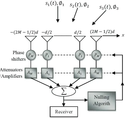
Figure 1 shows a general block diagram of the standard null steering method that consists of a main control called nulling algorithm and two separate sets of variable attenuators and phase shifters for weighting the amplitude and phase excitations of each element in the array. Assume that the array is symmetric about the center of the array and has an even number of elements N = 2M. In such a case, the numbers of variable attenuators and phase shifters are reduced to half. In the standard null steering scenario, we also assume that a number of signals equal toI are arriving from directions∅i with voltage
si(t), then the array factor can be given by
AF(ui) =w∗me−j( 2M−1
2 )kdui+. . .+w1∗e−j(
1
2)kdui+w1ej(
1
2)kdui+. . .+wmej( 2M−1
2 )kdui (1)
and the normalized overall array output is
Array Output = 1
m
wm I
i=0
si(t)EleP at(∅i)AF(ui) (2)
whereEleP at represents the element pattern,kthe wave-number, dthe element spacing, ui = cos(∅i),
wm = AmejPm, Am the amplitude weighting, and Pm the phase weighting. The goal of the nulling
algorithm is to precisely determine the optimum values of the amplitudes and phases, i.e., Am and
Pm of the array elements such that the signal to interference plus noise ratio at the array output is
significantly improved. Physically, this improvement can be accomplished by placing accurate nulls toward all directions of the interfering signals.
Toward this goal, the total output power of the array can be calculated by
Array Output Power = 20log10|Array Output| (3)
Figure 1. Block diagram of the standard null steering method.
and phase shifters are very sensitive and may easily deviate from their tuned directions due to the quantization errors in the digital attenuators and phase shifters. Thus, maintaining the nulls at exact directions of the interfering signals is a real challenging issue in practice [25].
3. THE PROPOSED NULL STEERING METHOD
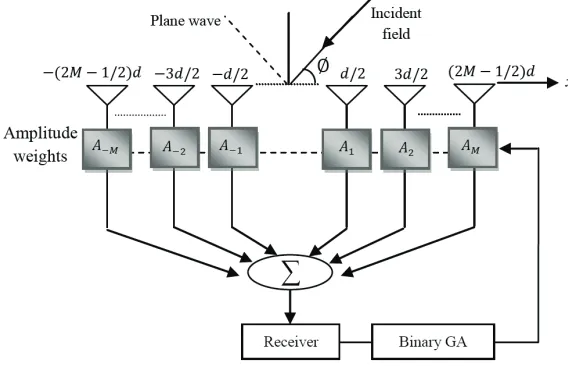
Consider a linear array with uniformly spaced 2M elements as shown in Fig. 2. Unlike the array shown in Fig. 1, the array in the proposed method is weighted with a series of coefficientsA= [A1, A2, . . . , AM],
and their values are either unity or zero, which means that the weights are binary coefficients applied linearly to the array and represent the amplitude excitation of each element in the array. By setting the weightAm to 1, the corresponding element becomes active, i.e., its status is on. On the other hand,
when the value of weight is chosen to be 0, the corresponding element becomes inactive or off, and it does not contribute to the array radiation pattern.
Turning off some elements randomly from the original array introduces non-periodic spacing between the array elements. The non-uniformly spaced arrays have some advantageous over the uniformly spaced arrays. As mentioned previously, not all elements in the array need to be optimized to generate the required nulls. Then the problem becomes how to appropriately select a specific subset of the array elements for thinning in order to accomplish a required goal.
Referring to the array that shown in Fig. 2, its array factor can be given by
AF(u) = 2
M
m=1
Amcos [(n−0.5)kdu] (4)
Note that due to the symmetrical property of the considered array, the number of optimization parameters is equal to M. As mentioned previously that the concept of null steering could be accomplished by a limited number of elements (this is only true if the total number of the interfering signals is smaller than the number of the selected elements). Here we assume that this assumption is true, thus, not all of theM elements are needed to be optimized or thinned. By doing this, not only the array’s structure is simplified, but also the convergence time of the optimizer could be greatly shortened which is an important point in the practical implementation.
preserved during the thinning or optimization process.
Unlike the fully thinned arrays, the number of optimization parameters (i.e., dimension of the optimization problem) in the proposed array is reduced from M variables to only M −L−1. In this regard, it is also worthy to mention that the total number of possible combinations to exhaustively search by the optimizer is reduced from 2M to only 2M−L−1. To highlight this important point, take for exampleM = 50 elements andL= 30 elements, then the total number of combinations that should be searched by the binary GA is equal to 229 instead of 250 Clearly, this significantly shortens the convergence time of the optimization algorithm while maintaining the same capability for interference suppression.
The subset of M −L−1 elements could be selected from anywhere of the original array. Thus, various configurations exist where the designer may select the adjustable subset from inner (center) elements or outer elements of the original array. Choosing the inner elements will turn off some elements located near the center of the array. This means that the corresponding aperture distribution will have a minimum value near the center and a maximum value near the ends. Clearly, such a distribution will produce an undesirable high sidelobe level in the resulting array pattern.
The subset of M−L−1 elements can also be selected randomly from array of M elements. This selection has less influence on the generated nulls, and it is found that the depth of the produced null is not deep enough. On the other hand, the outer element selection is found to have a great influence on the generated nulls, and the depth of the produced nulls is satisfactory. This observation is consistent with the results of [23] in which the nulls were controlled by adjusting the elements at the ends of the array.
Figure 2. Block diagram of the proposed null steering method.
4. SIMULATION RESULTS
Nevertheless, other configurations could also be selected with the proposed approach. A number of scenarios with various configurations and different numbers of elements are presented in the following. In all scenarios, the parameters of the binary genetic algorithm are chosen as: population size of 20; selection is roulette; crossover is single point; mutation rate is 0.15; mating pool is chosen to be 4.
In the first example, the angle of arrival of the interfering signal is assumed at u = 0.21. To effectively suppress this interfering signal, a wide null centered at u= 0.21 is needed. To achieve this null, two sharp nulls aroundu= 0.21 with small spacing equal to 0.01 are introduced (where the nulls are atu= 0.2 andu= 0.22). In this case, the number of elements in the fixed array subset on each side of the original array is set toL= 46 elements, and thus, only 3 elements (excluding the last element) on each side are optimized. These 3 elements are chosen from the array elements located on the extremes of the array. Note that the last element which is located at the end of the array is also fixed for the
(b) (a)
Figure 3. Optimized array pattern for L = 46, M −L−1 = 3 (a) and corresponding amplitude weights (b).
(b) (a)
also plotted in Fig. 3.
It can be seen that the optimized array with only 2 inactive elements on each side of the array is capable of generating the required null(s). The half power beamwidth (HPBW) of the optimized array is exactly same as that of the original uniform array, i.e., 1.56◦.
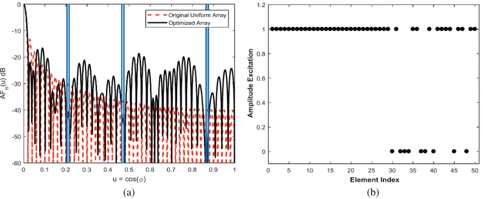
In the second example, three nulls centered at u = 0.21, u= 0.47, and u= 0.87, each with width equal to 0.01, are considered. In this case, the number of elements, L, in the fixed array subset on each side of the array is set to 30, and thus, only 19 elements (excluding the last element) on each side are optimized. Also, these 19 elements are chosen from the outer elements of the original array. Fig. 4 shows the optimized array pattern and the corresponding amplitude weights.
It can be seen that the optimizer turns off 9 elements on each side of the array to generate the required nulls.
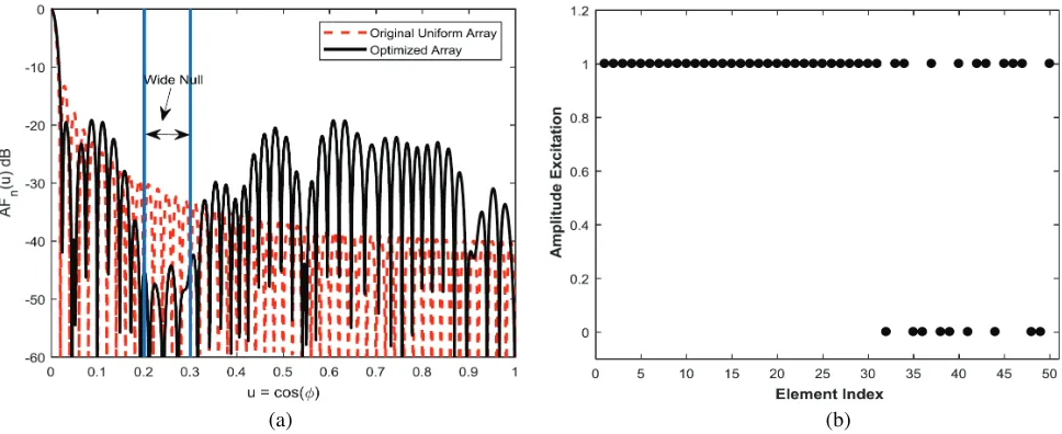
In the third example, a very wide null from u = 0.2 to u = 0.3 is considered. In this case, the number of elements in the fixed array subset on each side of the array is kept same as in the previous
(b) (a)
Figure 5. Optimized array pattern for L = 30, M −L−1 = 19 (a) and corresponding amplitude weights (b).
(d) (c)
Figure 6. Optimized patterns for three different subset elements configurations. (a) Optimized patterns. (b) Amplitude weights of random configuration L = 2. (c) Amplitude weights of inner configurationL= 30. (d) Amplitude weights of outer configuration L= 30.
example. Fig. 5 shows the optimized array pattern and the corresponding amplitude weights.
It can be seen that the sidelobe levels within the range fromu= 0.2 to u= 0.3 are suppressed by more than−45 dB which is quite sufficient to suppress any broadband interfering signal. Although the far sidelobes have increased, the peak sidelobe level is still under−20 dB.
In the next example, the performance of the proposed array under various configurations is considered. As mentioned earlier, the second array subset could be selected from center or outer elements of the array. The optimized elements can also be selected randomly across the array elements. In this specific case, all the array elements should be optimized, andLis equal to 2 elements only (i.e., the first and last array elements on each side of the array are kept constant to keep the overall array length unchanged). Fig. 6 shows the resulting patterns for inner, outer and random configurations with their corresponding amplitude weights, while Fig. 7 shows the convergence speed of the above-mentioned configurations.
two configurations. These results fully confirm the effectiveness of the outer element selection for null steering.
5. CONCLUSIONS
It is shown that by eliminating (or turning off) a subset of active elements in the original uniformly excited arrays, nulls can be accurately pointed toward interfering directions. To find optimally which elements need to be turned off, a binary genetic algorithm is used. Unlike the fully thinned arrays, the proposed null steering method could be accomplished by only selecting a small number of array elements instead of all of them. The proposed array has many advantages compared to the fully thinned arrays such as lower number of optimization parameters, faster convergence speed and lower sidelobe levels. Results show that the proposed method is capable to precisely place single, multiple, and broad nulls toward interfering directions.
REFERENCES
1. Guney, K. and M. Onay, “Amplitude-only pattern nulling of linear antenna arrays with the use of bees algorithm,”Progress In Electromagnetics Research, Vol. 70, 21–36, 2007.
2. Haupt, R. L., “Phase-only adaptive nulling with a genetic algorithm,” IEEE Trans. Antennas Propag., Vol. 45, No. 6, 1009–1015, Jun. 1997.
3. Mohammed, J. R., “Element selection for optimized multi-wide nulls in almost uniformly excited arrays,” IEEE Antennas and Wireless Communication Letters Digital Object Identifier, 10.1109/LAWP.2018.2807371, Feb. 2018.
4. Morgan, D., “Partially adaptive array techniques,”IEEE Trans. Antennas Propag., Vol. 26, No. 6, 823–833, Nov. 1978.
5. Mohammed, J. R. and K. H. Sayidmarie, “Performance evaluation of the adaptive sidelobe canceller with various auxiliary configurations,” AE ¨U International Journal of Electronics and Communications, Vol. 80, 179–185, 2017.
6. Mohammed, J. R., “Optimal null steering method in uniformly excited equally spaced linear array by optimizing two edge elements”,Electronics Letters, Vol. 53, No. 13, 835–837, Jun. 2017. 7. Mohammed, J. R. and K. H. Sayidmarie, “Null steering method by controlling two elements,”IET
Microw. Antennas Propag., Vol. 8, No. 15, 1348–1355, 2014.
8. Mayhan, J. T., “Thinned array configurations for use with satellite based adaptive antennas,”IEEE Trans. Antennas Propag., Vol. 28, No. 6, 846–856, Nov. 1980.
9. Rocca, P., R. L. Haupt, and A. Massa,“ Interference suppression in uniform linear arrays through a dynamic thinning strategy,”IEEE Trans. Antennas Propag., Vol. 59, No. 12, 4525–4533, Dec. 2011. 10. Toso, G., C. Mangenot, and A. G. Roederer, “Sparse and thinned arrays for multiple beam satellite applications,” Proc. Eur. Conf. Antennas Propag. (EuCAP 2007), 1–4, Edinburgh, England, Nov. 11–16, 2007.
11. He, J., D.-Z. Feng, and N. H. Younan, “Optimizing thinned antenna array geometry in MIMO radar systems using multiple genetic algorithm,” IEEE CIE International Conference on Radar, Chengdu, China, Oct. 24–27, 2011.
12. Haupt, R. L., “Thinned arrays using genetic algorithms,”IEEE Trans. Antennas Propag., Vol. 42, No. 7, 993–999, Jul. 1994.
13. Viani, F., L. Lizzi, M. Donelli, D. Pregnolato, G. Oliveri, and A. Massa, “Exploitation of parasitic smart antennas in wireless sensor networks,” Journal of Electromagnetic Waves and Applications, Vol. 24, No. 7, 993–1003, 2010.
15. Caorsi, S., M. Donelli, A. Lommi, and A. Massa, “Location and imaging of two-dimensional scatterers by using a particle swarm algorithm,” Journal of Electromagnetic Waves and Applications, Vol. 18, No. 4, 481–494, 2003.
16. Quevedo-Teruel, O. and E. Rajo-Iglesias, “Ant colony optimization in thinned array synthesis with minimum sidelobe level,”IEEE Antennas Wireless Propag. Lett., Vol. 5, No. 1, 349–352, Dec. 2006. 17. Keizer, W. P. M. N., “Linear array thinning using iterative FFT techniques,” IEEE Trans.
Antennas Propag., Vol. 56, No. 8, 2257–2260, Aug. 2008.
18. Singh, U. and T. S. Kamal, “Optimal synthesis of thinned arrays using biogeography based optimization,” Progress In Electromagnetics Research M, Vol. 24, 141–155, 2012.
19. Donelli, M., A. Martini, and A. Massa, “A hybrid approach based on PSO and Hadamard difference sets for the synthesis of square thinned arrays,” IEEE Trans. Antennas Propag., Vol. 57, No. 8, 2491–2495, Aug. 2009.
20. Caorsi, S., A. Lommi, A. Massa, and M. Pastorino, “Peak sidelobe level reduction with a hybrid approach based on GAs and difference sets,”IEEE Trans. Antennas Propag., Vol. 52, No. 4, 1116– 1121, Apr. 2004.
21. Donelli, M., “Design of broadband metal nanosphere antenna arrays with a hybrid evolutionary algorithm,”Optics Letters, Vol. 38, No. 4, 401–403, Feb. 15, 2013.
22. Febvre, P. and M. Donelli, “An inexpensive reconfigurable planar array for Wi-Fi applications,”
Progress In Electromagnetics Research C, Vol. 28, 71–81, 2012.
23. Tseng, F. I., “Design of array and line-source antennas for Taylor patterns with a null,” IEEE Trans. Antennas Propagat., Vol. 27, 474–479, Jul. 1979.
24. Pogorzelski, R. J., “On a simple method of obtaining sidelobe reduction over a wide angular range in one and two dimensions,”IEEE Trans. Antennas Propag., Vol. 49, No. 3, 475–482, Mar. 2001. 25. Sayidmarie, K. H. and J. R. Mohammed, “Performance of a wide angle and wideband nulling