A Grassmann graph embedding framework for gait analysis

R E S E A R C H

Open Access

A Grassmann graph embedding framework for

gait analysis

Tee Connie

, Michael Kah Ong Goh

and Andrew Beng Jin Teoh

Abstract

Gait recognition is important in a wide range of monitoring and surveillance applications. Gait information has often been used as evidence when other biometrics is indiscernible in the surveillance footage. Building on recent advances of the subspace-based approaches, we consider the problem of gait recognition on the Grassmann manifold. We show that by embedding the manifold intoreproducing kernel Hilbert spaceand applying the mechanics of graph embedding on such manifold, significant performance improvement can be obtained. In this work, the gait recognition problem is studied in a unified way applicable for both supervised and unsupervised configurations. Sparse representation is further incorporated in the learning mechanism to adaptively harness the local structure of the data. Experiments demonstrate that the proposed method can tolerate variations in appearance for gait identification effectively.

1 Introduction

The use of CCTV video cameras for surveillance is common in public and commercial establishments like banks, shopping malls, parks, and railway stations. Most of the current video surveillance systems require human operators to constantly supervise the cameras. In other words, the effectiveness of the system is largely dependent on the vigilance of the person monitoring the system. To resolve this shortcoming, research is under way to develop automated systems for real-time cameras monitoring. Among the efforts, gait recognition is a popular study for automatic human identification. Gait recognition is a biometric technology that identifies people based on the manner they walk. This technology is suitable for person identification at a distance when other biometrics like face, iris, or fingerprint might be obscured or at too low a resolution. In many situations, gait is the only evidence available from a crime scene [1].

With the advent of visual surveillance, it is not difficult to obtain multiple-viewpoint shot of a subject or video outputs over a period of time. These multiple sets of images can be combined to yield better performance as compared to single-shot images. Subspace-based ap-proaches have been shown effective in modeling data

consisting of multiple sets of images [2]. For example, Jacobs et al. [3] showed that illumination on human faces can be modeled as a nine-dimensional subspace under mild assumptions. Subsequent to this finding, sets of images of the same person under varying light-ing conditions are often modeled as low dimensional subspaces [4-6]. While a subspace is a linear space, the collection of linear subspaces is a completely dif-ferent space known as the Riemannian manifold [7]. More formally, the d-dimensional subspace in ℝn is called the Grassmann manifold, named after the famous mathematician Hermann Günther Grassmann [8]. The Grassmann manifold has long been known for its fas-cinating mathematical properties. However, its applications in computer vision and machine learning have appeared rather recently.

Turaga et al. [9] demonstrated the use of computer vision applications such as video-based face recognition, activity recognition, and image set-based object recog-nition on the Grassmann manifold. The Grassmann manifold structure of the face shape is also utilized in [10] for age estimation and face verification. In [11], geometrical structure of the Grassmann manifold was exploited for visual tracking scheme.

Hamm and Lee [12] showed that using a suitable Grassmann kernel, the Grassmann space can be embedded to a higher-dimensional reproducing kernel Hilbert space * Correspondence:[email protected]

2

School of Electrical and Electronics Engineering, College of Engineering, Yonsei University, Seoul, South Korea

Full list of author information is available at the end of the article

(RKHS) where many Euclidean algorithms can be gen-eralized. Subsequent to this finding, several studies extended the use of dimension reduction methods on the Grassmann manifold [13,14]. Considerable improvement in recognition accuracy has been reported for this application.

In this paper, we propose an approach calledGrassmann graph embedding (GGE) for gait analysis. Motivated by the success of the graph embedding (GE) framework [15], we show how GE can be integrated in the Grassmann manifold for the gait recognition problem through the use of well-defined kernel functions on the manifold. We provide a general formulation that supports both supervised and unsupervised dimension reduction mecha-nisms. We further attach semantic meaning to the gait data by incorporating sparse representation in our learning mechanism.

The rest of the paper is organized as follows. In Section 2, we review the different approaches to gait recognition. In Section 3, we provide the background of the methods used in this paper. The overall framework for the pro-posed Grassmann GE learning is described in Section 4. In Section 5, we present experimental results on different settings. Lastly, some concluding remarks are given in Section 6.

2 Related work

We provide a background study for the methods addressing view angle, clothing, and also speed factors in gait recogni-tion. Besides, some subspace-based techniques related to our work are also reviewed in this Section.

2.1 Gait recognition under various viewing angles

Appearance change due to varying view angles is one of the greatest challenges in gait analysis. Studies show that single-view gait recognition performance drops when the view angle changes [16,17]. Current approaches to gait recognition under various viewing angles can be classified into one of the three major categories: (1) extraction of view-invariant gait feature, (2) generation of three-dimensional (3D) gait information, and (3) learning projection or mapping functions to transform gait features from various views into a common feature space.

The first approach attempts to find gait features that are invariant to view changes. Jean et al. [18] introduced body part trajectories as the view-invariant feature. The 2D trajectories of the feet and head were normalized to make them appear as if they were always seen from the front-to-parallel viewpoint. A method was proposed by Kale et al. [19] to synthesize the lateral view from arbitrary view through perspective projection in a sagittal plane. Recently, Goffredo et al. [20] derived gait fea-tures based on estimated joint positions. A reconstruction

method was employed to normalize the gait features from different viewpoints into the side plane. The methods in the first category can only work with limited range of view angles, and the accuracy of the methods can be affected by self-occlusion.

The methods in the second category integrate 3D infor-mation from multiple cameras to construct a gait model. An image-based rendering method was employed by Bodor et al. [21] to reconstruct the 3D view of the subject from a blend of different views. Zhao et al. [22] used video sequences acquired by multiple cameras to setup a human 3D model. Matching for the 3D models was performed using a linear time normalization technique. Yamauchi et al. [23] captured the body data using a high-resolution projector-camera system. They were able to obtain fairly accurate reconstructed synthetic human poses. The methods in the second category are able to provide reliable performance. However, these 3D analysis methods require complicated setup of a calibrated multi-camera system. Besides, these methods demand complex computation which makes them unsuitable for practical application.

The methods in the third category have some learnt mapping/projection function to normalize the gait fea-tures obtained from various viewing points to a shared feature space. Makihara et al. [24] extracted a frequency-domain gait feature using Fourier analysis. After that, a view transformation model (VTM) was used to learn a mapping function for the gait features obtained from different views. Some other variations based on VTMs had also been introduced [25-27]. Studies that utilize VTM [24-27] assume that the feature matrix in the training set can be completely decomposed into view and subject independent submatrices without overlapping elements. However, the view angle may sometimes be difficult to obtaina priori.

In [28], the correlation of gait sequences from different views was modeled using canonical-correlation analysis

(CCA). The CCA strengths were directly used to match two gait sequences. Lee and Elgammal [29] presented a multi-linear generative model using higher-order singular value decomposition. View factors, body configuration factors, and gait-style factors could be obtained using such model. The methods in the third category generate more stable gait features and are less sensitive towards noise as compared to the methods in the first category. Fur-thermore, the methods in the third category deploy a simpler camera setup as compared to those in the second category.

[30] shows that gait spoofing is possible by imitating the clothing of a person with similar build. These observations imply that the clothing factor yields high intraclass vari-ation and low interclass varivari-ation which makes personal identification difficult.

Hossain et al. [31] attempted to address the clothing factor in gait recognition by proposing an approach to adaptively assign weights to different body parts based on how much that area is affected by clothing variation. For example, the head will usually be affected if a person wears a hat, while the leg will be affected if the person wears a long skirt. The algorithm assigns less weight to the head when the person wears a hat and similarly assigns less weight to the leg when the person wears a long skirt. This method thus reduces the influence of clothing by the adaptive weight tuning mechanism. However, the method makes strong assumption on the types of cloth-ing the person wears (e.g., the clothcloth-ing types must be known beforehand), and this makes it not very practical in real-life application.

Another study [32] approached the clothing factor using a random subspace method. Multiple subspaces were randomly formed using the coefficients generated by 2DPCA. A promising result was obtained as the method combined the evidences from multiple subspaces which provided different information about the clothing aspects when classification was performed.

There is also a group of researchers who introduced the use of gait energy image (GEI) with sway alignment [33] to overcome the clothing and carrying effects. In-stead of taking the whole body to generate GEIs, only the area below the knee was used. The authors claimed that their method produced better accuracy as they believed that the lower part of the body was usually unaffected by the clothing and carrying conditions. Nevertheless, this method easily fails when the person's leg is ob-scured (e.g., the person wears a long skirt or carries a briefcase).

2.3 Gait recognition across various walking speeds The approaches towards speed factor in gait recognition bear some resemblance to those methods addressing viewpoint variation. There are two general approaches that deal with gait with varying speeds: (1) learning map-ping functions to transform the gait features from various speeds into a common walking speed and (2) extraction of speed-invariant gait feature. In the first approach, Tanawongsuwa and Bobic [34] proposed a stride nor-malization technique to transform the gait feature across various speeds into a common walking speed. On the other hand, Tsuji et al. [35] viewed cross-speed gait recog-nition as a similar problem as cross-view gait recogrecog-nition and applied the VTM [24] technique to transform the gait from different speeds to a common speed for recognition.

In the second approach, Kusakunniran et al. [36] showed that the use ofProcrustes shape analysiscould tolerate the gait changes due to speed differences. They extended the technique to a higher-order shape config-uration that could better represent the gait signature across speeds. They further introduced a differential com-position model to assign different weights to different shape boundary to cope with large changes in walking speeds. Liu and Sarkar [37] proposed apopulation hid-den Markov modelto normalize the gait features based on a generic walking model. The proposed model, when combined withlinear discriminant analysis, could dis-tinguish the shapes of different subjects and suppress the differences of the same subject under various condi-tions, including speed changes. Tan et al. [38] represented the gait features using eight projective representations. The representation using projection from different di-rections yielded acceptable accuracy for gait recognition across speeds. Recently, Guan and Li [39] deployed the random subspace method [32] to address the cross-speed problem. This method also seemed to respond well towards speed changes.

2.4 Subspace-based approaches

In the computer vision community, the subspace method [40] has been used to represent an image set by a linear subspace that is spanned by all the images in the set. A number of algorithms have been proposed to measure the distances/similarities among the subspaces. Among the many distance/similarity measures, the concept of principal angle [41] between two subspaces has been widely adopted due to its efficient, accurate, and robust characteristics. Yamaguchi et al. [42] presented a method calledmutual subspace method(MSM) that directly used the angles between two subspaces as the similarity score of two face image sets. Li et al. [43] further introduced the idea of weighted subspace distance to more effect-ively account for the characteristics of the underlying data distribution. This method was adopted by Liu et al. [44] in gait recognition to compare two subspaces com-prising gait images captured from different view angles. A nonlinear extension of the principal angle method has also been presented in [45,46].

correlations of within-class sets. This method was shown to perform well in several object recognition problems.

2.5 Motivation and contribution

The subspace-based approach is shown to be promising in modeling video sequences. Subspaces can accommo-date the effect of a wide range of variations and capture the dynamic properties in the video sequences. In many video surveillance applications, multiple snapshots of the same subject at different time instances can be obtained for recognition. Similarly, multiple images of the same subjects under varying viewpoints are also available in video camera networks. Therefore, it is natural to utilize these multiple sets of images instead of the conventional single snapshot image in our recognition task.

Clearly, the subspace-structure data resides on a non-linear manifold. The non-Euclidean domain which suits the subspace-structure data is the Grassmann manifold. The Grassmann manifold G(m, D) is the set of m -dimensional linear subspaces of the ℝD. Hence, a set of linear subspaces can be perceived as points on the Grassmann manifold. Most of the computer vision al-gorithms are developed for data lying inℝD. Applying these algorithms directly on the nonlinear manifold will yield poor accuracy as the underlying geometry of the manifold is ignored. Therefore, this paper aims to generalize the algorithm developed for ℝD to the Grassmann manifold through the use of well-defined Grassmann kernels.

Our primary contributions in this paper are (1) a for-mulation for modeling gait subspaces on the Grassmann manifold, (2) a framework to integrate supervised and unsupervised GE techniques in the Grassmann manifold, (3) a method to incorporate sparse representation in the learning algorithms, and (4) extensive experiment to corroborate the proposed approach.

A preliminary version of this paper was presented in [50], which explored the use of gait recognition on the Grassmann manifold. This paper provides the road block for modeling gait image sets on the Grassmann manifold. A local-based discriminant analysis method calledGrassmann locality preserving discriminant ana-lysis was deployed, and an encouraging result was reported. In this paper, we provide a more detailed ana-lysis and present a framework to integrate supervised and unsupervised GE methods. On top of that, we also propose three graph learning mechanisms, namely glo-bal, local, and adaptive learning, which operate around the GE framework which was not studied in the previous paper.

3 Preliminaries

Brief reviews of the Grassmann manifold and sparse representation are provided in this section. The theory

behind the Grassmann kernel would be helpful to under-stand how points on the manifold could be measured. Some background knowledge of sparse representation would be beneficial in understanding how adaptive learning is accomplished in this work.

3.1 Grassmann manifold

The geometric property of the Grassmann manifold has received significant attention, and a good introduction for this topic can be found in [7]. For image set matching problem, an image set comprising of m images, with each image having D pixels, can be represented as a point onG(m,D). Two points on the Grassmann mani-fold, which correspond to two image sets, are equivalent if one can be mapped to the other by anm×morthogonal matrix [7].

The distance between two subspaces can be measured by canonical distance, which is the length of geodesic path connecting two points on the Grassmann manifold. However, it is more computationally efficient to compute the distances between the subspaces using the principal angles [51]. Given two subspaces,P1andP2, or referred to as points on the Grassmann manifold, principal angles are related to the geodesic distance by

D2_GeoðP1;P2Þ ¼

(Pi) and span (Pj). Principal angles can be conveniently computed usingsingular value decompositionas

P₁0P2¼USV0 ð2Þ

where U= [u1…um], uk ∈ span (P1), V= [v1…vm], vk ∈ span (P2), andSis the diagonal matrixS= diag (cosθ1…

cosθm).

Various distances have been defined based on the principal angles, and some well-known distances are the Binet-Cauchy, projection, and Procrustes distances. Among the various distances, the projection distance, Binet-Cauchy distance, and canonical-correlation distance (the largest principal angle) are induced from positive definite kernels. This means that we can define the corresponding kernels on the Grassmann manifold based on these matrices.

In this paper, the projection kernel and canonical-correlation kernel are adopted as they are reported to provide good result [12,14]. Given two points on a Grassmann manifold, Xi and Xj ∈ ℝDxm, the similarity between the points is defined as

subject toaT_pap ¼bTpbp ¼1 andaTpaq¼bTpbq¼0,p≠q;

k_proj denotes the projection kernel while k_cc signifies the canonical-correlation kernel.

3.2 Sparse representation

In the past few years, sparse representation (SR) has proven to be a powerful tool for computer vision, com-putational biology, statistics, pattern recognition, and other applications [32,52,53]. Given a signal, or the col-umn vector of an image in our case,xi∈ℝkand an over-complete dictionary [54] withkbases,X= [x1,x2,…,xn]∈ ℝn×k

(k>n), the goal of SR is to representxiusing as few entries of X as possible. The objective function can be defined as follows:

minkSik0s:t:xi¼XSi ð5Þ

where Si denotes the sparse coefficient matrix and ∥∙∥0

denotes thel0norm of a vector.

However, it is NP-hard to find the sparsest solution for Equation 2 using l0-minimization. As such, l1 -minimization is often used to solve the problem [54]. In practical applications, there might be noises in signalxi. Therefore, the following optimization model is used to estimateSi:

minkSik1s:t:kxi−XSik2<ε ð6Þ where∥∙∥1isl1-norm andεis the error-tolerant term. 4 Proposed approach

The detail of the proposed approach is given in this section. The proposed method mainly consists of three stages: GEI construction, Grassmann projection, and GGE. Two types of GGE configurations are introduced: supervised and unsupervised. Three different graph learning mechanisms are further presented for each of the GGE learning modes. The general framework for the proposed approach is depicted in Figure 1.

4.1 Gait energy image

The simple yet effective GEI [55] approach is deployed in this paper. Given a gait sequence fItð Þi;j gFt¼1, where

It(i,j) is a pixel at position (i,j) in the imageIt, andFis the total number of frames in the gait sequence, GEI is defined as

GEIð Þ ¼i;j X

F

t¼1

Itð Þi;j =F: ð7Þ

One advantage of representing the gait feature using GEI is that we do not need to consider the underlying dynamics of the walking motion. This representation enables us to study the gait sequence from a holistic

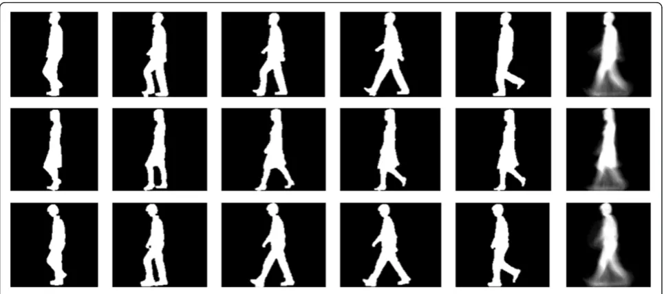
view by implicitly characterizing the structural statistics of the spatiotemporal patterns of the walking person. The original silhouette images and the resulting GEI images of three subjects are illustrated in Figure 2. We observe that the subjects can be favorably distinguished from the GEI images.

4.2 Grassmann projection

The set of GEI images taken from the video sequence are modeled as a collection of linear subspaces. In this way, the undesired variability due to view angle, pose, and appearance changes can be absorbed within subspaces, and the variability of subject identity can be emphasized as variability among the subspaces. Most subspace-based learning techniques [4-6] employ an inconsistent mechan-ism, e.g., feature extraction is performed in the Euclidean space while non-Euclidean subspace distances are used. Optimization and convergence will be difficult to achieve using this inconsistent approach [12]. Under the Grassmann framework, the feature extraction and distance meas-urement can be integrated in a graceful manner, resulting in a simpler and more familiar algorithm.

Given sets of GEIs calculated using Equation 7, we com-pute SVD over the image sets to obtain the corresponding subspaces{X1,X2,…,Xn} whereXi∈ℝDxmandDrefers to the length of the gait feature while m signifies the number of images comprising the subspaces. After that, the Grassmann kernel is applied on these subspaces. To this end, we have tested two types of kernel functions, namely the projection and canonical kernels [12,14] given in Equations 3 and 4.

4.3 Grassmann graph embedding

Grassmann kernels allow us to embed the manifold in a higher-dimensional RKHS to which many Euclidean algo-rithms can be generalized. Conventional dimension reduc-tion techniques like linear discriminant analysis (LDA), principal component analysis (PCA), and locality preserving projection (LPP) can thus be applied on the Grassmann manifold to further improve recognition accuracy [12-14]. The GE framework [15] has proven to be effective in unify-ing the various dimension reduction algorithms. Given points from the underlying Grassmann manifold ℳ, the local geometrical structure ofℳ can be modeled by con-structing a similarity graphW. LetG= {V,W} denotes an undirected weighted graph with vertices Vand similarity matrixW. The values forWcan be directly obtained from the output of the Grassmann kernel. On the other hand, the diagonal matrixDand the Laplacian matrix L of the graphGare defined asL=D–WwhereDii¼

X

j≠i

Wij:

between vertex pairs in the original high-dimensional space. The solution can be directly obtained using eigenvalue decomposition [15]. In the following text, we formulate the GE dimension reduction problem over the Grassmann manifolds for unsupervised and supervised configurations.

The unsupervised GGE approach is suitable for open surveillance systems like applications to monitor pe-destrians at the streets and customers at the shopping

malls. It is very difficult, if not impossible, to obtain the subject's identity in such settings; thus, unsuper-vised GGE will be useful in discerning an individual with unknown identity. On the contrary, supervised GGE is appropriate for closed-set identification like monitoring employees in a workplace. As the identity of the legitimate subject is known, supervised GGE would be able to classify the gait data reliably using identity information.

Figure 2Samples of original silhouette images and the resulting GEI images.

Supervised Non-Supervised

Ww Wb _{Ww Wb}

Ww Wb

Global Local

Adaptive

Global Local Adaptive

Grassmannian Graph Embedding GEI

construction

Grassmannian Projection Input video

sequence

W W W

Class 1

Class N

4.3.1 Unsupervised GGE

We formulate the unsupervised GGE method by first forming the similarity graph W. We want to find a mapping function F:Yi→Zi to map the points on the Grassmann manifold, ℳ, to a new manifold, ℳ’, to preserve the local geometry of the manifold. In other words, we want to find a transformation which maps the connected points on W as close as possible. The following objective function realizes this criterion:

minX ij

Zi−Zj

2

Wij: ð8Þ

The objective function Wij incurs a heavy penalty if the connected neighbors are mapped far apart in ℳ’. Therefore, minimizing Wij ensures that Zi and Zj are close ifYiandYjare close.

Suppose U is a projection matrix,ZT= UTY, that ful-fills the objective function (8) andYis the kernel matrix produced by the Grassmann kernel. By simple algebra manipulation, the objective function can be reduced to

1=2X

whereDis a diagonal matrix given by Dij¼

X

j

Wij. The optimization problem can be reduced to finding

arg min

The projection matrix U that minimizes Equation 8 is given by the maximum eigenvalue solution to the gener-alized eigenvalue problem:

YLYTU¼λYDYTU: ð11Þ

4.3.2 Supervised GGE

The unsupervised GGE method can be extended to the supervised version by constructing two similarity graphs, Ww,ij and Wb,ij, which denote the within-class and between-class similarity matrices, respectively. The extension is desirable as we can take advantage of the class label information to improve the classification accuracy. The mapping function for supervised GGE is slightly different from its unsupervised counterpart. The new mapping function F0:Yi →Zt0 is formed such that the

connected points of the within-class similarity matrix,

Ww,ij, stay as close as possible while connected points of the between-class similarity matrix,Wb,ij, stay as distant as possible. The class label information is used in this

method to discover the discriminant structure of the samples. The objective functions for supervised GGE are defined as follows:

The objective functionWw,ijincurs a heavy penalty if neighboring points Z0_i and Z0_j are mapped far apart while they are actually in the same class. Likewise, the objective functionWb,ijincurs a heavy penalty if neigh-boring points Z0_i and Z0_j are mapped close together while they belong to different classes.

Suppose U is a projection matrix, Z0T = UTY, to realize the objective functions (12) and (13). By simple algebra manipulation, the objective function (12) can be reduced to Similarly, the objective function (13) can be condensed to the following form:

Wb;ij. The optimization problem can be condensed into the following form:

The projection matrix that minimizes Equation 16 can be obtained by solving the generalized eigenvalue problem:

YLbWwU¼λYDwYTU: ð17Þ

4.3.3 Constructing the similarity graphs

Graph relations play a crucial role in the GE framework to determine how the methods behave based on the connectiv-ity and weight assignment of the neighboring points in the data. We present three approaches for graph construction: global, local, and adaptive. The first approach constructs fully connected graphs where all nodes are connected using predefined weights. The representative methods for this approach are PCA and LDA for unsupervised and supervised configurations, respectively.

The second approach takes into consideration the neighborhood information where only thekneighboring nodes are connected in the graph. If k=N, the local ap-proach is the same as the global apap-proach. Some popular methods for this approach are LPP and locality preserving discriminant analysis [56] for unsupervised and supervised modes, respectively.

The third approach adaptively assigns weights to the nodes based on how the rest of the samples contribute to the sparse representation of the nodes. This is an unconventional approach for graph construction, and the detail of constructing the adaptive graph is given in the subsequent section.

Weight assignment for the similarity graphs for the global approach is straightforward where all nodes in the graph are connected with equal weights. For the unsuper-vised mode, the simplest graph structure is to setWij=1. Another way to form the similarity graph is using the heat kernel equation Wij¼ −x^i−^xjk2=t

[15] wheretis an adjustable constant. In contrast to the unsupervised mode, two graphs are constructed in the supervised mode. Weights are assigned to the within-class similarity graph,

Ww,ij, if two nodes share the same class label; 0 otherwise. Similarly, weights are assigned to the between-class

similarity graph, Wb,ij, if two nodes are not from the same class; 0 otherwise.

For the local approach, the simplest graph structure is the simple-minded graph where the similarity matrixWij is set to 1 if^xi is among thekth nearest neighbors of^xj;

0 otherwise. The weight can also be replaced by the heat kernel equation. On the other hand, the supervised method takes into consideration the class information and sets the within-class similarity graphWw,ij= 1 if^xiis among thekth

nearest neighbors of x^j in the same class;0 otherwise. In a

similar manner, the between-class similarity graph assigns

Wb,ij= 1 if x^i is among thekth nearest neighbors of ^xj in

different classes; 0 otherwise.

We also propose a self-adaptive graph structure. Suppose

S(i, j) is the sparse output estimated by Equation 6 using the column vector of X^ (output of the Grassmann kernel), the similarity graph for unsupervised self-adaptive graph is defined asWij=S(i,j). On the other hand, the within-class similarity graph for the supervised method is defined as

Ww,ij=Sw(i, j).Sw is the output from Equation 6 fulfilling the conditions ^xi∈Nw ^xj or ^xi∈Nw ^xj whereNw ^xj is

the set ofkneighbors sharing the same label with ^xi. The

between-class similarity graph is characterized byWb,ij=Sb (i,j).Sbis the output from Equation 6 andx^i∈Nb ^xj or ^

xj∈Nbð Þ^xi whereNbð Þ^xi is the set ofkneighbors having

different labels. This is the basic approach to construct an adaptive graph where a single dictionary is learnt for all classes. Since the dictionary is learnt only once, some computational burden can be saved.

A number of variations can be derived from this basic idea. For example, class-specific dictionary can be learnt where each class is modeled independently of the others.

Wwcan be modeled from the SR output using the column vector ofX^w, whereX^w is the Grassmann output sharing

the same labels with the test sample.Wbcan also be con-structed using the SR output using the column vector of

^

Xb, where X^b is the Grassmann output having different

labels with the test sample. This approach enables the learnt dictionary to have an efficient representation for each class. However, dictionary learning has to be performed multiple times for different classes.

If one wishes to uncover only the semantic information in the between-class similarity graph (due to the fact that per-haps not much interesting information can be revealed in the sparse within-class similarity graph as large values are expected for nodes coming from the same class), the between-class similarity graph could be generated using the sparse approach while the within-class similarity graph be constructed using the simple-minded or heat kernel func-tions. The combination of fully connected and sparse graphs benefits from the flexibility of sparse graph and low compu-tational cost of the fully connected graph. Table 1 summa-rizes the different graph construction methods for GGE.

5 Experiments

Two databases were used to evaluate the proposed method namely, the Chinese Academy of Sciences, Institute of Automation (CASIA) gait database: dataset B [57] and the Osaka University, Institute of Scientific and Industrial Research (OU-ISIR) gait database: datasets A and B [58]. The CASIA gait database is good for assessing the view variation effect on gait as it contains a large number of subjects taken from different viewing angles. The CASIA gait database consists of 124 subjects captured from 11 different angles. The viewing angles range from 0° to 180°, separated by an interval of 18°. There are ten walking sequences for each subject, with six samples containing subjects walking under normal condition, two samples with subjects walking with coats, and two samples with subjects carrying bags. Therefore, there are altogether 13,640 (10 × 11 × 124) gait sequences in the database. All the images were cropped and normalized to 120 × 120 pixels.

The OU-ISIR gait database is suitable for assessing the influence of speed changes and clothing variations on gait. The OU-ISIR gait database: dataset A contains 35 subjects captured from side view with speed variation from 2 to 7 km/h, at an interval of 1 km/h. There are two walking sequences for each speed level. Thus, there are 420 (2 × 6 × 35) gait sequences in this dataset. On the other hand, dataset B is made up of 68 subjects acquired from side view with clothing variations. There are many clothing combinations in this dataset which include pants, half shirt, rain coat, skirt, and cap. All the images for the OU-ISIR database were cropped and resized to 128 × 88 pixels.

5.1 Experiment result

5.1.1 Evaluation on view variations

The CASIA gait database was used to testify the perform-ance of the proposed method under view changes. All the six gait sequences under the normal walking condition were used. For clear indication, each of the viewing angles {0°, 18°, …, 180°} were labeled as θ= {1, 2, …, 11}. We formulated three cases to evaluate the proposed method against viewpoint changes. We simulated realistic scenar-ios where the multiple views could have been acquired from fairly different viewpoints:

1. Same view setting,θtest=θtrain. In this setting, all the

viewpoints used in the training and testing sets were the same, e.g.,θtrain= {1,…, 11} andθtest= {1,…, 11}.

2. Mixed view setting,θtest=θ;θtrain=θ. In this

setting, we made it challenging in which not all the poses in the testing sets were available for training, e.g.,θtrain= {2, 3, 4, 6, 8} andθtest= {2, 4, 6, 7, 9}.

3. Different view setting,θtest=θ−θtrain. This is a

which were totally different from those in the training set, e.g.,θtrain= {2, 4, 6, 9} andθtest= {1, 3, 5, 8}. We

further included more challenging scenarios to test how the proposed method was able to generalize unseen viewpoints, e.g.,θtrain= {1, 2, 3, 4} and θtest= {7, 8, 9, 10}. This is an interesting experiment

to see how well the proposed method performs in extrapolating view angles beyond the known view angles. The previous setting where the estimation of view angles is within the range of known view angles (e.g.,θtrain= {2, 4, 6, 9} andθtest= {1, 3, 5, 8}) can be

seen as an interpolation case.

The following setup was deployed to run the experiment. We randomly selected four gait sequences from each sub-ject to form the training set, and the remaining sequences were for the testing set. The selected view angles for the different settings were modeled as the subspace for each sample in the training and testing sets. We then computed the similarity score for every pair of training–testing matches. The random division of the gait sequences into training and testing sets was repeated several times, and the average result was recorded. The k-nearest neighbor method was used to measure the similarity score between the training and testing sets.

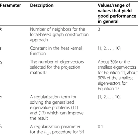
For SR dictionary learning, we deployed thel1-regularized least square problem solver distributed by Boyd's research group [59]. The algorithms are sensitive towards several pa-rameters listed in Table 2. The values or range of values that generally yield good performance based on empirical test are also given in Table 2. The results reported in this paper were obtained based on the best possible combination of the parameters. The rank-1 recognition

rate was used as the performance indicator. The correct match was counted when the sample in the testing set was the best match (top one) from the training set.

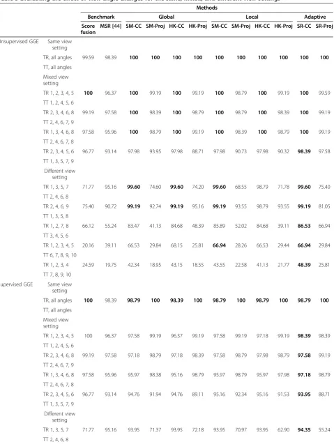
The experimental results for evaluating the changes in view angles are shown in Table 3. The canonical-correlation kernel is denoted as CC, kernel while projec-tion kernel is termed as‘Proj’. The prefixes‘SM’,‘HK’, and ‘SR’ are the abbreviations for simple-minded (the binary graph), heat kernel function, and sparse representation. We included comparison with the multi-view subspace representation (MSR) method. On top of that, we also

Table 2 List of parameters used in GGE

Parameter Description Values/range of

values that yield good performance in general

k Number of neighbors for the local-based graph construction approach

3

t Constant in the heat kernel function

{1, 2,_…, 10}

q The number of eigenvectors selected for the projection matrixU

About 30% of the smallest eigenvectors for Equation11; about 30% of the smallest eigenvectors for Equation17 σ A regularization term for

solving the generalized eigenvalue problems (11) and (17) which can improve the result

{1, 2,…, 10}

λ A regularization parameter for thel1_lsprocedure for SR

0.1

Table 1 Summary of the different graph construction methods

Approach Unsupervised GGE Supervised GGE

Global Wij¼exp −jjW ið Þjj;j

Table 3 Evaluating the effect of view angle changes for the same, mixed, and different view settings

Methods

Benchmark Global Local Adaptive

Score fusion

MSR [44] SM-CC SM-Proj HK-CC HK-Proj SM-CC SM-Proj HK-CC HK-Proj SR-CC SR-Proj

Unsupervised GGE Same view setting

TR, all angles 99.59 98.39 100 100 100 100 100 100 100 100 100 100

TT, all angles

Mixed view setting

TR 1, 2, 3, 4, 5 100 96.37 100 99.19 100 99.19 100 98.79 100 99.19 100 99.59

TT 1, 2, 4, 5, 6

TR 2, 3, 4, 6, 8 99.19 97.58 100 98.39 100 98.79 100 98.79 100 98.39 100 99.19

TT 2, 4, 6, 7, 9

TR 1, 3, 4, 6, 8 97.58 95.96 100 98.79 100 99.19 100 98.39 100 98.79 100 99.19

TT 2, 4, 6, 7, 8

TR 2, 3, 4, 5, 6 96.77 93.14 97.98 93.95 97.98 88.71 97.98 90.73 97.98 90.32 98.39 97.58

TT 1, 3, 5, 7, 9

Different view setting

TR 1, 3, 5, 7 71.77 95.16 99.60 74.60 99.60 74.20 99.60 68.55 98.79 71.78 99.60 75.40

TT 2, 4, 6, 8

TR 2, 4, 6, 9 75.40 90.72 99.19 92.74 99.19 95.16 99.19 93.55 98.79 93.55 99.19 81.05

TT 1, 3, 5, 8

TR 1, 2, 7, 8 66.12 55.24 83.47 41.13 84.68 48.39 85.89 52.02 84.68 39.11 86.53 66.94

TT 3, 4, 5, 6

TR 1, 2, 3, 4, 5 20.16 39.11 66.53 29.84 68.15 25.81 66.94 28.26 66.53 29.44 66.94 29.84

TT 6, 7, 8, 9, 10

TR 1, 2, 3, 4 24.59 19.75 42.34 18.95 43.15 18.55 43.55 22.58 41.13 21.77 48.39 25.81

TT 7, 8, 9, 10

Supervised GGE Same view setting

TR, all angles 100 98.39 98.79 100 98.39 100 98.79 100 98.79 100 98.79 100

TT, all angles

Mixed view setting

TR 1, 2, 3, 4, 5 100 96.37 97.58 99.19 96.37 99.19 97.58 99.19 97.18 99.19 98.39 98.39

TT 1, 2, 4, 5, 6

TR 2, 3, 4, 6, 8 99.19 97.58 97.18 98.79 97.18 98.39 97.58 98.79 97.98 98.79 97.58 99.19

TT 2, 4, 6, 7, 9

TR 1, 3, 4, 6, 8 97.58 95.96 95.97 98.38 95.16 98.79 95.97 98.79 95.97 97.98 97.18 98.79

TT 2, 4, 6, 7, 8

TR 2, 3, 4, 5, 6 96.77 93.14 94.76 91.94 94.76 89.11 95.16 92.34 95.16 91.53 93.95 88.71

TT 1, 3, 5, 7, 9

Different view setting

TR 1, 3, 5, 7 71.77 95.16 93.95 71.37 93.95 72.18 93.95 70.97 93.95 62.90 94.35 55.24

added the classical score-level fusion method to benchmark the algorithm. The scores from the different view angles were fused together using the minimum dissimilarity selection rule [60].

When all of the viewing angles are used to train the system, 100% accuracy could be achieved for all the methods except for score-level fusion and MSR. It is not surprising to get such good result because GGE captures the variations in viewpoint changes when recognition is performed. In the mixed view settings, promising results close to 100% accuracy is obtained. This is encouraging as the proposed methods are shown to possess cross-view capability. The performance is still favorable in the differ-ent view settings when the viewpoints in the testing set are close to that in the training set. However, the accuracy drops when the viewpoints in the testing sets are far apart from the training set (e.g., in the case of TR 1, 2, 3, 4; TT 7, 8, 9, 10). We accept such poor result because we understand that it is a challenging problem to extrapolate unseen views which are very different from the existing views. Based on the results shown in Table 3, we notice that the proposed method using CC kernel consistently yields good results. The effectiveness of SR has been verified in the experiments.

5.1.2 Variants of SR analysis

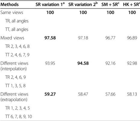
In this experiment, we evaluate the different variants derived from the SR similarity graph construction approach described in Section 4.3.3. Table 4 displays the performance of the different graph combination methods. Adaptive supervised GGE with CC kernel was applied in this ex-periment. SR variation 1 refers to the basic adaptive graph construction approach which learns a shared dictionary for all classes. This method constructs the within-class and between-class similarity graphs usingWw,ij=Sw(i,j) andWb,ij=Sb(i,j). Thel1-minimization algorithm given in Equation 6 is run once per test sample, and the output is split intoWw,ijandWb,ijbased on the class labels.

On the contrary, SR variation 2 learns class-specific dictionary. It builds the within-class similarity graph using

Ww;ij¼^Swð Þi;j where ^Swð Þi;j is the result of running

l1-minimization on the Grassmann output sharing the same class labels with the test sample. The between-class similarity graph is constructed usingWb;ij ¼S^bð Þi;j where ^

Sbð Þi;j is the result of running l1-minimization on the Grassmann output having different class labels from the test sample. In this respect, thel1-minimization algorithm was run twice per test sample: the first time using the training data from the same class to construct Ww,ijand the second time using the training data from the other classes to constructWb,ij.

As for the SM + SR method, the simple-minded function was used to generate the within-class similarity graph,

Ww,ij, while SR was used to build the between-class simi-larity graph, Wb,ij. Likewise, the heat kernel function and SR were used to generateWw,ijandWb,ij, respectively, for the HK + SR method.

Table 3 Evaluating the effect of view angle changes for the same, mixed, and different view settings(Continued)

TR 2, 4, 6, 9 75.40 90.72 93.15 93.15 93.15 92.74 93.55 93.55 93.55 91.94 93.95 84.27

TT 1, 3, 5, 8

TR 1, 2, 7, 8 66.12 55.24 77.02 44.35 76.21 39.52 77.42 47.98 76.21 44.76 78.63 22.98

TT 3, 4, 5, 6

TR 1, 2, 3, 4, 5 20.16 39.11 58.47 18.95 57.66 16.53 59.27 25.81 58.47 27.02 59.27 19.76

TT 6, 7, 8, 9, 10

TR 1, 2, 3, 4 24.59 19.75 37.10 11.29 37.50 11.69 38.31 13.71 37.50 10.89 42.34 13.31

TT 7, 8, 9, 10

The values in bold refer to the highest accuracy rate for each scenario. TR, training set; TT, testing set.

Table 4 Rank-1 recognition rate (%) of the different combinations of SR similarity graphs

Methods SR variation 1a SR variation 2b SM + SRc HK + SRd

Same views 100 100 100 100

TR, all angles

TT, all angles

Mixed views 97.58 97.18 96.77 96.89

TR 2, 3, 4, 6, 8

TT 2, 4, 6, 7, 9

Different views (interpolation)

93.95 94.58 92.16 92.98

TR 2, 4, 6, 9

TT 1, 3, 5, 8

Different views (extrapolation)

59.27 58.47 57.66 58.13

TR 1, 2, 3, 4, 5

TT 6, 7, 8, 9, 10

The values in bold refer to the highest accuracy rate for each scenario.a Learns from a shared dictionary;b

learns from class-specific dictionary;c

combination of simple-minded and SR methods;d

We observe that the performances of the different SR variations do not deviate significantly. We use SR vari-ation 1 in the subsequent sections as it gives slightly better results in most situations. Besides, it is less time-consuming as compared to SR variation 2 and does not require additional parameters like the number of neighborskand the constant termtas compared to SM + SR and HK + SR.

5.1.3 Evaluation on clothing and carrying conditions We conducted experiments to examine the performance of the proposed methods under clothing variations. The main purpose of this experiment is to simulate the condi-tion where suspects captured by the surveillance cameras are trying to masquerade themselves by wearing covers like rain coat or hat. This experiment is also useful to identify the ability of the proposed method to discriminate individuals who wear loose outfits like baggy pants and skirt (for ladies) which can obstruct the gait pattern from being observed properly.

The CASIA and OU-ISIR gait databases were used for this evaluation. For the CASIA database, we took four normal gait sequences as the training set and two bags-carrying and two coats-wearing sequences as the testing sets. All the 11 viewing angles were applied in

the test. Using two types of data for training and testing (one from the normal walking sequence and the other from the carrying/clothing conditions) is a more realistic setting where we need to generalize the unknown carrying/ clothing type from the existing dataset. In real-life scenario, there is no way for us to predict the types of clothes the person wears or the things the person carry when he/she walks. As for the OU-ISIR database, six different clothing combinations were tested. Most of the clothing combina-tions were from types A (e.g., regular pants and parka) to M (e.g., baggy pants and down jacket) [58]. The clothing types were chosen such that we could get the largest pos-sible variations for the test. Only 16 subjects were tested in this experiment. This is because we could only identify 16 corresponding pairs between dataset A, the normal walking sequence, and dataset B, walking with clothing variations. Six sequences from dataset A were used as the training set, while the six sequences in dataset B were used as the testing set.

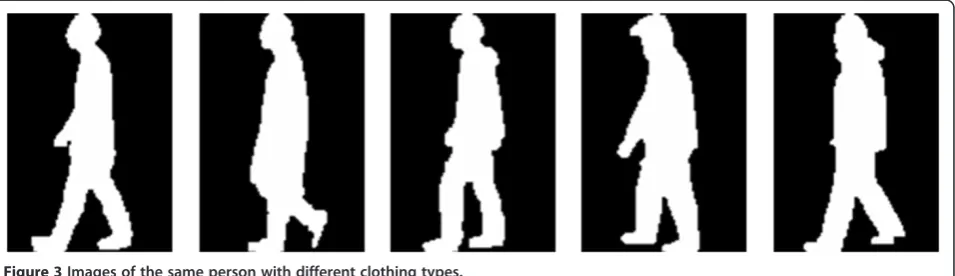
The results of the tests are shown in Table 5. We find that the variations in clothing alter an individual's ap-pearance and make the problem of gait identification challenging. For example, the images depicted in Figure 3 are taken from the same subject. The images look different when different types of clothing are worn. The experiment

Table 5 Evaluating the effect of clothing and carrying conditions

Benchmark Global

method

Local method

Adaptive method

Score fusion

MSR [44] SM-CC SM-Proj HK-CC HK-Proj SM-CC SM-Proj HK-CC HK-Proj SR-CC SR-Proj

Unsupervised Clothing (CASIA) 27.82 19.75 22.98 57.66 23.79 50.00 22.98 57.66 23.79 56.05 20.16 57.56

Clothing (OU) 43.75 43.75 6.25 6.25 6.25 6.25 25.00 6.25 25.00 6.25 50.75 34.25

Carrying condition (CASIA)

89.70 65.32 70.56 77.02 68.95 77.02 70.56 77.02 70.16 84.27 76.77 89.22

Supervised Clothing (CASIA) 27.82 19.75 14.52 58.47 14.92 37.50 15.73 63.31 14.92 59.27 43.71 63.38

Clothing (OU) 43.75 43.75 43.75 18.75 37.50 25.00 43.75 18.75 43.75 12.50 51.50 42.50

Carrying condition (CASIA)

87.90 65.32 47.98 82.26 47.58 58.87 50.40 88.71 49.60 88.71 55.96 89.51

The values in bold refer to the highest accuracy rate for each scenario.

suggests that further investigation has to be carried out to study gait recognition with substantial clothing variations. Nevertheless, the methods could handle the carrying condition satisfactorily.

5.1.4 Evaluation on walking speeds

We have also conducted experiments to assess the effect of walking speed on gait. We are interested in this study as the perpetrator usually walks faster in order to leave the crime scenes immediately. The OU-ISIR gait database was used for this evaluation. Using similar treatment as the view angle evaluation, we labeled the speed {2, 3,…, 7 km/h} as S= {1, 2, …, 6}. Table 6 shows the result of evaluating speed variations. Some methods could achieve 100% accuracy when all the speeds are used. Unlike

clothing variations, speed changes do not drastically affect the accuracy of gait identification. Therefore, the methods could tolerate speed variations quite robustly.

5.2 Summary and discussion

The important findings of this work are summarized below:

The Grassmann manifold provides a platform to reduce the subspace-to-subspace matching problem to a point-to-point matching model. This is immensely useful for gait recognition as the gait video sequences naturally fall in the subspace learning paradigm (unlike face recognition which can be carried out using single image).

Table 6 Evaluating the effect of speed variations using rank-1 recognition rate (%)

Benchmark Global

method

Local method

Adaptive method

Score fusion MSR [44] SM-CC SM-Proj HK-CC HK-Proj SM-CC SM-Proj HK-CC HK-Proj SR-CC SR-Proj

Unsupervised GGE TR, all speeds

97.06 100 100 94.12 100 94.12 100 100 100 100 100 100

TT, all speeds

TR 1, 2, 3 10.29 26.47 35.29 2.94 35.29 2.94 35.29 2.94 35.29 2.94 44.71 26.25

TT 4, 5, 6

TR 1, 2 5.88 14.71 11.76 11.76 11.76 11.76 11.76 11.76 11.76 11.76 23.53 23.53

TT 5, 6

Supervised GGE TR, all speeds

97.06 100 100 94.12 100 94.12 100 94.12 100 94.12 100 100

TT, all speeds

TR 1, 2, 3 10.29 26.47 70.59 11.76 67.64 17.65 70.59 11.76 70.59 11.76 70.65 17.65

TT 4, 5, 6

TR 1, 2 5.88 14.71 29.41 11.76 29.41 8.82 29.41 11.76 35.29 14.71 35.71 8.82

TT 5, 6

The values in bold refer to the highest accuracy rate for each scenario.

The unsupervised and supervised GGE

configurations provide different treatments to gait dataset of different natures (labeled and unlabeled). Nevertheless, the two approaches can be unified gracefully under a general formulation.

GGE outperforms the benchmark methods for all cases. The proposed adaptive learning approach, in particular, yields considerable improvement in classification accuracy.

As a comparison among the different graph construction approaches, the adaptive graph construction method obviously outperforms its counterparts. However, no conclusive remark can be drawn between the global and local methods. The global approach performs better than the local approach under view angle changes, but the opposite happens for the clothing and carrying conditions, while almost similar results were obtained for speed variation. As such, we conjecture that the topological structure of the graph has disparate impact on different scenarios. No single graph structure (referring to the global and local graphs) works best for all cases.

Unsupervised GGE surprisingly outperforms its supervised counterpart in a number of scenarios, e.g., gait image sets with varying view angles and different clothing appearances. The reason why the unsupervised method performs better than the supervised scheme may be because the similarity graphWencodes general information about the relationship among the nodes, whereas the within- and between-similarity graphs,WwandWb, may overlook

some subtle discriminative connection in the graphs. There may also be some outliers in the labeled training set, for example, an image of a person wearing thick sweater with hood that confuses the true appearance of the person, which explains why the supervised method is slightly inferior to the unsupervised method. This counterintuitive result suggests that it might be better to resort to unsupervised method when the cost of labeling the data is high where the class information would not lead to a dramatic improvement in recognition rate.

The canonical-correlation kernel generally performs better than the projection kernel in the changing view scenario. We attribute this to the nature of the canonical-correlation kernel which is based on the notion of principal angle. The canonical-correlation kernel will always find the closest view angle in the training set for comparison. This concept is illustrated in Figure4. Nevertheless, the projection kernel performs better than the canonical-correlation kernel in the clothing and carrying conditions. This may be due to the fact that projection kernel

treats the image subspaces from a more holistic aspect. However, if the sample size is small, e.g., for the OU dataset, projection kernel does not have any advantage over the canonical-correlation kernel. The result suggests that the kernels describe different aspects of the subspaces.

6 Conclusions

This paper demonstrates how it is possible to formulate the gait recognition problem on the Grassmann manifold. This formulation enables us to work in higher-order data structure to harness the nonlinear structure of the data and yet benefit from conventional vector-based computa-tion. We present a method comprising unsupervised and supervised learning modes on the Grassmann manifold. We further introduce the concept of adaptive graph in the learning mechanism to adaptively tailor the graph content based on the nature of the dataset. Experimental results suggest that the proposed method has a potential for practical application as it demonstrates view- and speed-invariant capabilities.

Competing interests

The authors declare that they have no competing interests.

Acknowledgements

This research was partially supported by Ministry of Science and Technology (MOSTI), Malaysia and Basic Science Research Program through the National Research Foundation of Korea (NRF) funded by the Ministry of Science, ICT and Future Planning (2013006574).

Author details

1_{Faculty of Information Science and Technology, Multimedia University,} Malacca, Malaysia.2School of Electrical and Electronics Engineering, College of Engineering, Yonsei University, Seoul, South Korea.

Received: 25 July 2013 Accepted: 2 January 2014 Published: 4 February 2014

References

1. DS Matovski, MS Nixon, S Mahmoodi, JN Carter, The effect of time on gait recognition performance. IEEE Trans. Inf. Forensics and Secur.7(2), 543–552 (2012)

2. W Zhao,Face Processing(Academic Press, Burlington, 2005)

3. R Basri, DW Jacobs, Lambertian reflectance and linear subspaces. IEEE Trans. Pattern Anal. Mach. Intell.25(2), 218–233 (2003)

4. TK Kim, J Kittler, R Cipolla, Discriminative learning and recognition of image set classes using canonical correlations. IEEE Trans. Pattern Anal. Mach. Intell. 29(6), 1005–1018 (2007)

5. H Cevikalp, B Triggs, Face recognition based on image sets, in2010 IEEE Conference on Computer Vision and Pattern Recognition, CVPR 2010 (IEEE, Piscataway, 2010), pp. 2567–2573

6. R Wang, S Shan, X Chen, W Gao, Manifold-manifold distance with application to face recognition based on image set, in2008 IEEE Conference on Computer Vision and Pattern Recognition, CVPR2008(IEEE, Piscataway, 2008), pp. 1–8

7. A Edelman, TA Arias, ST Smith, The geometry of algorithms with orthogonality constraints. SIAM J Matrix Anal. Appl.20(2), 303–353 (1999) 8. Wikipedia, Hermann Grassmann, (Wikimedia Foundation, Inc, 2013).

http://en.wikipedia.org/wiki/Hermann_Grassmann. Accessed 13 January 2014

10. T Wu, P Turaga, R Chellappa, Age estimation and face verification across aging using landmarks. IEEE Trans. Inf. Forensics and Secur. 7(6), 1780–1788 (2012)

11. ZH Khan, IYH Gu, Visual tracking and dynamic learning on the Grassmann manifold with inference from a Bayesian framework and state space models, in2011 18th IEEE International Conference on Image Processing (ICIP) (IEEE, Piscataway, 2011), pp. 1433–1436

12. J Hamm, DD Lee, Grassmann discriminant analysis: a unifying view on subspace-based learning, inProceedings of the 25th International Conference on Machine Learning(ACM, New York, 2008), pp. 376–383

13. T Wang, P Shi, Kernel Grassmannian distances and discriminant analysis for face recognition from image sets. Pattern Recogn. Lett.30(13), 1161_–1165 (2009)

14. MT Harandi, C Sanderson, S Shirazi, BC Lovell, Graph embedding discriminant analysis on Grassmannian manifolds for improved image set matching, in2011 IEEE Conference on Computer Vision and Pattern Recognition (CVPR)(IEEE, Piscataway, 2011), pp. 2705–2712

15. S Yan, D Xu, B Zhang, HJ Zhang, Q Yang, S Lin, Graph embedding and extensions: a general framework for dimensionality reduction. Pattern Anal. Mach. Intell., IEEE Transactions29(1), 40–51 (2007)

16. S Yu, D Tan, T Tan, A framework for evaluating the effect of view angle, clothing and carrying condition on gait recognition. 18th International Conference on Pattern Recognition, 2006. ICPR4, 441–444 (2006) 17. R Kawai, Y Makihara, C Hua, H Iwama, Y Yagi, Person re-identification using

view-dependent score-level fusion of gait and color features, inProceedings of the 21st International Conference on Pattern Recognition(IEEE, Piscataway, 2012), pp. 2694_–2697

18. F Jean, R Bergevin, AB Albu, Computing and evaluating view-normalized body part trajectories. Image Vis. Comput.27(9), 1272–1284 (2009) 19. A Kale, AKR Chowdhury, R Chellappa, Towards a view invariant gait

recognition algorithm, inProceedings of IEEE Conference on Advanced Video and Signal Based Surveillance(IEEE, Piscataway, 2003), pp. 143–150 20. M Goffredo, I Bouchrika, JN Carter, MS Nixon, Self-calibrating view-invariant gait

biometrics. IEEE Trans. Syst. Man Cybern. B Cybern.40(4), 997–1008 (2010) 21. R Bodor, A Drenner, D Fehr, O Masoud, N Papanikolopoulos,

View-independent human motion classification using image-based reconstruction. Image Vis. Comput.27(8), 1194–1206 (2009) 22. G Zhao, G Liu, H Li, M Pietikäinen, 3D gait recognition using multiple

cameras, in7th International Conference on Automatic Face and Gesture Recognition FGR 2006(IEEE, Piscataway, 2006), pp. 529–534

23. K Yamauchi, B Bhanu, H Saito, Recognition of walking humans in 3D: initial results, inIEEE Computer Society Conference on Computer Vision and Pattern Recognition Workshops, 2009(IEEE, Piscataway, 2009), pp. 45–52 24. Y Makihara, R Sagawa, Y Mukaigawa, T Echigo, Y Yagi, Gait recognition

using a view transformation model in the frequency domain, inComputer Vision - ECCV 2006, ed. by A Leonardis, H Bischof, A Pinz. Proceedings of the 9th European Conference on Computer Vision, Graz, Austria, 7_–13 May 2006. Lecture notes in Computer Science, vol. 3953 (Springer, Heidelberg, 2006), pp. 151_–163

25. W Kusakunniran, Q Wu, H Li, J Zhang, Multiple views gait recognition using view transformation model based on optimized gait energy image, in2009 IEEE 12th International Conference on Computer Vision Workshops (ICCV Workshops)(IEEE, Piscataway, 2009), pp. 1058–1064

26. W Kusakunniran, Q Wu, J Zhang, H Li, Support vector regression for multi-view gait recognition based on local motion feature selection, in IEEE Conference on Computer Vision and Pattern Recognition (CVPR)(IEEE, Piscataway, 2010), pp. 974_–981

27. W Kusakunniran, Q Wu, J Zhang, H Li, Cross-view and multi-view gait recognitions based on view transformation model using multi-layer perceptron. Pattern Recogn. Lett.33(7), 882_–889 (2012)

28. K Bashir, T Xiang, S Gong, Cross-view gait recognition using correlation strength, inProceedings of the British Machine Vision Conference, ed. by F Labrosse, R Zwiggelaar, Y Liu, B Tiddeman (BMVA Press, Guildford, 2010), pp. 109.1–109.11

29. CS Lee, A Elgammal, Towards scalable view-invariant gait recognition: multilinear analysis for gait, inProceedings of the 5th International Conference on Audio- and Video-Based Biometric Person Authentication(Springer, Heidelberg, 2005), pp. 395–405

30. A Hadid, M Ghahramani, V Kellokumpu, M Pietikainen, J Bustard, M Nixon, Can gait biometrics be spoofed? in2012 21st International Conference on Pattern Recognition (ICPR)(IEEE, Piscataway, 2012), pp. 3280–3283

31. M Altab Hossain, Y Makihara, J Wang, Y Yagi, Clothing-invariant gait identification using part-based clothing categorization and adaptive weight control. Pattern Recogn.43(6), 2281–2291 (2010)

32. J Wright, AY Yang, A Ganesh, SS Sastry, Y Ma, Robust face recognition via sparse representation. IEEE Trans. Pattern Anal. Mach. Intell.

31(2), 210–227 (2009)

33. S Singh, KK Biswas, Biometric gait recognition with carrying and clothing variants, inRecognition and Machine Intelligence, ed. by S Chaudhury, S Mitra, CA Murthy, PS Sastry, SK Pal (Springer, Heidelberg, 2009), pp. 446_–451

34. R Tanawongsuwan, A Bobick,Modelling the effects of walking speed on appearance-based gait recognition. Proceedings of the 2004 IEEE Computer Society Conference on Computer Vision and Pattern Recognition, vol. 2, pp. II-783–II-790

35. A Tsuji, Y Makihara, Y Yagi, Silhouette transformation based on walking speed for gait identification, in2010 IEEE Conference on Computer Vision and Pattern Recognition (CVPR)(IEEE, Piscataway, 2010), pp. 717–722. 3283 36. W Kusakunniran, Q Wu, J Zhang, H Li, Gait recognition across various walking speeds using higher order shape configuration based on a differential composition model. IEEE Trans. Syst. Man Cybern. B Cybern. 42(6), 1654_–1668 (2012)

37. Z Liu, S Sarkar, Improved gait recognition by gait dynamics normalization. IEEE Trans. Pattern Anal. Mach. Intell.28(6), 863–876 (2006)

38. D Tan, K Huang, S Yu, T Tan, Uniprojective features for gait recognition, in Advances in Biometrics, ed. by S-W Lee, SZ Li (Springer, Heidelberg, 2007), pp. 673_–682

39. Y Guan, L Chang-Tsun, A robust speed-invariant gait recognition system for walker and runner identification, in2013 International Conference on Biometrics (ICB)(IEEE, Piscataway, 2013), pp. 1_–8

40. E Oja,Subspace Methods of Pattern Recognition(Research Studies Press, Hertfordshire, 1983)

41. H Hotelling, Relations between two sets of variates. Biometrika 28, 321 (1936)

42. O Yamaguchi, K Fukui, K Maeda, Face recognition using temporal image sequence, inProceedings of Third IEEE International Conference on Automatic Face and Gesture Recognition, 1998(IEEE, Piscataway, 1998), pp. 318–323 43. F Li, Q Dai, W Xu, G Er, Weighted subspace distance and its applications to

object recognition and retrieval with image sets. IEEE Signal Process Lett. 16(3), 227–230 (2009)

44. N Liu, J Lu, YP Tan, M Li, Set-to-set gait recognition across varying views and walking conditions, in2011 IEEE International Conference on Multimedia and Expo (ICME)(IEEE, Piscataway, 2011), pp. 1–6

45. TK Kim, O Arandjelović, R Cipolla, Learning over sets using boosted manifold principal angles (BoMPA), inProceedings of British Machine Vision Conference 2005(BMVA Press, Manchester, 2005), pp. 779–788

46. L Wolf, A Shashua, D Geman, Learning over sets using kernel principal angles. J. Mach. Learn. Res.4, 2003 (2003)

47. K Fukui, O Yamaguchi, Face recognition using multi-viewpoint patterns for robot vision, inRobotics Research, ed. by P Dario, R Chatila (Springer, Heidelberg, 2005), pp. 192–201

48. K Fukui, B Stenger, O Yamaguchi, A framework for 3D object recognition using the kernel constrained mutual subspace method, inComputer Vision -ACCV 2006, ed. by PJ Narayanan, SK Nayar, H-Y Shum (Springer, Heidelberg, 2006), pp. 315–324

49. M Nishiyama, O Yamaguchi, K Fukui, Face recognition with the multiple constrained mutual subspace method, inAudio- and Video-Based Biometric Person Authentication, ed. by T Kanade, A Jain, NK Ratha (Springer, Heidelberg, 2005), pp. 71–80

50. T Connie, GKO Michael, ATB Jin, Grassmannian locality preserving discriminant analysis to view invariant gait recognition with image sets, in Proceedings of the 27th Conference on Image and Vision Computing, New Zealand(ACM, New York, 2012), pp. 400_–405

51. GH Golub, CFVV Loan,Matrix Computations (Johns Hopkins Studies in Mathematical Sciences, 3rd edn. (The Johns Hopkins University Press, Baltimore, 1996)

52. J Yang, J Wright, TS Huang, Y Ma, Image super-resolution via sparse representation. IEEE Trans. Image Process.19(11), 2861–2873 (2010) 53. K Abhari, M Marsousi, P Babyn, J Alirezaie, Medical image denoising using

54. JF Murray, K Kreutz-Delgado, Visual recognition and inference using dynamic overcomplete sparse learning. Neural Comput.

19(9), 2301–2352 (2007)

55. J Han, B Bhanu, Individual recognition using gait energy image. IEEE Trans. Pattern Anal. Mach. Intell.28(2), 316–322 (2006)

56. L Yang, W Gong, X Gu, W Li, Y Liu, Bagging null space locality preserving discriminant classifiers for face recognition. Pattern Recogn.

42(9), 1853–1858 (2009)

57. CASIA Gait Database, (Center for Biometrics and Security Research, Beijing, 2005). http://www.cbsr.ia.ac.cn/english/Gait%20Databases.asp. Accessed 13 January 2014

58. Y Makihara, H Mannami, A Tsuji, MA Hossain, K Sugiura, A Mori, Y Yagi, The OU-ISIR gait database comprising the treadmill dataset. IPSJ Trans. Comput. Vis. Appl.4, 53–62 (2012)

59. K Koh, SJ Kim, S Boyd, l1_ls: simple Matlab solver for l1-regularized least squares problems. (2008). http://www.stanford.edu/~boyd/l1_ls/. Accessed 13 January2014

60. A Jain, K Nandakumar, A Ross, Score normalization in multimodal biometric systems. Pattern Recogn.38(12), 2270–2285 (2005)

doi:10.1186/1687-6180-2014-15

Cite this article as:Connieet al.:A Grassmann graph embedding framework for gait analysis.EURASIP Journal on Advances in Signal Processing20142014:15.

Submit your manuscript to a

journal and benefi t from:

7Convenient online submission 7Rigorous peer review

7Immediate publication on acceptance 7Open access: articles freely available online 7High visibility within the fi eld

7Retaining the copyright to your article