Serverless GEO labels for the Semantic Sensor Web

(1)

Semantic Sensor Web

Anika Graupner

Institute for Geoinformatics, University of Münster, Münster, Germany [email protected]

Daniel Nüst

1

Institute for Geoinformatics, University of Münster, Münster, Germany [email protected]

Abstract

With the increasing amount of sensor data available online, it is becoming more diﬃcult for users to identify useful datasets. Semantic Web technologies can improve such discovery via meaningful ontologies, but the decision of whether a dataset is suitable remains with the users. Users can be aided in this process through the GEO label, which provides a visual summary of the standardised metadata. However, the GEO label is not yet available for the Semantic Sensor Web. This work presents novel rules for deriving the information for the GEO label’s multiple facets, such as user feedback or quality information, based on the Semantic Sensor Network Ontology and related

ontologies. Thereby, this work enhances an existing implementation of the GEO label API to

generate labels for resources of the Semantic Sensor Web. Further, the prototype is deployed

to serverless cloud infrastructures. We find that serverless GEO label generation is capable of handling two evaluation scenarios for concurrent users and burst generation. Nonetheless, more real-world semantic sensor descriptions, an analysis of requirements for GEO label facets specific to the Semantic Sensor Web, and an integration into large-scale discovery platforms are needed. 2012 ACM Subject Classification Information systems~Question answering

Keywords and phrases GEO label, geospatial metadata, data discovery, Semantic Sensor Web, serverless

Supplement Material Software, examples, evaluation results, and deployment instructions for the

GEO label API implementation are release0.3.0ofhttps://github.com/nuest/GEO-label-java

[22]. The online demo endpoints arehttps://glbservice-nvrpuhxwyq-ew.a.run.app/glbservice/

api/v1 for Google Cloud Run andhttps://6x843uryh9.execute-api.eu-central-1.amazonaws. com/glbservice/api/v1 for AWSLambda. The code for ﬁgures and an interactive app to see plots for all test scenarios is athttps://gitlab.com/nuest/geolabel-ssno-paperand archived on

Zenodo (doi:10.5281/zenodo.3908399). The ﬁgures app is online athttps://geolabel-ssno-paper.

herokuapp.com/.

Funding Daniel Nüst : Opening Reproducible Research(o2r.info); DFG project no. PE 1632/17-1. Acknowledgements This work is based on the thesis “Ein Metadatenlabel für das semantische Sensorweb” [11]. Contributions (see CRediT) by AG: data curation, investigation, methodology, software, validation, and writing – review & editing; by DN: conceptualisation, software, supervision, writing – original draft, visualisation. We thank Celeste R. Brennecka from the Scientiﬁc Editing Service of the University of Münster for her editorial support and the anonymous reviewers for their very helpful comments. The authors declare no competing or conﬂict of interests.

1 _{Corresponding author.}

All URLs in this document were last checked on February 19, 2020.

(2)

1 Introduction

The amount of sensor data captured and accessible today is ever increasing, not least because of the numerous sensing devices that are part of the Internet of Things, Smart Cities, and the newest Earth observation satellites. The Group on Earth Observation’s (GEO) Global Earth Observation System of Systems (GEOSS) [6] has attempted to make near real-time environmental data and processing available to users in the form of a Spatial Data Infrastructure (SDI) based on OGC Web Services and standards (cf. [14]. However, the complexity of the task and the continued growth of sensor data means that this system is, and probably will remain, an evolving work in progress. To improve user recognition of geospatial datasets, to promote trust in datasets, and to assist users in the discovery of suitable datasets, the GEO label was developed [18]. The original GEO label design, as

described by Lush [18], comprises severalfacets to convey the most relevant information to

users. The label, as a graphical representation for individual datasets in GEOSS, allows users to compare complex metadata as well as objective and subjective quality information to make an informed decision when selecting a dataset [19]. To integrate the GEO label with geospatial catalogues and applications, the generation of the GEO label was encapsulated in

a RESTful Web API, theGEO label API2_{. This API creates labels in SVG format [8] and}

other image and machine-readable formats for provided metadata documents or for links to online documents; SVG is the primary format because of its ﬂexibility for scaling and because it enables interactivity, such as pop-ups or links for parts of the image. To transfer the label’s usefulness to standardised sensor data, Nüst et al. [24] extended the GEO label for the OGC Sensor Web Enablement [3] (SWE).

However, the GEO label is not used in production today, and its potential for improving sensor data discovery is subsequently untapped. This can be traced back to three gaps, namely a gap in (1) application of the GEO label to additional concepts and implementations

for interoperable data exchange, such as the Semantic Web3_{, to grow the supported metadata}

sources and increase coverage, (2) implementation of ready-to-use and scalable platforms for integrating the label into existing services (APIs, portals) and their requirements, and (3) adoption of the label by operators of online sensor data portals.

Regarding the ﬁrst gap, we propose to extend the GEO label to include metadata from the Semantic Sensor Web (SSW, [25]), which is an important infrastructure for sensor data complementing OGC SWE. Janowicz et al. [14] describe how SDIs can be enhanced with a transparent mapping to the Semantic Web, and the SSW connects the Semantic Web with the OGC SWE suite of standards. The SSW oﬀers a framework for enabling interoperability and meaningful data integration, processing, and reasoning. In the SSW, the metadata captured by ontologies provide a promising source of information for the GEO label, because the information is meaningful and can be drawn from various linked resources. In turn, the GEO label has the potential to improve data discovery in the vastness of geospatial sensor datasets, whereby characteristics such as the lack of a singular inventory or the dynamic structure of sensor webs represent key challenges [16]. Previous work [1, 15, 5] uses specialised ontologies or queries to answer the discovery challenges in OGC SWE and the SSW, but no existing approaches use a visual badge or label for improved data discovery in the Semantic Web.

Regarding the second gap, the generation of labels for data portals must serve two

2

https://geolabel.net/api.html 3

(3)

diﬀerent approaches depending on the platform. Demand is either small, intermittent, and unpredictable, if labels are generated on demand with a discontinuous workload depending on users in interactive sessions, or demand is schedulable in isolated but large bulk events, if labels are generated and stored regularly for all available metadata. To serve both scenarios, we propose to deploy the GEO label API to cloud computing infrastructures.

Finally, regarding the third gap, tackling such organisational or strategic issues is out of scope for this work. Nevertheless, closing the former two gaps indirectly helps stakeholders and operators of public or open infrastructures to adopt the label in practice.

The main contributions of this work are (1) creating a mapping between metadata fields of the Semantic Sensor Web and the GEO label facets, (2) implementing a prototype of this mapping which conforms to the GEO label API, and (3) evaluating the prototype in serverless computing infrastructures with respect to intermittent and bulk generation of labels. In the remainder of this work, we first identify suitable sources of information in ontologies of the SSW and related ontologies. Then we evaluate existing GEO label API implementations and different cloud computing providers to identify suitable base software and cloud platforms for a prototypical implementation. Finally, we evaluate the prototype’s

performance. See theSupplementsection for information about the software prototype, the

test data used, and online deployments of the prototype.

2 GEO label for the Semantic Sensor Web

The SSW’s main ontology is theSemantic Sensor Network Ontology(SSN, [12]). To create

a mapping between the SSN and the GEO label, we first evaluated the modular SSN for suitable fields which can provide meaningful information for the different GEO label facets. This evaluation included SSN’s core ontology SOSA (Sensor, Observation, Sample and Actuator) and the SSN’s aligned modules, such as the Provenance Interchange Ontology (PROV-O) [17]. Each of the over 50 classes and properties of SSN and SOSA and their aligned modules (100+ classes an properties) was checked one by one against the eight facets of the GEO label. Next, we extended the search to include ontologies often used

in conjunction with SSN starting from the SSN speciﬁcation’s examples4_{. From those, we}

adopted generic properties for names and descriptions, e.g., using the Friend of a Friend

ontology (FOAF) [4]. Finally, we looked more broadly for ontologies on topics with a

relation to until then not covered facets using the Linked Open Vocabularies catalogue5_.

This search lead eventually led to the usage of the Dataset Usage Vocabulary (DUV) [10] and the Bibliographic Reference Ontology (BiRO) [9].

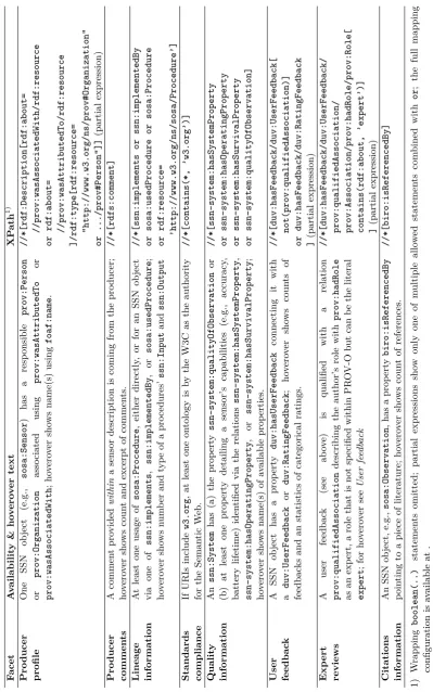
For example, for the facetProducer Commentsis set to available if a document contains

anrdfs:comment, because we can assume that such a comment stems from an entity involved

in the creation of the metadata record, for the facetCompliance with Standards, the mapping

checks if one of the used URIs containsw3.org and thereby denotes usage of a vocabulary

that underwent a development under the auspices of the Word Wide Web Consortium (W3C),

while for the mappingUser Feedbackan observation,sosa:Observation, must be connected

to a duv:UserFeedback based on the duv:hasUserFeedback property. However, not all mappings are so open respectively direct or simple and allow diﬀerent options. For example,

for the facet Producer Proﬁle an SSNO class such as sosa:Sensor can be connected to

a prov:Agent using either prov:wasAttributedTo or prov:wasAssociatedWith and the

4

https://www.w3.org/TR/vocab-ssn/#examples 5

(4)

respective PROV subclasses, and for the facet Lineage Information any of the relations ssn:implements,ssn:implementedBy, orsosa:usedProcedurecan connect a sensing system with its procedure documentation.

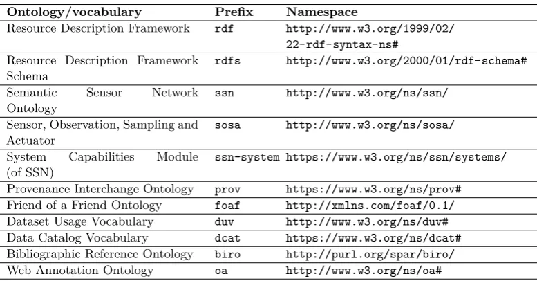
Table 1 summarises the result of the manual process and briefly explains the reasoning behind the chosen mapping. See Section 3.2 for the full details on the mapping and the technical realisation. The table shows the ontologies, classes, and properties we identified as suitable sources for the GEO label’s facets. The used ontologies and prefixes are listed in Table 2. Note that we did not add new alignments between the SSN and other ontologies, as that is beyond the scope of this work.

3 Serverless GEO label Generation

3.1 Serverless Computing

Serverless computing allows developers to deploy custom code in a shared infrastructure [2], whereby the application is maintained in a scalable way by a platform provider. The automated scaling enables both handling of large spikes of high demand and reducing costs when there is little or no demand. These properties make serverless computing a good ﬁt for the GEO label generation usage scenarios. The GEO label generation can be deployed to a serverless infrastructure quite easily, i.e., without a complex setup including multiple services or a database, because each generation of a label is a relatively small, stateless, atomic operation. The creation of a label externally only relies on the metadata sources for which a label is requested. However, depending on the usage scenario, requests for labels can be erratic and unpredictable. To demonstrate applicability of the prototype the evaluations were conducted within the free tier of the following service providers: Google

Cloud Run6_{(GCR) and Amazon Web Services (AWS) Lambda}7_{. A comparison of the costs,}

while relevant for potential operators, is out of scope for this work.

3.2 GEO label API Implementation

The GEO label API is implemented in two software projects, one in Java and one in PHP8.

In this work, the Java-based implementation is used because PHP is not supported by

the serverless computing providers and the PHP project is no longer maintained. The

rendering of the GEO label is based on an SVG template file. Labels are generated using the template file according to XPath expressions [7], which detect the presence of certain elements in a provided XML document. To use XPath, the RDF graph must be serialised in RDF/XML. Both implementations support a bespoke JSON-based configuration file format, which allows one to update the rules for transformations of metadata documents to labels without changes to the source code and to deploy these updates to GEO label API instances without updating the installation. To realise the conceptual mapping described above, we

created a new transformation ﬁle9_{. The ﬁle is activated when the implementation is provided}

as an RDF/XML document, i.e., if the XPathboolean(/*[local-name()='RDF'])testing

the document’s root element evaluates to true. Of note, the implementation of hoverover and drilldown features lies beyond the scope of the proof-of-concept implementation.

6

https://cloud.google.com/run/ 7 _{https://aws.amazon.com/lambda/}

8

https://geolabel.net/implementations.html 9 _{See transformation ﬁle source at}

(5)

T able 1 GEO lab el facets’ data sources in the Seman tic Sensor W eb F acet A v ailabilit y & ho v ero v er text XP ath 1) Pro ducer profile One SSN ob ject (e.g., sosa:Sensor ) has a resp onsible prov:Person or prov:Organization asso ciated using prov:wasAttributedTo or prov:wasAssociatedWith ; ho v ero v er sho ws name(s) using foaf:name . //*[rdf:Description[rdf:about= //prov:wasAssociatedWith/rdf:resource or rdf:about= _{//prov:wasAttributedTo/rdf:resource} ]/rdf:type[rdf:resource= "http://www.w3.org/ns/prov#Organization" or .../prov#Person"]] (partial expression) Pro ducer commen ts A commen t pro vided within a sensor description is coming from the pro ducer; ho v ero v er sho ws coun t and excerpt of commen ts. //*[rdfs:comment] Lineage information A t least one usage of sosa:Procedure , either directly , or for an SSN ob ject via one of ssn:implements , ssn:implementedBy , or sosa:usedProcedure ; ho v ero v er sho ws n um b er and typ e of a pro cedures’ ssn:Input and ssn:Output //*[ssn:implements or ssn:implementedBy or sosa:usedProcedure or sosa:Procedure or rdf:resource= ’http://www.w3.org/ns/sosa/Procedure’] Standards compliance If URIs include w3.org , at least one on tology is b y the W3C as the authorit y for the Seman tic W eb. //*[contains(*, ’w3.org’)] Qualit y information An ssn:System has (a) the prop ert y ssn-system:qualityOfObservation or (b) at least one prop ert y detailing a sensor’s capabilities (e.g., accuracy , battery lifetime) iden tified via the relations ssn-system:hasSystemProperty , ssn-system:hasOperatingProperty , or ssn-system:hasSurvivalProperty ; ho v ero v er sho ws name(s) of a v ailable prop erties. //*[ssn-system:hasSystemProperty or ssn-system:hasOperatingProperty or ssn-system:hasSurvivalProperty or ssn-system:qualityOfObservation] User feedbac k A SSN ob ject has a prop ert y duv:hasUserFeedback connecting it with a duv:UserFeedback or duv:RatingFeedback ; ho v ero v er sho ws coun ts of feedbac ks and an statistics of categorical ratings. //*[duv:hasFeedback/duv:UserFeedback[ not(prov:qualifiedAssociation)] or duv:hasFeedback/duv:RatingFeedback ] (partial expression) Exp ert reviews A user feedbac k (see ab o v e) is qualified with a relation prov:qualifiedAssociation describing the author’s role with prov:hadRole as an exp ert, a role that is not sp ecified within PR O V-O but can b e the literal expert ; for ho v ero v er see U ser fe edb ack //*[duv:hasFeedback/duv:UserFeedback/

prov:qualifiedAssociation/ prov:Association/prov:hadRole/prov:Role[ contains(rdf:about,

(6)

Table 2Used ontologies and vocabularies with their preﬁxes, and namespaces. Ontology/vocabulary Preﬁx Namespace

Resource Description Framework rdf http://www.w3.org/1999/02/

22-rdf-syntax-ns#

Resource Description Framework Schema

rdfs http://www.w3.org/2000/01/rdf-schema#

Semantic Sensor Network

Ontology

ssn http://www.w3.org/ns/ssn/

Sensor, Observation, Sampling and Actuator

sosa http://www.w3.org/ns/sosa/

System Capabilities Module

(of SSN)

ssn-system https://www.w3.org/ns/ssn/systems/

Provenance Interchange Ontology prov https://www.w3.org/ns/prov#

Friend of a Friend Ontology foaf http://xmlns.com/foaf/0.1/

Dataset Usage Vocabulary duv http://www.w3.org/ns/duv#

Data Catalog Vocabulary dcat https://www.w3.org/ns/dcat#

Bibliographic Reference Ontology biro http://purl.org/spar/biro/

Web Annotation Ontology oa http://www.w3.org/ns/oa#

Table 1 shows excerpts of the XPaths realising the conceptual mapping. The test data10

was created based on the example data for the SSN vocabulary11_{, which was converted}

to RDF/XML using two online converters for two varying serialisations into RDF/XML.

MyBluemix RDF Validator and Converter12_uses_rdf:resource_{attributes to deﬁne elements}

at one level (Listings 1), whereas Easy RDF Converter13 _{uses the class names as XML}

elements and nests the objects (2). These examples illustrate the reason for the complexity of the XPaths, which allow both options to serialise triples from an RDF graph in RDF/XML.

In GCR, the API can be deployed in a container, which allows one to run the whole

GEO label API with the existing Java Servlet14_. _{In AWS Lambda, however, the Java}

Servlet application cannot be run, so a subset of the GEO label API was implemented with

a bespoke request handling class15. This handler exposes the existing internal methods

for generating SVGs based on URLs to metadata documents provided by the API caller. Then, the API, i.e., the request parameters and allowed HTTP methods, are conﬁgured in the Amazon API Gateway. Figure 1 shows a GEO label rendered by the prototype implementation developed as part of this work.

3.3 Performance Evaluation

Two usage scenarios were evaluated with an Apache JMeter16 _{scripted test plan}17_{. For all}

API queries, the URL of the example RDF serialisation ﬁleMBC_all_factes_available_

ip68smartsensor.rdf hosted on GitHub is passed via the GET request query parameter

10

https://github.com/nuest/GEO-label-java/tree/master/testdata 11

https://www.w3.org/TR/vocab-ssn/#examples 12

http://rdfvalidator.mybluemix.net/ 13

http://www.easyrdf.org/converter 14

https://en.wikipedia.org/wiki/Java_servlet

15_{See code module}_lambda_:_{https://github.com/nuest/GEO-label-java/tree/master/lambda} 16

http://jmeter.apache.org/ 17_{JMeter test plan ﬁle}

(7)

Listing 1Observation, converted with MyBluemix RDF Validator and Converter.

< rdf : D e s c r i p t i o n

rdf : a b o u t =" h t t p :// e x a m p l e . org / d a t a / i c e C o r e / 1 2 # o b s e r v a t i o n " >

< s o s a : h a s S i m p l e R e s u l t

rdf : d a t a t y p e =" h t t p :// www . w3 . org / 2 0 0 1 / X M L S c h e m a # i n t e g e r " > 42

</ s o s a : h a s S i m p l e R e s u l t > < s o s a : o b s e r v e d P r o p e r t y

rdf : r e s o u r c e =" h t t p :// e x a m p l e . org / d a t a / i c e C o r e / 1 2 # CO2 "/ > < p r o v : w a s A s s o c i a t e d W i t h

rdf : r e s o u r c e =" h t t p :// e x a m p l e . org / d a t a / Org / e x a m p l e O r g "/ > < rdf : t y p e

rdf : r e s o u r c e =" h t t p :// www . w3 . org / ns / p r o v # A c t i v i t y "/ > < rdf : t y p e

rdf : r e s o u r c e =" h t t p :// www . w3 . org / ns / s o s a / O b s e r v a t i o n "/ > </ rdf : D e s c r i p t i o n >

rdf : a b o u t =" h t t p :// e x a m p l e . org / d a t a / Org / e x a m p l e O r g " >

< f o a f : name > E x a m p l e O r g a n i s a t i o n </ f o a f : name >

< rdf : t y p e rdf : r e s o u r c e =" h t t p :// www . w3 . org / ns / p r o v # O r g a n i z a t i o n "/ > < rdf : t y p e rdf : r e s o u r c e =" h t t p :// www . w3 . org / ns / p r o v # A g e n t "/ >

</ rdf : D e s c r i p t i o n >

metadatato the SVG-generating endpoint of the respective API deployments. The responses

are deemed successful if the HTTP status code is 200 (“OK”) and the content type is

image/svg+xml. The test plan results for all conducted tests are published in the software

repository18_{. An interactive app allows to inspect the plots of the results for all conducted}

tests, including ones not included in this article19_.

For both serverless computing providers, the default conﬁgurations were used for the evaluations. GCR allows users to conﬁgure the number of containers, the number of parallel requests handled by one container, and the required minimum response time. The GCR

deployment used zone europe-west1 with 256 Mebibyte working memory and 1 CPU, at

a concurrency setting of 80. AWS Lambda starts more instances of a Lambda function

as needed, limited by a conﬁgurable concurrency parameter (default value: 1000) for the

number of running functions in the used region eu-central-1. The working memory on

AWS is set to 1 Gibibyte with the default values for scaling20.

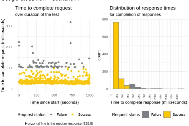
Scenario Asimulates a geospatial catalogue service with1000users whose browsing of

the catalogue user interface results in1 request per second per user. Figures 2 and 3 show

the response times during the test execution for GCR and AWS Lambda, respectively21_{. All}

sent requests have a non-failure status code (HTTP 200). The two diﬀerent colours in the

plots denote the requests that take less than (“Success”) or longer than (“Failure”)1second.

18_{JMeter test plan ﬁle}

GEO_Label_API.jmxand the result ﬁles are available online athttps://github. com/nuest/GEO-label-java/tree/master/misc/JMeterTests.

19

https://geolabel-ssno-paper.herokuapp.com/ 20

https://docs.aws.amazon.com/lambda/latest/dg/scaling.html 21_{Data loading and plot functions are based on code from the R package}

(8)

Figure 1 GEO label based on SSW sensor metadata, rendered by the GCR

deployment, with all eight facets fulﬁlled; source URL:

https://glbservice-nvrpuhxwyq- ew.a.run.app/glbservice/api/v1/svg?metadata=https://raw.githubusercontent.com/nuest/GEO-label-java/master/server/src/test/resources/ssno/ERC_all_factes_available_ip68smartsensor.rdf.

0 1000 2000 3000

0 250 500 750 1000

Time since start (seconds)

Time to complete request (milliseconds)

Request status Failure Success

over duration of the test

Time to complete request

Horizontal line is the median response (325.5)

0 200 400 600 800

0

250 500 750

1000 1250 1500 1750 2000 2250 2500 2750 3000

Time to complete response (milliseconds)

count

for completion of responses

Distribution of response times

Google Cloud Run − Scenario A

Figure 2 Plots of response time for GCR deployment under scenario A: elapsed time to complete requests (left); histrogram with distribution of response times (right); result data ﬁle:

(9)

Listing 2Observation, converted with Easy RDF Converter.

< s o s a : O b s e r v a t i o n

rdf : a b o u t =" h t t p :// e x a m p l e . org / d a t a / i c e C o r e / 1 2 # o b s e r v a t i o n " >

< rdf : t y p e rdf : r e s o u r c e =" h t t p :// www . w3 . org / ns / p r o v # A c t i v i t y "/ > < p r o v : w a s A s s o c i a t e d W i t h >

< p r o v : A g e n t

rdf : a b o u t =" h t t p :// e x a m p l e . org / d a t a / Org / e x a m p l e O r g " >

< rdf : t y p e

rdf : r e s o u r c e =" h t t p :// www . w3 . org / ns / p r o v # O r g a n i z a t i o n "/ > < f o a f : name > E x a m p l e O r g a n i z a t i o n </ f o a f : name >

</ p r o v : Agent >

</ p r o v : w a s A s s o c i a t e d W i t h > < s o s a : o b s e r v e d P r o p e r t y >

rdf : a b o u t =" h t t p :// e x a m p l e . org / d a t a / i c e C o r e / 1 2 # CO2 " > < ssn : i s P r o p e r t y O f

rdf : r e s o u r c e =" h t t p :// e x a m p l e . org / d a t a / i c e C o r e /12"/ > </ rdf : D e s c r i p t i o n >

</ s o s a : o b s e r v e d P r o p e r t y >

< s o s a : h a s S i m p l e R e s u l t

rdf : d a t a t y p e =" h t t p :// www . w3 . org / 2 0 0 1 / X M L S c h e m a # i n t e g e r " > 42

</ s o s a : O b s e r v a t i o n >

This threshold is used because interactions below one second were found to not interrupt a user’s train of thought and are therefore suitable for interactive use [20]. The mean times

to complete the request are414 seconds for GCR and943seconds for AWS Lambda.

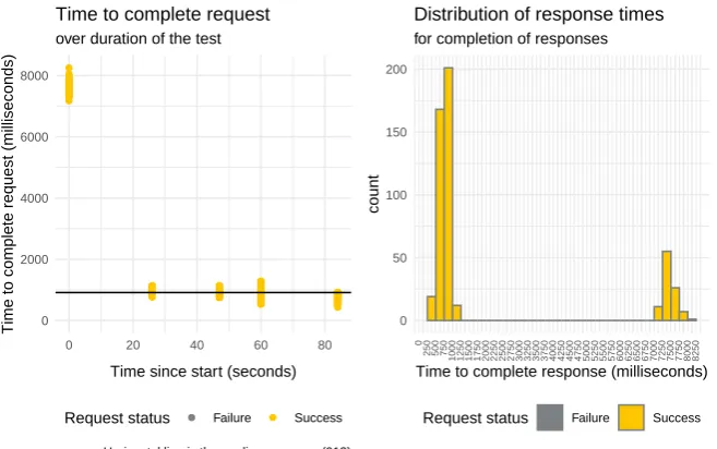
Scenario Btests the batch generation of labels where an operator of a sensor catalogue

wants to generate 100 labels at once. Here we measure the overall time for processing all

requests, and the operations were repeated5times. There is no threshold as in Scenario A.

For GCR, this led to failures due to the memory limit; but, the test was completed with a

memory of 1 Gibibyte and2 CPUs per container instance. The resulting data is shown in

Figure 4. GCR’s need for additional resources can be traced back to an overhead of the full Java Servlet, which the Lambda function handler, which is comparably more minimal, does

not suﬀer from. With the increased resources in GCR, the duration was up to 45seconds

for the ﬁrst run and decreased though to only about3 seconds for the ﬁfth repetition. For

AWS Lambda, the processing took about 8seconds on the ﬁrst run and dropped to around

1second in the second to ﬁfth repetitions, as shown in Figure 5.

A variant of the batch generation is a test scenario with 1000 parallel requests. This

scenario could not be completed by either platform with the maximum available hardware

conﬁgurations. The error messages (Connection resetandSSL handshake terminated)

hint that the services blocked the large number of parallel requests, such that users would

need more powerful (and more costly) deployments. Reducing the number of parallel

requests eventually led to successful scenario executions at 600 requests in 51 seconds for

GCR and300requests in9seconds for AWS Lambda (see data ﬁlesGCR_Scenario_4_2_V3

(10)

0 2000 4000 6000 8000

0 250 500 750 1000

Horizontal line is the median response (1028)

0 200 400 600

0

250 500 750

1000 1250 1500 1750 2000 2250 2500 2750 3000 3250 3500 3750 4000 4250 4500 4750 5000 5250 5500 5750 6000 6250 6500 6750 7000 7250 7500 7750 8000

count

AWS − Scenario A

Figure 3 Plots of response time for AWS deployment in scenario A: elapsed time to complete requests (left); histrogram with distribution of response times (right); result data ﬁle:

AWS_Scenario_2_V1.

0 10000 20000 30000 40000

0 50 100 150

0 50 100

0

2000 4000 6000 8000

10000 12000 14000 16000 18000 20000 22000 24000 26000 28000 30000 32000 34000 36000 38000 40000 42000 44000

count

GCR − Scenario B

(11)

0 2000 4000 6000 8000

0 20 40 60 80

0 50 100 150 200

0

250 500 750

1000 1250 1500 1750 2000 2250 2500 2750 3000 3250 3500 3750 4000 4250 4500 4750 5000 5250 5500 5750 6000 6250 6500 6750 7000 7250 7500 7750 8000 8250

count

AWS − Scenario B

Figure 5 Plots of response time for AWS deployment in scenario A: elapsed time to complete requests (left); histrogram with distribution of response times (right); result data ﬁle:

AWS_Scenario_3_V2.

4 Discussion

Themappingof GEO label facets to properties in the Semantic Sensor Web was an iterative process. While we were able to ﬁnd data sources for all GEO label facets, the mapping is limited by the availability of realistic SSW datasets. First, the variability of real-world data may not be adequately captured. Second, and the nature of the mapping does not capture cases where concepts between the GEO label’s facets do not unambiguously match concepts behind SSW elements. Compared to the centrally managed data sources and industry-driven OGC standards of the original GEO label, we ﬁnd no need to make distinctions between metadata given by providers and by third-parties, e.g., commenting servers. However, such multi-stakeholder perspectives could mitigate shortcomings in the creation process of the GEO label mapping for SSW. More real-world metadata could improve the scope of the facet data sources, e.g., by deriving from common practices if a comment is actually about a relevant part of a sensor’s properties, and not about some less relevant part of the RDF

graph. The taken iterative, example-based approach could also be contrasted with the

initial creation of an ontology for the GEO label facets and then aligning the GEO label ontology with existing (SSW) ontologies. The alignment-based approach could also improve the scalability of the mapping for a larger variety of uses cases and SSW datasets.

Concerning the mapping’simplementation, we found that a document-based approach

(12)

into account relationships between linked resources by, for example, measuring the distance between connected resources in a graph. The GEO label’s option to have “half-filled” facets, which denotes availability of information at a higher level, could expose such more complex scenarios. Most critically, the presented approach is limited by the design process starting only from the current GEO label facets. That is why specific discovery challenges of the SSW may not be adequately addressed. While the label itself may be interactive, the majority of information behind the label is seen as rather static. This may partly be attributed to the GEO label’s origin in GEO, with more traditional roles of provider and user. The SSW’s potentially very dynamic nature, for examples live data streams, and flexible distributed architecture, in which anybody can create and publish new ontologies and datasets, may require additional facets or a more sophisticated presentation of sources and currentness of the data behind a label.

Theevaluationresults of Scenario A show show no discernible cold start eﬀect, as one might have expected, where resources need to be activated for the ﬁrst request or additional

resources are added over time. Only few requests take over1second to complete and only

relatively few outliers exists on the same order of magnitude. For AWS Lambda, both

mean and median of elapsed time to complete a request are close to1 second. For GCR,

the elapsed time is well below 0.5 seconds. These results imply that the serverless label

generation is suitable for interactive use, with slight advantages of GCR which has overall shorter durations. A limitation for this scenario is that only the generation of the label is tested, whereas for users additional time would be taken up by the client-side rendering of the images. The eﬀects of dropping durations for batch processing in Scenario B were likely achieved by a combination of autoscaling in the underlying platforms and the built-in caching of the GEO label API Java Servlet. Especially on AWS Lambda, the drop after the ﬁrst iteration is considerable, even tough no internal caching mechanism exists.

(13)

5 Conclusions

In this study, we transferred the goal of the GEO label, which is to improve data discovery by providing a visual overview of available information in machine-readable metadata, to the Semantic Sensor Web. While we were able to ﬁnd data sources for all GEO label facets using a document-centric approach, the mapping is limited by available datasets and does not leverage the potential of using reasoning in the SSW. Ideally, the creation of a more sustainable mapping and potentially even adaptation of GEO label facets in the future is based on a larger body of public sensor metadata in SSNO format, on a consultation of multiple stakeholders, and on a complementary perspective derived from the SSW’s discovery challenges.

We found that the serverless platforms proved suitable for realistic test scenarios, though, naturally, the used free tiers have limits. It became also clear that the different cost models and configurations make serverless solutions difficult to compare. Future evaluations may utilise a strictly cost-based comparison of scenarios with resources tuned to deliver similar performance in the user-facing API.

Finally, the usefulness of the GEO label remains to be demonstrated in broad deployments with many users and extensive user studies. With the practical solutions for label generation introduced in this work, the actual spreading of labels will require leading organisations to add and maintain labels on their widely used geospatial catalogues. In the meantime, a bottom-up approach with client-side label integration [23] could provide the beneﬁts of GEO labels to interested users, and the GEO label can be examined in relation to recent developments on scientiﬁc data publication such as the FAIR Guiding Principles [26].

References

1 Grigori Babitski, Simon Bergweiler, Jörg Hoﬀmann, Daniel Schön, Christoph Stasch, and

Alexander C. Walkowski. Ontology-Based Integration of Sensor Web Services in Disaster

Management. In Krzysztof Janowicz, Martin Raubal, and Sergei Levashkin, editors,

GeoSpatial Semantics, Lecture Notes in Computer Science, pages 103–121, Berlin, Heidelberg,

2009. Springer. doi:10.1007/978-3-642-10436-7_7.

2 Ioana Baldini, Paul Castro, Kerry Chang, Perry Cheng, Stephen Fink, Vatche Ishakian,

Nick Mitchell, Vinod Muthusamy, Rodric Rabbah, Aleksander Slominski, and Philippe Suter. Serverless Computing: Current Trends and Open Problems. In Sanjay Chaudhary, Gaurav

Somani, and Rajkumar Buyya, editors,Research Advances in Cloud Computing, pages 1–20.

Springer, Singapore, 2017. doi:10.1007/978-981-10-5026-8_1.

3 Mike Botts, George Percivall, Carl Reed, and John Davidson. OGC®sensor web enablement:

Overview and high level architecture. InGeoSensor Networks, pages 175–190. Springer Berlin

Heidelberg, 2008. doi:10.1007/978-3-540-79996-2_10.

4 Dan Brickley and Libby Miller. FOAF Vocabulary Speciﬁcation. Technical report, January

2014. URL:http://xmlns.com/foaf/spec/.

5 Jean-Paul Calbimonte, Hoyoung Jeung, Oscar Corcho, and Karl Aberer. Semantic sensor

data search in a large-scale federated sensor network. InProceedings of the 4th international workshop on semantic sensor networks, volume 839 of CEUR Workshop Proceedings, pages

23–38, Bonn, Germany, 2011. URL:http://ceur-ws.org/Vol-839/calbimonte.pdf.

6 Eliot J. Christian. GEOSS Architecture Principles and the GEOSS Clearinghouse. IEEE

Systems Journal, 2(3):333–337, September 2008. Conference Name: IEEE Systems Journal.

doi:10.1109/JSYST.2008.925977.

7 J. Clark and S. DeRose. XML Path Language (XPath), Version 1.0. W3C Recommendation,

(14)

8 Erik Dahlström, Patrick Dengler, Anthony Grasso, Chris Lilley, Cameron McCormack, Doug Schepers, and Jonathan Watt. Scalable Vector Graphics (SVG) 1.1 (Second Edition). W3C

Recommendation, 2011. URL:http://www.w3.org/TR/SVG/.

9 Angelo Di Iorio, Andrea Nuzzolese, Silvio Peroni, David Shotton, and Fabio Vitali. Describing bibliographic references in RDF. In Alexander Garc{\’i}a Castro, Christoph Lange, Phillip

Lord, and Robert Stevens, editors,4\textsuperscript{th} Workshop on Semantic Publishing

(SePublica 2014), volume 1155 ofCEUR Workshop Proceedings, Anissaras, Greece, May 2014. URL:http://ceur-ws.org/Vol-1155/paper-05.pdf.

10 Bernadette Farias Lóscio, Eric G. Stephan, and Sumit Purohit. Data on the Web Best

Practices: Dataset Usage Vocabulary. Technical report, 2016. Library Catalog: www.w3.org. URL:https://www.w3.org/TR/vocab-duv/.

11 Anika Graupner. Ein Metadatenlabel für das semantische Sensorweb. April 2020. doi:

10.31237/osf.io/fs48a.

12 Armin Haller, Krzysztof Janowicz, Simon J. D. Cox, Maxime Lefrançois, Kerry Taylor, Danh

Le Phuoc, Joshua Lieberman, Raúl García-Castro, Rob Atkinson, and Claus Stadler. The modular SSN ontology: A joint W3C and OGC standard specifying the semantics of sensors,

observations, sampling, and actuation. Semantic Web, 10(1):9–32, January 2019. doi:10.

3233/SW-180320.

13 Steve Harris and Andy Seaborne. SPARQL 1.1 Query Language. W3C Recommendation,

March 2013. URL:https://www.w3.org/TR/sparql11-query/.

14 Krzysztof Janowicz, Sven Schade, Arne Bröring, Carsten KeSSler, Patrick Maué, and

Christoph Stasch. Semantic Enablement for Spatial Data Infrastructures. Transactions in

GIS, 14(2):111–129, 2010. doi:10.1111/j.1467-9671.2010.01186.x.

15 Hoyoung Jeung, Soﬁane Sarni, Ioannis Paparrizos, Saket Sathe, Karl Aberer, Nicholas

Dawes, Thanasis G. Papaioannou, and Michael Lehning. Eﬀective Metadata Management

in Federated Sensor Networks. In2010 IEEE International Conference on Sensor Networks,

Ubiquitous, and Trustworthy Computing, pages 107–114, June 2010.doi:10.1109/SUTC.2010. 29.

16 Simon Jirka, Arne Bröring, and Christoph Stasch. Discovery Mechanisms for the Sensor Web.

Sensors, 9(4):2661–2681, April 2009. doi:10.3390/s90402661.

17 Timothy Lebo, Satya Sahoo, and Deborah McGuinness. PROV-O: The PROV Ontology.

Technical report, April 2013. Publisher: W3C. URL:https://www.w3.org/TR/prov-o/.

18 Victoria Lush. Visualisation of quality information for geospatial and

remote sensing data: providing the GIS community with the decision support tools for geospatial dataset quality evaluation. PhD thesis, Aston

University, 2015. URL: https://research.aston.ac.uk/en/studentTheses/

visualisation-of-quality-information-for-geospatial-and-remote-se.

19 Victoria Lush, Lucy Bastin, and Jo Lumsden. Developing a geo label: providing the gis

community with quality metadata visualisation tools. Proceedings of the 21st GIS Research UK (GISRUK 3013), Liverpool, UK, pages 3–5, 2013. URL: https://www.geos.ed.ac.uk/ ~gisteac/proceedingsonline/GISRUK2013/gisruk2013_submission_44.pdf.

20 Jakob Nielsen. Response Times: The 3 Important Limits, January 1993. URL: https:

//www.nngroup.com/articles/response-times-3-important-limits/.

21 Jacqueline Nolis. loadtest: HTTP load testing directly from R, 2020. R package version 0.1.2. URL:https://github.com/tmobile/loadtest.

22 Daniel Nüst and Anika Graupner. nuest/GEO-label-java: Release 0.3.0, February 2020.doi:

10.5281/zenodo.3673870.

23 Daniel Nüst, Lukas Lohoﬀ, Lasse Einfeldt, Nimrod Gavish, Marlena Götza, Shahzeib Tariq

Jaswal, Salman Khalid, Laura Meierkort, Matthias Mohr, Clara Rendel, and Antonia van Eek. Guerrilla Badges for Reproducible Geospatial Data Science. AGILE Short Papers, Limassol,

(15)

24 Daniel Nüst and Victoria Lush. A GEO label for the Sensor Web. AGILE Short Papers,

Lisbon, Portugal, 2015. AGILE. doi:10.31223/osf.io/ka38z.

25 Amit Sheth, Cory Henson, and Satya S. Sahoo. Semantic Sensor Web. IEEE Internet

Computing, 12(4):78–83, July 2008. doi:10.1109/MIC.2008.87.

26 Mark D. Wilkinson, Michel Dumontier, IJsbrand Jan Aalbersberg, Gabrielle Appleton, Myles