The development of a 10 mK refrigeration system for space

(1)

The Development of a 10 mK

Refrigeration System for Space

Michael Robert Ernes

Mullard Space Science Laboratory Department o f Space and Climate Physics

University College London

A thesis submitted in accordance with the regulations for the degree o f Doctor o f Philosophy in the University o f London

(2)

ProQuest Number: 10013939

INFORMATION TO ALL USERS

The quality of this reproduction is dependent upon the quality of the copy submitted.

In the unlikely event that the author did not send a complete manuscript and there are missing pages, these will be noted. Also, if material had to be removed,

a note will indicate the deletion.

uest.

ProQuest 10013939

Published by ProQuest LLC(2016). Copyright of the Dissertation is held by the Author.

This work is protected against unauthorized copying under Title 17, United States Code. Microform Edition © ProQuest LLC.

ProQuest LLC

789 East Eisenhower Parkway P.O. Box 1346

(3)

Abstract

Detectors already require cooling to millikelvin temperatures in space to maximize energy resolution so that more distant sources o f radiation can be identified. The lowest temperature that has been achieved in orbit so far is 302 mK on the infrared telescope for space (IRTS) in 1995. The Japanese ASTRO-E satellite launched unsuccessfully in February 2000 was to achieve 65 mK. Future instruments such as ESA ’s x-ray evolving universe spectrometer (XEUS) will require cooling to 30 mK and below.

This thesis presents the design o f a cryogenic cooling system that will surpass the needs o f XEUS and encourage the development o f a new generation o f very low temperature, high-resolution detectors for space.

With a single mechanical cooler maintaining thermal shield temperatures o f 150 K, 20 K and 4 K, the adiabatic demagnetization refi-igerator (ADR) proposed cools from a bath temperature o f 4 K to 10 mK. The maximum amount o f time for which the ADR can maintain this temperature is around 145 hours with no cooling power on the detector stage. This value falls as the cooling power increases, with a heat lift from the detector stage o f 100 nW possible for 30.6 hours’ continuous operation. A recycle time o f around two hours is required between successive cycles.

(4)

List of Figures

Figure Figure Figure Figure Figure Figure Figure Figure Figure Figure Figure Figure Figure Figure Figure Figure Figure Figure Figure Figure Figure Figure Figure

-1 : Axial acceleration profile for Ariane 4 ... 24

-2: Components of radiation incident upon spacecraft...27

-3: View factor geometry between planet and satellite...30

-4: Albedo radiation incident on satellite... 32

-5: ISO spacecraft...36

-6: Lower and lower temperatures required for space instruments...37

-7: Spacecraft refi'igeration systems... 40

-8: Carbon - Carbon (C-C) radiator... 42

-9: Worst case passive radiator performance... 45

-10: Spacecraft orbiting the Earth with constant attitude...46

-11: Optimum attitude for constant attitude spacecraft...46

-12: View factor and visibility factor as functions of orbital position, 0 ... 47

-13: Cooling power vs. orbital angle, 0, for various radiator temperatures, T ... 48

-14: Mean cooling power over orbit as a function of radiator temperature, T ... 48

-15: Components of radiation as a function of 6 for 200 K radiator...50

-16: Bimetallic radiation fins...52

-17: Temperatures typically achievable with various cryogenic technologies... 54

-18: Equilibrium between helium liquid and vapour... 55

-19: Flight cryostat for COBE...58

-20: A helium adsorption cooler for space... 60

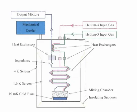
-21: Schematic of helium-3/helium-4 dilution refi*igerator for space... 63

-22: Ideal Carnot refrigeration cycle set-up... 66

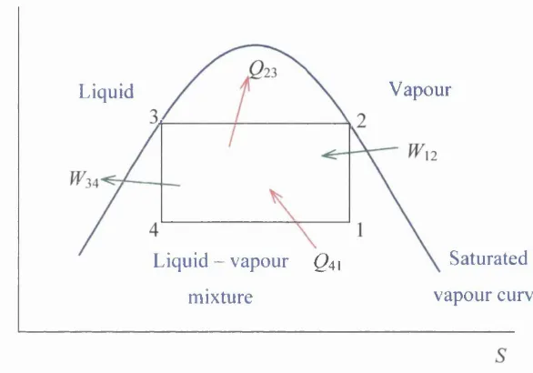
-23: T-S diagram for Carnot reftigeration cycle... 67

Figure 1-24: Carnot cycle COP for all Tc/Th...69

Figure 1-25: Carnot cycle COP for low Tc/Th... 69

Figure 1-26: Ball Aerospace Stirling cycle cooler...71

Figure 1-27: Schematic o f Stirling refiigeration c y c le ... 72

Figure 1-28: p-v diagram for Stirling refrigeration c y c le ...73

Figure 1-29: T-S diagram for Stirling refrigeration cycle... 73

(11)

List o f Figures

Figure 1-31 : Various pulse tube refrigerator heads... 76

Figure 1-32: AIRS pulse tube refrigerator for space... 78

Figure 1-33: Principle of isentropic cooling...80

Figure 1-34: Principle of adiabatic demagnetization refrigeration... 81

Figure 1-35: T-S diagram for magnetic cooling (for comparison with Figure 1-23)... 81

Figure 2-1 : Components of an A DR...88

Figure 2-2: DGG crystal for space ADR...92

Figure 2-3: Superconducting magnet for laboratory A DR... 93

Figure 2-4: Thermal shields around 10 mK A D R ... 97

Figure 2-5: Typical strap shape...98

Figure 2-6: Possible strap attachment regime... 99

Figure 2-7: Suspension strap geometry (third angle projection)... 100

Figure 2-8: Single-stage ADR layout... 101

Figure 2-9: Laboratory single-stage ADR... 102

Figure 2-10: Two-stage ADR layout... 103

Figure 2-11: Solid model of laboratory dADR...105

Figure 2-12: Double ADR (dADR) layout...106

Figure 3-1 : Position vectors of suspension straps...116

Figure 3-2: The effect of variable stiffiiess on strap tension... 122

Figure 3-3: Geometry of straps connecting adjacent enclosures... 130

Figure 3-4: Rotation of a mass subjected to sinusoidal vibrations... 134

Figure 3-5: Single-mass model for vibrations analysis...136

Figure 3-6: Stresses in suspension straps as functions of tim e... 140

Figure 3-7: Stresses due to simultaneous excitations in x, y and z-directions...143

Figure 3-8: Five-mass analytical model for prediction of launch vibrations... 144

Figure 3-9: Physical significance of rigid enclosure approximation... 149

Figure 3-10: Displacement of rod element... 150

Figure 3-11: First normal mode of shell vibration...158

Figure 3-12: Schematic of shell showing in-phase displacements... 159

Figure 3-13: Second normal mode of shell vibration...159

Figure 3-14: Schematic of shell showing anti-phase displacements... 160

Figure 3-15: Worst case geometry with flexible enclosures... 161

Figure 3-16: Difference between midpoint displacement and end displacement...162

(12)

List o f Figures____________________________________________________________ 10

Figure 3-18: Stress profile along shell for excitation frequency of 2000 H z...165

Figure 3-19: Calculation of gravity-force induced stress along the shell... 166

Figure 3-20: Variation of gravity-force induced stress along shell... 166

Figure 3-21: Vertical straps for calculation of shield stress due to strap tensions...168

Figure 3-22: Displacements of bodies under y-direction (vertical) excitation...172

Figure 3-23: Initial response of masses to sinusoidal excitations... 172

Figure 3-24: Velocities of masses under sinusoidal y-direction excitation...173

Figure 3-25: Initial velocities of masses subjected to vertical excitations... 174

Figure 3-26: Stresses in five-mass system under vertical sinusoidal excitation...175

Figure 3-27: Forcing acceleration to failure under y-direction (vertical) excitations...177

Figure 3-28: Near resonance response of system...178

Figure 3-29: Peak stresses with damping constant reduced by factor often... 180

Figure 3-30: Comparison of normal damping and low damping peak stresses...181

Figure 3-31 : Forcing acceleration to failure with 1/10**’ damping constant... 182

Figure 3-32: Forcing acceleration to failure at natural frequency with 1/10**’ damping 183 Figure 3-33: Peak stresses under x-z plane sinusoidal excitation... 184

Figure 3-34: Forcing acceleration to failure under x-z plane excitations... 186

Figure 3-35: x-z plane forcing acceleration to failure near resonance... 186

Figure 3-36: x-z plane forcing acceleration to failure with 1/10**’ damping...187

Figure 3-37: x-z plane acceleration to failure with 1/10**’ damping near resonance...188

Figure 4-1: Dimensions of aluminium enclosures...197

Figure 4-2: Heat flow between concentric enclosures...199

Figure 4-3: Calculation of strap lengths...202

Figure 4-4: Heat flow in current leads...205

Figure 4-5: Temperature distribution along 150 K - 300 K current leads...211

Figure 4-6: Optimum current lead diameter for aluminium wires...212

Figure 4-7: Heat load components on 4 K enclosure... 215

Figure 4-10: Hold time for 10 mK dADR as a function of detector heat load...220

Figure 4-11 : Effect of changing cord diameter on hold time... 221

Figure 4-12: Hold time as a function of cord diameter for low input powers... 222

Figure 4-13: Hold time as a function of heat load on DGG...223

Figure 4-14: Hold time as a function of heat load on CMN...223

(13)

List o f Figures____________________________________________________________ H

Figure 5-1 : The effect of MLI on radiative heat transfer... 233

Figure 5-2: Mechanical model with 65 K shield... 236

Figure 5-3: Double ADR layout for suspension cord optimization...244

Figure 5-4: Clearance required for attaching cords... 247

Figure 5-5: Hold times for an optimized dADR with no heat load on detectors... 250

Figure 5-6: The effect of changing cord length with 1 pW heat load on detector stage 250 Figure 5-7: The effect of changing cord lengths with 0 W on CMN, 20 pW on DGG 251 Figure 5-8: Hold time vs. cord length with 200 nW on CMN, 20 pW on DGG... 252

Figure 6-1: Schematic of dADR former...257

Figure 6-2: Field contribution due to each current loop... 259

Figure 6-3: Cross-section through magnet former showing distance between wires... 261

Figure 6-4: Alternative orientation for nearest wires... 262

Figure 6-5: Mesh of nodes for description of magnetic field... 264

Figure 6-6: Grouping of wire loops to reduce computations... 265

Figure 6-7: Definition of turns density...266

Figure 6-8: Optimum geometry of main magnet winding... 268

Figure 6-9: Field modulus as a function of axial position... 270

Figure 6-10: 3-D plot of single solenoid’s field occupied by CM N ...271

Figure 6-11 : Variation of field components with radius (z = 90 mm)...272

Figure 6-12: Variation of field components with axial position (r = 44 mm)...273

Figure 6-13: Arrangement of main solenoid with cancellation coils...274

Figure 6-14: Fields due to left cancellation coil (r = 44 mm)... 275

Figure 6-15: Fields due to right cancellation coil (r = 44 mm)... 275

Figure 6-16: Field strength vs. axial position with cancellation coils (r = 44 mm)... 276

Figure 6-17: Field components vs. radius with cancellation coils (z = 90 mm)... 277

Figure 6-18: Effect of cancellation coils on field modulus vs. axial position... 278

Figure 6-19: Schematic of magnet former and windings... 279

Figure 6-20: Plane strain conditions for former and windings... 280

Figure 6-21 : Axial force on each loop of w ire... 284

Figure 6-22: Forces within the windings due to radial component of field...285

Figure 6-23: Equal and opposite forces compressing the windings...286

Figure 6-24: Stresses at midpoint (z = 50 mm) of main solenoid... 291

Figure 6-25: Radial displacement as a function of radius (z = 50 mm)...291

Figure 6-26: Eddy currents flowing in elemental annulus... 296

(14)

List o f Figures____________________________________________________________ 12

Figure 6-28: Magnet former with m slots of depth d... 303

Figure 6-29: Eddy current heating as a function of slot depth for copper former... 308

Figure 6-30: Eddy current heating as a function of number of slots for copper... 309

Figure 6-31 : Eddy current heating as a function of slot depth for aluminium former 310 Figure 6-32: Eddy current heating as a function of number of slots for aluminium 311 Figure 6-33: Hybrid magnet former layout...314

Figure 6-34: Section through hybrid magnet former... 316

Figure 6-35: Axial stresses in hybrid former... 321

Figure 6-36: Stresses for hybrid former with 2 mm copper conductor layer... 322

Figure 6-37: Stresses for hybrid former with 0.5 mm aluminium conductor layer 323 Figure 6-38: Hybrid magnet former design for eddy current analysis...326

Figure 6-39: Design of formers for experimental testing of cooling performance... 329

Figure 6-40: Cooling curve for solid copper magnet former... 330

Figure 6-41: Cooling performances of simple formers... 331

(15)

13

List of Tables

Table 1-1: Sources of structural loading... 23

Table 1-2: Temperature tolerances of typical spacecraft components... 26

Table 1-3: Average planetary albedo, a... 31

Table 1-4: Radiator performance at various temperatures, T ... 49

Table 2-1 : Important properties of some paramagnetic materials...90

Table 2-2: Comparison between types of ADR... 107

Table 2-3: Summary of ADR components... 108

Table 3-1 : Sinusoidal vibration qualification levels... 112

Table 3-2: Random vibration qualification levels... 113

Table 3-3: Physical parameters for single-mass vibration analysis...115

Table 3-4: Comparison of Model 1 and Model 2 results... 141

Table 3-5: The effect of combined excitation in more than one direction... 142

Table 3-6: Dimensions of suspension straps... 147

Table 3-7: Masses of system components... 148

Table 3-8: Natural frequencies for y-direction excitation...176

Table 3-9: Natural frequencies for x-z plane (lateral) excitations...184

Table 3-10: Natural frequencies for vibrations in x, y and z-directions...189

Table 3-11 : Results of y-direction random vibration analysis...190

Table 3-12: Results of x-z plane random vibrations analysis...191

Table 3-13: Comparison of sinusoidal results with launch qualification levels... 192

Table 3-14: Safety factors for sinusoidal excitation... 193

Table 3-15: Salient forcing accelerations to failure... 195

Table 4-1 : Net radiated heat load upon each enclosure...201

Table 4-2: Suspension strap material choices... 203

Table 4-3: Conducted heat loads on each enclosure...204

Table 4-4: Minimum heat loads along current leads...210

(16)

List o f Tables_____________________________________________________________ 14

Table 4-6: Cryocooler heat lift capability... 214

Table 4-7: Default parameters for thermal modelling of ADR... 218

Table 4-8: Hold time as a function of final CMN temperature... 225

Table 4-9: Summary of ADR performance...226

Table 5-1: Properties of possible thermal shield materials... 231

Table 5-2: Safety factors and masses for various shield thicknesses... 232

Table 5-3: Description of suspension system with 65 K shield... 237

Table 5-4: Description of masses in six-mass system...238

Table 5-5: Natural frequencies of six-mass system...238

Table 5-6: Summary of mechanical performance with 65 K enclosure... 239

Table 5-7: Salient forcing accelerations to failure...239

Table 5-8: Heat loads with 65 K shield... 240

Table 5-9: Heat loads without 65 K shield... 241

Table 5-10: Summary of hold times with optimized geometries... 254

Table 6-1 : Maximum values of k for different wires...262

Table 6-2: Summary of maximum stresses in magnet (MPa)... 292

Table 6-3: Summary of maximum stresses in magnet with 20 mm former (MPa)...292

Table 6-4: Stresses in magnet with 5 mm thick aluminium 6082 former (MPa)...294

Table 6-5: Comparison of eddy current heating with aluminium and copper formers...299

Table 6-6: Summary of effect of slotting copper former...309

Table 6-7: Summary of effect of slotting aluminium 6082 former... 311

Table 6-8: Stresses (MPa) for hybrid former with 2 mm copper conductor... 323

Table 6-9: Stresses (MPa) for hybrid former with 0.5 mm aluminium conductor...324

Table 6-10: Summary of magnet former performances...327

(17)

15

List of Abbreviations

A BRIXA S A BRoadband Imaging X-ray All-sky Survey A D R Adiabatic Demagnetization Refrigerator A IR S Atmospheric InfraRed Sounder

A ST R O -E Fifth Japanese x-ray astronomy mission C C D Charge Coupled Device

C E A Commissariat a l’Energie Atomique (French atomic energy authority) C F R P Carbon-Fibre Reinforced Plastic

C IS Cryogenic Imaging Spectrometer C M N Cerium Magnesium Nitrate C O B E COsmic Background Explorer

C O BR A S COsmic Background Radiation Anisotropy Satellite C O P Coefficient O f Performance

C PA Chromic Potassium Alum

dA D R double Adiabatic Demagnetization Refrigerator D G G Dysprosium Gallium Garnet

e.m.f. electromotive force

E M I ElectroMagnetic Interference E O S Earth Observing System ESA European Space Agency F IR P Far InfraRed Photometer G G G Gadolinium Gallium Garnet

G SFC Goddard Space Flight Center (NASA) IR A S InfraRed Astronomical Satellite IR T S InfraRed Telescope for Space

ISAM S Infrared Stratospheric And Mesospheric Sounder ISO Infrared Space Observatory

(18)

List o f Abbreviations 16

J P L Jet Propulsion Laboratory (NASA) J T Joule-Thomson

LE O Low Earth Orbit M L I Multi-Layer Insulation M M S Matra-Marconi Space M S Maximum Stress

M SSL Mullard Space Science Laboratory

NASA National Aeronautics and Space Administration O PT R Orifice Pulse Tube Refrigerator

PL A N C K Formerly COBRAS/SAMBA - renamed in honour o f Max Planck PSD Power Spectral Density

RA L Rutherford Appleton Laboratories r.m .s. root mean square

SAM BA SAtellite for Measurement o f Background Anisotropies SET Service des Basses Températures (Grenoble, France) SH O O T Superfluid Helium On Orbit Transfer

SR Stirling cycle Refrigerator

S T J Superconducting Tunnel Junction

ST J-C Superconducting Tunnel Junction Camera TES Transition Edge Sensor

W EI Wide Field Imager

XEUS X-ray Evolving Universe Spectroscopy mission XRS X-Ray Spectrometer

Y BCO Yttrium Barium Copper Oxide

(19)

17

A cknowledgements

My thanks go to my supervisor, Ian Hepburn, and the rest o f the team at MSSL. In particular, I would like to thank W ilf Oliver for his advice on vibrations modelling and Eric Crofts for his help with the hybrid magnet former design.

I’ve appreciated Graham Hardy’s efforts to entertain me with Quake III, and the football crew ’s unswerving commitment, with countless entertaining episodes on the rabbit-warren.

(20)

18

Overview of Thesis

This thesis presents the design o f a long-life refrigeration system capable o f cooling to 10 mK in space.

The first chapter introduces the field o f space cryogenics, explaining why cooling to 10 mK in space is desirable and outlining the current technologies that can provide such low temperatures. The harsh space environment is described, including the thermal environment in which the spacecraft must operate and the mechanical stresses to which spacecraft are subjected before, during and after launch. It is shown that the technology best suited to achieving a temperature o f 10 mK in space is an adiabatic demagnetization refrigerator (ADR), pre-cooled by passive radiators and a mechanical cooler.

The components o f a 10 mK ADR are described in Chapter 2. In particular, the importance o f the paramagnetic refrigerant, the superconducting magnet and the suspension straps is stressed.

(21)

Overview o f Thesis________________________________________________________ 19

Chapter 5 presents an optimization o f both the system o f thermal shields that reduces the radiative heat load on the coldest parts o f the system and the geometry o f the ADR. The latter is particularly important if paramagnetic materials and suspension straps compete for a limited amount o f space within the magnet bore.

The design o f the superconducting magnet is the subject o f Chapter 6. The magnetic field profile, the stresses in the magnet and the eddy current heating in the former are analysed for a space ADR. A ‘hybrid’ aluminium alloy/composite magnet former is presented, which has low mass and good thermal and mechanical properties.

With the main features o f the 10 mK refrigerator established, the conclusions o f the thesis are presented in Chapter 7. This includes a summary o f what has been achieved, and suggestions for further work.

Finally, references are listed in Chapter 8.

(22)

20

1 Introduction to Space

Cryogenics

Overview o f Chavter 1

In this chapter, we discuss what ‘space cryogenics’ means, why it is useful and what different cryogenic technologies exist.

First, Section 1.1 answers the question ‘what is space cryogenics’. Section 1.2 describes the space environment and contrasts the temperatures available with cryogenic cooling with the ambient temperature in space. This is followed in Section

1.3 with a discussion o f what space cryogenics has to offer, and Section 1.3.1 outlines the need for 10 mK refrigeration in space.

Section 1.4 moves on to the more practical question o f how cryogenic temperatures are achieved in space and outlines the benefits o f the various technologies available.

(23)

Chapter 1 Introduction to Space Cryogenics_________________________________21

1.1 What is space cryogenics?

The word cryogenics is derived from the Greek word ‘kruos’, which means ‘frost’ or ‘icy cold’. According to the Oxford English Dictionary, cryogenics is therefore “the branch o f physics and technology that deals with the production o f very low temperatures and their effects” \ ‘Very low temperatures’ means different things to different people, but it seems reasonable to assume that the temperatures o f all ‘cryogens’ must be cryogenic. The cheapest and most widely used cryogen is liquid nitrogen, which makes accessible temperatures down to its boiling point o f 77 K (- 196 °C). Probably the most common concept o f a cryogenic temperature is therefore a temperature around or below the boiling point o f liquid nitrogen at 77 K.

In fact, this thesis describes a refrigeration system capable o f cooling to 10 mK (- 273.14 °C), one hundredth o f a degree Celsius above absolute zero (-273.15 °C). In the context o f this thesis, therefore, a ‘very low temperature’ usually refers to a temperature below 1 K (-272.15 °C). Nevertheless, ‘cryogenic’ will generally be used to describe temperatures below around 77 K.

(24)

Chapter 1 Introduction to Space Cryogenics__________________________________22

1.2 The space environment

In addition to the obvious difficulty in providing maintenance in space, there are three important differences between a space environment and that o f a laboratory on Earth.

Firstly, there is no atmosphere in space. Our atmosphere traps much o f the infrared radiation that is emitted by the surface o f the planet by the greenhouse effect. This means that the mean temperature on the surface o f the Earth remains relatively constant over a twenty-four hour period, at 22 °C In London in July, for example, the average maximum daily temperature is 22.8 °C and the minimum at night is 12.8 °C Mercury is a planet without an atmosphere, and has an average temperature o f 350 °C during its day and -170 °C at night^. The changes in temperature experienced by a body in space when moving fi*om shadow into sunlight will therefore be much greater and more sudden than corresponding changes on Earth (as day becomes night). These rapid temperature changes can impart significant thermal stresses upon spacecraft due to differential thermal contraction between materials. Today’s satellites therefore carry complex temperature regulation systems.

Secondly, the Ig gravitational force to which we are accustomed on Earth is absent in space. This means that any processes that rely on gravity will not function in space as they would in a laboratory on Earth.

Finally, the vacuum in space causes the outgassing o f some materials, as the extreme low pressure causes sublimation o f surface atoms at temperatures encountered during operation. For a sublimation rate o f 10 /a n per year, for example, cadmium requires a temperature o f 77 °C, whereas titanium requires 1070 °C and tungsten 2150 °C Although outgassing at this rate is unlikely to have a significant effect on mechanical performance, subsequent deposition o f material can damage optical and electrically sensitive devices. The choice o f material is therefore important.

(25)

Chapter 1 Introduction to Space Cryogenics 23

assumptions that govern the design o f traditional cryogenic systems must be compromised to achieve a balance between thermal and mechanical performance.

The mechanical environment is the subject o f Section 1.2.1 below.

1.2.1 The mechanical environment

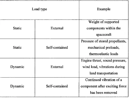
To provide a satisfactory mechanical design for the refrigeration system, we require knowledge o f the mechanical environment to which the spacecraft will be subjected. Structural loads upon the spacecraft will be o f several forms and are summarized in Table 1-1 below"^.

Load type Example

Static External

Weight o f supported components within the

spacecraft

Static Self-contained

Pressure o f stored propellants, mechanical preloads,

thermoelastic loads

Dynamic External

Engine thrust, sound pressure, wind load, vibrations during

land transportation

Dynamic Self-contained

Continued vibration o f a component after exciting force

has been removed

(26)

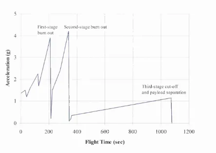
Launch generates the greatest loads for most structures, but any other event can be critical for parts o f the structure. The highest acceleration during a typical Ariane 4 launch is around 4.2g as shown in Figure 1-1 below (load factor of 4.2) Dramatic spikes in acceleration, which represent the launch vehicle’s dynamic response to transients, are observed at certain times such as when the first stage bums out and the second stage ignites. The deterministic loads upon the structure can be predicted as a function o f time by analysing the transmission o f (usually sinusoidal) vibrations from the base o f the spacecraft. Random loads such as due to acoustic pressure can only be estimated statistically.

5

First-stage Secon d -stage bum out bum out

4

3

2

Third-stage cut-off' and payload separation

0

600 800 1000 1200

0 200 400

Flight Time (sec)

Figure 1-1 : Axial acceleration profile for Ariane 4

(27)

Chapter 1 Introduction to Space Cryogenics_________________________________ 25

vibrations. In this analysis, we attempt to find both the most suitable materials and the best geometric configuration o f the system. For a refrigeration system, the best material is determined not ju st by mechanical properties such as density. Y oung’s Modulus, and tensile and compressive yield stresses but also by thermal properties such as thermal conductivity.

The large range o f temperatures the materials must operate under further increases the complexity o f the design, as both mechanical and thermal properties vary with temperature. The system outlined in this thesis will cool from around 300 K to 0.01 K (a factor o f 30000 decrease in absolute temperature).

The thermal conditions under which the refrigeration system must operate are discussed in Section 1.2.2 below.

1.2.2 The thermal environment

It is a common misconception that it is always cold in space. In fact, the temperature varies greatly between around 2.73 K in deep space when isolated from all radiation, and around 300 K for a body orbiting the Earth in direct view o f the sun. O f course, higher temperatures still are obtained by bodies closer to the sun. Recall from Section

1.2 above that the daytime surface temperature o f Mercury is 350 °C - i.e. 623 K. The temperature at the surface o f the sun is 5800 K.

(28)

Component Minimum

Temperature (°C)

Maximum Temperature (°C)

Electronic equipment (operating) -10 +40

Batteries -5 +15

Fuel (e.g. hydrazine) +9 +40

Microprocessors -5 +40

Bearing mechanisms -45 +65

Solar cells -60 +55

Solid-state diodes -60 +95

Table 1-2: Temperature tolerances o f typical spacecraft components

The components o f thermal radiation incident upon the spacecraft are discussed in Section 1.2.2.1 and illustrated in Figure 1-2 below. The emission o f heat fi’om the spacecraft to space is discussed in Section 1.2.2.2. Heat is also transferred between warm and colder parts o f the spacecraft.

1.2.2.1 Components of thermal radiation Incident upon spacecraft

(29)

1.2.2.1.1 Solar radiation

This is radiation emitted by the sun that is directly incident upon the spacecraft. The spectral energy distribution of the sun resembles a Planck curve^ with effective temperature 5800 K, which means that 99% o f the solar energy has wavelengths between 150 nm and 10 /jm with a maximum at around 450 nm.

Radiation from Spacecraft

Solar Radiation

t

Albedo Radiation Planetary

Emissions

Figure 1-2: Components o f radiation incident upon spacecraft

With the total power output o f the sun, P = 3.8 • 10^^ W , the solar radiation intensity,

(30)

The solar radiation falling at right angles onto an area o f 1 at a distance o f 1 AU («150 million km) from the sun, Js,p, is approximately 1371 W/m^ and is called the solar constant. The total power input, , to the satellite from solar radiation is then given by the sum o f the power absorbed by each o f the spacecraft’s surfaces:

where Ai^s is the projected area o f the surface / in the direction o f the sun and or, is the absorptance o f the spacecraft surface material to short wavelength solar radiation.

1.2.2.1.2 Planetary radiation

This is the thermal radiation emitted by the planets due to their temperatures. The planets behave as black body radiators and the Earth emits predominantly infrared radiation with a wavelength greater than 1.5 /mi.

At satellite altitudes, it is reasonable to assume that the planetary radiation emanates from the entire surface o f the planet. Although planetary emissions vary seasonally and with latitude, long-term averages provide an adequate approximation for thermal design o f spacecraft, with a figure o f Jp = 231 W/m^ generally used for the Earth.

(31)

[ 1 . 3 ] _^2

nx

where ^ and ^ are the angles between a line joining the two surfaces and the normals to the respective surfaces. The power input to surface i o f the spacecraft due to planetary emissions is then:

[ 1 4 ] =

where Fp^i is the view factor between the planet and the surface, Ai is the area o f the surface and at,p is the absorptance o f the surface material for planetary (long- wavelength) emissions. In fact, for long-wavelength radiation, the surface absorptance is approximately equal to the surface emissivity, £■,. The total planetary radiation absorbed by the spacecraft is therefore:

[ 1 - 5 ] Q ^ = Y , J p - F , y A , - s ,

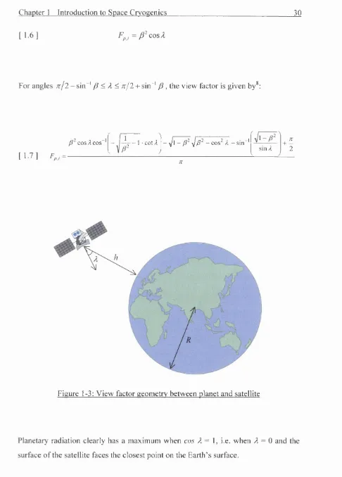
To find the view factor between a spherical planet and a spacecraft surface, the surface is modelled as a flat plate. The view factor then depends on the angle, A, between the normal to the plate and the local vertical on the planet surface, the altitude o f the spacecraft, h, and the radius o f the Earth, R (see Figure 1-3 below).

Writing P = —^ — , the view factor for angles 0 < A < ;r/2 - sin"^ p is given by*:

(32)

[ 1.6 ]

For angles f c j l - s \ n ' yS < ^ < ;r/2 + sin ' , the view factor is given by*

P~ COS A cos"

[ 17 ] Fp, =

- I-V -1 cot A - l / ' - -\p^ -c o s^ /l - sin '

sin/I V

n

+ —

2

Figure 1-3: View factor geometry between planet and satellite

(33)

1.2.2.1.3 Albedo radiation

Some solar radiation reflects o ff the Earth before reaching the spacecraft. Planetary albedo, a, is the fraction o f the incident solar radiation reflected from the planet.

[ 1.8 ] J „ = a- J_{s , p}

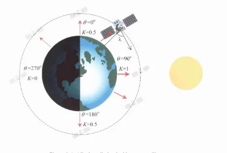
Earth’s albedo varies with surface conditions - for clouds it is 0.8 whereas for forests and fields it ranges from 0.03 to 0.3.^ The average albedos o f the planets o f the solar system and the moon are compared in Table 1-3 below. As for planetary radiation described above, the amount o f albedo radiation that is incident upon a spacecraft is a function o f its altitude and attitude. The geometric view factors for planetary radiation also apply for albedo radiation. They must be adapted, however, to account for the brightness o f the part o f the Earth’s surface visible to the satellite. This is shown in Figure 1-4 below.

Mercury 0.06

Venus 0.61

Earth 0.34

Mars 0.15

Jupiter 0.41

Saturn 0.42

Uranus 0.45

Neptune 0.52

Pluto 0.16

Moon 0.07

(34)

^=0.5

I 6! =90" \

<9=270

K=OJ

Figure 1-4: Albedo radiation incident on satellite

The visibility factor for albedo radiation is defined as the proportion o f albedo

radiation intercepted by the spacecraft. The visibility factor, F, can be defined as some fraction, K, o f the view factor, Fpj.

[ 1 . 9 ] F = K F ._p,i

where 0 < AT < 1. The value o f K can be made to take the values required by writing:

(35)

The total albedo radiation incident upon the surface z, Ja,i, is therefore:

[ 1 1 1 ] =

and the total albedo radiation absorbed by the surface is:

[ 1 1 2 ] Q , a = J . y A - a , ,

where at,a is the absorptance o f the spacecraft surface material for albedo radiation. Since albedo radiation is simply reflected solar radiation, the absorptance o f albedo radiation will be the same as the absorptance o f solar radiation, a,.

We can therefore write an expression for the total albedo radiation absorbed by the spacecraft:

[ 1 1 3 ]

(36)

Chapter 1 Introduction to Space Cryogenics__________________________________M

1.2.2.2 Radiation of heat to

co/d

space

As shown in Figure 1-2 above, the spacecraft also radiates heat to cold space. This has a residual temperature o f 2.73 K from the big bang. Cold space can therefore be modelled as a 2.73 K black body for precise calculations, although it is considered to be a 0 K black body for most approximations.

Heat loss occurs over the entire surface o f the spacecraft, although passive radiators are designed for the specific purpose o f reducing surface temperature. I f surface / o f the spacecraft is at temperature 7}, the heat radiated by the spacecraft to cold space (at temperature To) is given by Stefan’s Law^ as:

where Ai is the area o f the surface /, £/ is the emissivity o f the surface material and cr is the Stefan-Boltzmann constant with value 5.67 10“* W m'^K'"^.

We assume for now that there is negligible heat generated internally within the spacecraft and that the spacecraft uses no active or cryogenic cooling systems (which are described in Sections 1.4.2 and 1.4.3 below respectively). The spacecraft’s equilibrium surface temperature will then be that temperature at which the heat radiated from the spacecraft, , is exactly balanced by the heat incident upon the

spacecraft due to solar, planetary and albedo radiation, Q.„ = f t + 2 ^ + ôa •

(37)

Chapter 1 Introduction to Space Cryogenics_________________________________ ^

the subject o f Section 1.3. This is followed in Section 1.4 with a description o f the technologies available for achieving these temperatures.

1.3 The need for cryogenic temperatures in space

At present, the main requirement for space cryogenics is to improve the precision o f sensing equipment. Generally, “the requirement for cryogenic cooling in space revolves around the need to reduce ‘noise’ and fundamental principles o f detector physics”^. The need for cryogenic temperatures in space is well-documented^’^® and will not be covered in detail here. Examples o f technologies that require cryogenic temperatures are any detectors employing superconductivity (such as superconducting tunnel junctions - STJs), which will not operate at all above their critical temperatures, and bolometric x-ray detectors, which detect quanta o f heat and have an energy resolution that is proportional to The lower we can keep the temperatures o f these detectors, the lower the energy o f the radiation that can be detected (and therefore the more distant the sources that can be resolved). Cryogenic temperatures are also required by infrared sensors on satellites, with applications such as military surveillance and environmental monitoring (including the ozone hole and greenhouse gases/pollution).

(38)

Nevertheless, there have been countless successful sounding rocket and orbital

spacecraft missions employing a variety o f cooling technologies (see Section 1.4 and

Figure 1-6). In 1983, the Infrared Astronomical Satellite, IRAS, carried liquid helium

(see Section 1.4.3.1.1) into orbit for the first time, spending 300 days in space and

maintaining a temperature below 1.8 K. Further successes with liquid helium include

the Cosmic Background Explorer mission (COBE) in 1989, which achieved 1.5 K for

306 days, and the Superfluid Helium On Orbit Transfer mission (SHOOT). This

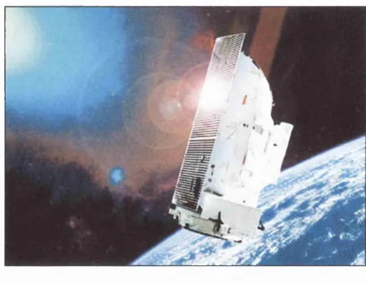
proved the feasibility o f topping up liquid helium supplies during orbit. The

extremely successful Infrared Space Observatory (ISO) was launched in 1995 and is

shown in Figure 1-5 below. ISO operated successfully for 863 days. Mechanical

coolers (see Section 1.4.3.2 below) have also been successfully used in space since

the Improved Stratospheric And Mesospheric Sounder (ISAMS) mission in 1991.

A

Figure 1-5: ISO spacecraft1 2

Despite the successes o f previous missions, none has achieved a temperature

approaching those that will be required by the next generation o f space detectors. The

(39)

1.3.1 The need for 10 mK refrigerators in space

As detector technology becomes more and more advanced, it demands lower and lower temperatures, requiring increasingly sophisticated cooling systems to minimize noise and to maximize energy resolution. There is therefore a constant drive to develop refrigeration systems capable o f cooling to millikelvin temperatures^^. A summary o f the lowest temperatures achieved or required in space for past and future missions is given by Figure 1-6 below^.

Several new detector technologies require cooling to 100 mK and below. These include superconducting tunnel junctions (STJs) and superconducting transition edge sensors (TESs)^^. Current and future space missions already demand sub 100 mK temperatures, with the most recent (unsuccessful) launch, ASTRO-E, requiring 65 mK. Within the next ten to twenty years, the NASA observatory, Constellation-X^^, and the European Space A gency’s (ESA’s) X-ray Evolving Universe Spectroscopy mission (XEUS*"^) will demand 50 mK and 30 mK respectively.

100

Visible/IR Radiometer Various

g -a

i

_g 1

2

IRAS COBE

1975 1980 1985 1990 X 1995 2000 2005 2010 IRTS

Year

ASTRO-E

XEUS

0.01

(40)

Chapter 1 Introduction to Space Cryogenics__________________________________^

Since the requirements o f XEUS most closely match the capabilities o f the refrigeration system developed here at Mullard Space Science Laboratory (MSSL), it will be described in Section 1.3.1.1 below in some detail.

1.3.1.1 XEUS

The XEUS mission planned for launch in 2010-2015 will require cooling to 30 mK and will probably employ either STJs or TESs. The refrigeration system presented here aims to exceed the requirements o f XEUS. The specifications for XEUS are therefore used as a benchmark throughout the design study.

The XEUS mission aims to place a permanent x-ray observatory in low Earth orbit (LEO) with a telescope aperture equivalent to the largest ground-based optical telescope built to date’^. The payload o f XEUS will include three x-ray imaging spectrometers. Firstly, there will be a wide field imager (WFI), using charge-coupled devices (CCDs) at around 150 K. In addition to this, there will be two cryogenic imaging spectrometers (CISs) with operating temperatures between 30 mK and 200 mK. The x-ray observatory will be operated continuously for periods o f around 5 years between successive rendezvous with the International Space Station (ISS).

The XEUS project identified four target science areas*®:

i. The behaviour o f matter under strong gravity, near the event horizons o f black holes

ii. The exploration o f distant objects and the evolution o f the high-energy universe

iii. The creation and redistribution o f the elements

(41)

Chapter 1 Introduction to Space Cryogenics_________________________________ ^

The temperature o f 30 mK is required by the CISs to give an extremely high energy resolution. This represents a considerable challenge, and will require a refrigeration system superior to any that has been flown to date. Existing technologies for cooling in space are described in Section 1.4 below.

1.4 Cooling technologies for space

Thermal control for the spacecraft as a whole is usually achieved by a combination o f active and passive cooling systems. Passive systems, such as radiators, require no power and no feedback control, and operate continuously. Active systems such as thermostatic heaters, on the other hand, may use power-consuming mechanical or thermoelectric devices and often have moving parts. They are therefore inherently less reliable than passive systems.

The systems required for maintenance o f a stable spacecraft temperature are inadequate for providing cryogenic cooling for components that require particularly low temperatures. Even if a radiator were shielded from all radiation and insulated from conducted heat indefinitely (which could never happen in practice), it could only ever achieve a temperature approaching that o f deep space at To, i.e. 2.73 K. This is because the cooling power, , in Equation [ 1.14] becomes zero when T = Tq. In

fact, the lowest temperature that can be achieved with typical radiators^ is around 60 K. In order to achieve the detector temperature o f 10 mK required, therefore, specialized cryogenic refrigeration techniques are needed.

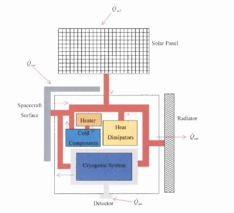
Figure 1-7 below is a schematic showing the heat flows in a basic spacecraft and the relationship between passive, active and cryogenic refrigeration systems. Red arrows represent positive heat flows and blue arrows represent negative heat flows.

Heat flows into the spacecraft from solar radiation absorbed by the surface material

(42)

components such as electronics, and escapes from the spacecraft via the

passive (or active - see Section 1.4.2.1) radiator. Cold components that must be kept

warm to operate (recall Table 1-2) are heated by active thermostatic heaters (see

1.4.2.2). In order to maintain the detectors, which receive power input at the

desired temperature, a cryogenic cooling system is required. This cryogenic system

may either be pre-cooled by the passive radiator or else take heat out o f the system to

assist the radiator, depending on the format o f the cryogenic system and the

prevailing operating conditions. Passive, active and cryogenic refrigeration systems

are described in Sections 1.4.1, 1.4.2 and 1.4.3 respectively.

Qs o l

Spacecraft

Surface

Solar Panel

t

Heater ----

r-H----,_

f1

Heat Dissipators Cold

Components

Cryogenic System

Radiator

a

Detector d el

(43)

Chapter 1 Introduction to Space Cryogenics__________________________________41

1.4.1 Passive refrigeration systems

Passive thermal control systems operate by using materials and surface finishes chosen so that the temperature remains within acceptable limits for the range o f orientations and incident radiation levels expected during the spacecraft’s lifetime^. A simple example o f a passive system is a space radiator thermally coupled to heat generating components by conductive paths.

1.4.1.1 Passive radiators

As described in Section 1.2.2.2 above, heat can be radiated by a hot body to its colder surroundings. This effect is employed by passive radiators. Heat flows from heat dissipating equipment to a specially designed radiator with large surface area.

Traditional radiators have been constructed from honeycombed aluminium panels, although Carbon - Carbon (C-C) composite radiators are currently being developed in the United States*^. C-C is a composite material with pure carbon used for both the reinforcing fibres and the matrix (see Figure 1-8 below). This yields a material with high thermal conductivity in all directions, high strength and a density o f only 65% o f that o f aluminium. Furthermore, unlike mechanically inferior honeycombed aluminium, C-C can be used as a structural material itself, not ju st as a covering for the surface o f the underlying structure. Research so far suggests that C-C, which is currently used on the leading edge o f Space Shuttle wings, may soon feature in a wide range o f spacecraft components, including radiators, battery sleeves and electronics boxes^^.

(44)

The amount o f cooling power that can be provided by a passive radiator at

temperature T is a function o f the difference between the total incident radiation

falling upon the spacecraft and the heat radiated into cold space by the spacecraft.

This cooling power is required to compensate any heat generated internally within the

spacecraft as well as providing any pre-cooling o f cryogenic refrigeration systems.

Figure 1-8: Carbon - Carbon (C-C) radiator16

Equation [ 1.14 ] in Section 1.2.2.2 above gives the amount o f heat emitted by the

spacecraft to cold space. The total radiation incident upon the spacecraft due to solar,

planetary and albedo components is given by:

[ 1.15] _{Qin - Q s ^ Q p ^ Q a}

and from [ 1.2 ],[ 1.5 ] and [ 1.13 ], the radiation incident on the surface is

(45)

so the total heat absorbed by the satellite is:

[ 1 1 6 ] _A,s_{+ 4}

The cooling power, , can then be obtained from Equations [ 1.14 ]

and [ 1. 16] . Approximating the temperature o f deep space, To, to be zero:

[ 1 1 7 ] = E

\

V y

Passive radiators are designed to maximize the heat radiated from the spacecraft and

minimize the heat absorbed. This is achieved by using a large area radiator made

from a material with a low absorptance to emissivity ratio {c d é ) and by linking the

radiator thermally to the heat generating components o f the spacecraft. This way, as

much heat as possible is made to flow to the radiator so that it can be radiated to deep

space. Performance o f passive radiators is obviously greatly affected by the

orientation o f the spacecraft with respect to the planets and the sun, the position o f the

radiator and the orbit o f the spacecraft.

Consider the cooling power o f a passive radiator operating at 150 K, the operating

temperature for the first spectrometer on XEUS^"^. Assuming that the spacecraft

attitude is controlled so that the radiator never faces the sun, the projected area o f the

radiator in the direction o f the sun, Ar,s, is zero. The cooling power o f the radiator,

(46)

[ 1 . 1 8 ]

which can be expressed in words:

Q r =

heat emitted incident planetary incident albedo

by radiator radiation radiation

For a large two-stage radiator'^ o f surface area A r= 12 with emissivity £>• = 0.9 and temperature Tr= 150 K, the heat emitted by the radiator (the first term o f [ 1.18 ] above) becomes 310 W.

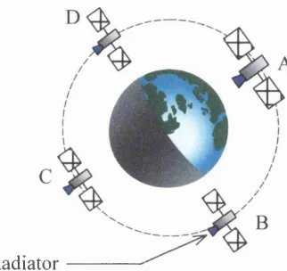
The remainder o f Equation [ 1.18 ], i.e. the incident radiation, will depend on the orientation o f the radiator with respect to the planet and the sun. When the radiator faces away from the planet (as at point C in Figure 1-9 below) so that Fp^ = 0, the cooling power has its maximum value o f 310 W. If the radiator were ever to face the planet directly with the sun behind (as at point A in Figure 1-9 below), then the planetary and albedo power inputs would both be maximum (with cos X = \ and K =

1). The cooling power o f the radiator would therefore have a minimum.

I f we assume that the absorptance o f the radiator ov = 0.2, the Earth’s planetary emissions Jp = 231 W/m^, the LEO altitude h = 700 km, the radius o f the Earth R = 6380 km, the solar radiation J,s,p 1371 W/m , and Earth’s albedo a = 0.34, then

cos>^

Equation [ 1.6 ] gives ^ = 0.81 for maximum heat input.