THE EFFECTIVENESS OF CHINA’S MONETARY POLICY: BASED ON
THE MIXED-FREQUENCY DATA
Deqing Wang1+
Yinqiu Song2
Hongyan Zhang3
Shengjie Pan4
1,2,3,4School of Economics and Management, University of Chinese Academy of Sciences, Beijing, China.
(+ Corresponding author)
ABSTRACT
Article History Received: 29 November 2019 Revised: 16 January 2020 Accepted: 19 February 2020 Published: 24 March 2020
Keyword
s
Monetary policy China Effectiveness New normal Mixed-frequency FAVAR Bayesian. JEL Classification: C32; E52.After the period of rapid growth, the Chinese economy has entered the ―new normal‖ stage. This is a sign of the expected slowdown in economic growth. In the course of development, has the effectiveness of China‘s monetary policy changed? Which of quantity and price rule monetary policies is more suitable for China‘s economy? Very few researches focus on these questions, and this paper constructed a novel Mixed-Frequency Bayesian Factor Augmented Vector AutoRegression (MF-BFAVAR for short) model by combining the dynamic factor model, mixed-frequency spirit, Bayesian estimation, and factor augmented vector autoregression to find the answer. And we applied three different frequencies of data, in order to get the best estimated results. The conclusion is that price rule monetary policy is suitable for the period of steady development, and when economic growth suffers fluctuations, quantity rule monetary policy has better performance. Therefore, monetary policymakers should formulate the most effective policy based on different situations.
Contribution/ Originality:
This study is one of the very few researches on the effectiveness of China‘s monetary policy under the ―new normal‖ situation. And we construct a novel methodology framework, MF-BFAVAR, which is, as far as we know, the first time to take advantage of the dynamic factor model, mixed-frequency spirit, Bayesian estimation and factor augmented vector autoregression at the same time. Unlike the existing literature, we applied data at three different frequencies (quarterly, monthly and daily) in our estimation.1. INTRODUCTION
China, as one of the world‘s most notable economies, has achieved amazing economic development. Since the year of 2014, the growth rate of China‘s GDP has been turned from ―high‖ to ―medium high‖. One obvious sign is that expected growth rate of GDP have been downshifted from around 10% to a 6-7%. The Chinese President Xi Jinping applied the term ―new normal‖ to describe the situation in 2014. Since then, it has been used not only to describe slower economic growth, but also to describe the changes taking place in China‘s economy generally, such as intelligent manufacturing, poverty eradication, stricter environmental regulations (Abdul-Rahaman & Yao, 2019;
Aizenman, Chinn, & Ito, 2016; Chen & Groenewold, 2019; Mi et al., 2017).
The ―new normal‖ of Chinese economy is a hot topic, and related research is growing rapidly. However, there are very few researches on the changes of effectiveness of Chinese monetary policy under the condition of ―new normal‖ (Abdul-Rahaman & Yao, 2019; Aizenman et al., 2016; Kang, 2018; Zhang, Chen, Fan, & Wang, 2018). In
Asian Economic and Financial Review
ISSN(e):
2222-6737 ISSN(p):
2305-2147
DOI: 10.18488/journal.aefr.2020.103.325.339 Vol. 10, No. 3, 325-339.
China ‘s latest 14th five-year development plan, the important role of monetary policy in macroeconomic regulation and control has once again become prominent. Prior to the 2008 financial crisis, China has formed a monetary policy framework that is primarily based on quantity rule and supplemented by price rule. At the same time, China has spared no effort to promote the process of marketization of interest rates (Zhao, Wang, & Deng, 2019). In 2015, the marketization of interest rates was basically completed, which provided favorable conditions for the effective implementation of price rule monetary policy (Ausloos, Ma, Kaur, Syed, & Dhesi, 2019; He, Leung, & Chong, 2013;
Tan, Ji, & Huang, 2016). In fact, since the reform and opening up, China's economic structure has undergone several
tremendous changes. In the course of decades of development, the effectiveness of China's monetary policy has also changed alongside with the rapid economic growth. Since the Chinese economy entered the "new normal" situation, has the effectiveness of different monetary policies changed in response? Which monetary policy rule should be selected as the main implementation one in the future? This paper is trying to give the answer.
However, doing research on China‘s monetary policy is not easy, due to the not very satisfactory quality of statistical data, such as the lack of long-term historical data. And the rapid institutional and structural changes that China has undergone also have an impact on the quality (Fernald, Spiegel, & Swanson, 2014; He et al., 2013; Liu,
Song, & Huang, 2019). Moreover, in previous studies, the common macroeconomic data used in analysis with low
statistical frequency usually. GDP, as an example, is quarterly frequency. Limited by the statistical frequency, many useful indicators of economy cannot be included in the analysis model. Although there are some attempts to use mixed frequency data, the data used for research contains only two kinds of statistical frequencies (e.g. monthly-quarterly or weekly-monthly). Insufficient indicators will not reflect the full picture of economy status. Therefor we design a novel MF-BFAVAR (Mixed Frequency Bayesian Factor Augmented Vector Autoregression) method with three kinds of frequency data (quarterly-monthly-daily) to solve the data problems, in order to get better estimation. Our results show that the price rule monetary policy had a better performance for the whole-time span and the period with steady economic growth. While the quantity rule monetary policy could inject power for the period of volatile economic growth.
The follow-up content of our paper is designed as follows. Section 2 is literature review, which details the research progress in related areas. Section 3 introduces the innovative methodology adopted in this paper. Section 4 shows the data we used and the empirical results we got. At last, Section 5 is conclusion.
2. LITERATURE REVIEW
As mentioned above, the ―new normal‖ of Chinese economy is a hot topic. Through a systematic review of existing literature, Tung (2016) made a detailed analysis of the opportunities and challenges that China's future development facing with the ―new normal‖ situation, from many perspectives including foreign exchange reserves and financial development, regional economic integration and development, large-scale scientific and technological innovation and upgrading. Chen and Groenewold (2019) design a framework that combines the VAR model and Blanchard-Quah identification procedure to identify the primary cause affecting China‘s economic slowdown. And their results show that the slowdown has been mainly supply-driven.
However, there are very few researches on the changes of effectiveness of Chinese monetary policy under the condition of ―new normal‖. Zhang et al. (2018) propose an innovational time-varying parameter vector autoregression, combined with data mining technology, to in investigate the time-varying effectiveness characteristics of China‘s monetary policy, with monthly data. The empirical estimation results of Kang (2018)
impact of the ―new normal‖ on Chinese economy and various sectors. The conclusion of the study shows that the gradually tightening monetary policy will have very little effect on economic development in the long run, but the decrease in savings will have an adverse effect on it in the short term. The liberation reform will promote the appreciations of the RMB to a certain extent.
Turn to the methodology. The typical VAR model is one of the most popular tool in the area of monetary policy. But it has many shortcomings. Limited by the degree of freedom, the typical VAR model can only contain a few variables. But we cannot count on one official statistical indicator to perfectly reveal entire information (such as GDP and output, CPI and inflation). This greatly affects the estimation performance of the model. The FAVAR model constructed by Bernanke, Boivin, and Eliasz (2005) using a structural VAR model combined with the factor analysis model for large scale of data makes up for these shortcomings. The main advantage of the FAVAR model is that it can get rid of the limitation of the number of variables in the traditional VAR model while maintaining the general VAR analysis function. Furthermore, the FAVAR model, which can accommodate much more information, is more similar with the real situation central banks and policymakers face, and can minimize the problem of mismeasurement. In addition, the FAVAR model focuses more on reflecting the trend of a set of indicators, and high quality of data is not required. Due to the quality of Chinese statistics is not very well, the FAVAR model is much suitable for our demands. Moreover, many previous literatures have proven that the FAVAR model performs well in empirical estimation, even for relatively reliable data (Bernanke et al., 2005; He et al., 2013). Therefore, the FAVAR model has been widely used, especially in the macroeconomics area, and extended many novel models.
Mumtaz and Surico (2009) followed the FAVAR method of Bernanke et al. (2005) using a large amount of
panel data from 17 industrialized countries to study the global transmission mechanism of anomalous shocks and its impact on the United Kingdom. Bai and Ng (2013) constructed a novel method for extracting latent factors by innovating the principal component analysis approach under restricted conditions, and then proposed a new FAVAR model. Claeys and Vašíček (2014) constructed a new shock conduction monitoring research framework by combining the structural break test and FAVAR model which Qu and Perron (2007) proposed. It also took the sovereign bonds markets of the 16 EU countries as research objects and investigated the transmission Channels of the financial crisis in these bond markets.
There is also no lack of research on China's monetary policy. For example, Fernald et al. (2014) demonstrated the excellent performance of the FAVAR model for research with China's economic data, and used this method to conduct an empirical estimation of the transmission path of China's monetary policy. The results show that increasing bank reserve requirements will reduce economic activity and inflation. Because China‘s central bank determines changes in interest rates, it has a direct impact on economic activity and inflation. And China's monetary policy transmission mechanism is gradually closer to the Western market economy. In addition to the monetary policy, FAVAR has also been used in many other areas of research, such as identifying coal market shocks
(Chevallier, 2011) exploring factors affecting oil prices (Aastveit, Bjørnland, & Thorsrud, 2015) and the
transmission mechanism of shocks in the cryptocurrency market (Antonakakis, Chatziantoniou, & Gabauer, 2019). The FAVAR model also extends many new branches. Integrated with time-varying parameters, as an instant,
Liu et al. (2019) constructed the TVP-FAVAR model to study the dynamic changes of China's monetary policy over
time. It convinced that China's monetary policy has time-varying characteristic. Price rule and quantity rule have their own advantages, and they should be implemented based on different policy objectives. Since the 2008 global financial crisis, price rule monetary policy has been more suitable for the development of Chinese society.
The Bayesian FAVAR approach combined with the Bayesian Inference and FAVAR, shows a better performance in existing papers. For example, Gunter and Önder (2016) constructed a Bayesian FAVAR model, and used the traffic big data obtained from 10 Google Analytics websites to predict the actual visitors to Vienna. Serati
and Venegoni (2019) constructed a new type of Bayesian Time-Varying Parameters FAVAR to study the changing
debt crisis have changed the transmission channels of the Eurozone monetary policy, both on price rules (interest rates) or quantity rules (credit). The coordination of fiscal and monetary policies needs to be strengthened in order to exert the best policy results.
Another drawback of the classic VAR model is that it can only do research with the same frequency data, but the statistical frequency of economic data is various. Macroeconomic data are almost quarterly and monthly, while the frequency of financial market statistics is higher. This causes the traditional VAR model to fail to cover more statistical indicators, which will make it difficult to effectively reflect the full picture of the information.
Thus, the Mixed-Frequency VAR method rose in response to these conditions. The spirit of mixed-frequency comes from two articles by Mariano and Murasawa (2003); Mariano and Murasawa (2010). Based on articles that
James and Watson (1988); Stock. and Watson (1989); Stock and Watson (1998); Stock and Watson (2002) using
dynamic factor models to construct consistent factor, Mariano and Murasawa added maximum likelihood estimation to build mixed frequency dynamic factor model that included both monthly and quarterly data. This has also become the origin of various mixed-frequency models, laying a foundation for subsequent related research. Based on these articles, the mixed-frequency model has also been developed in the fields of prediction, shocks identification and transmission. However, whether MF-VAR or MIDAS, the different branching methods, is better have been debated in academia. Schorfheide and Song (2015) integrated the Bayesian method to MF-VAR to construct the Bayesian MF-VAR model with quarterly and monthly data, and compared it with the traditional VAR model and MIDAS regression method. They proved empirically that the new method performed better. Baumeister,
Guérin, and Kilian (2015) used the MIDAS regression model and mixed data to explore the linkages between the
financial markets and the oil markets. And their results show that the weekly financial market data had a leading significance for the monthly oil price. According to the finding their prediction of the monthly oil price, compared to the VAR model, is considerable better. In sum, it is generally convinced that the effectiveness of the MF-VAR model is limited by the curse of dimensionality, so it is sometimes slightly inferior to that of MIDAS model. However, with the same constraints, the MF-VAR model performs better (Kuzin, Marcellino, & Schumacher, 2011). Therefore, if the above FAVAR model is introduced, the problem can be solved easily.
Nevertheless, so far, we found that although FAVAR and mixed-frequency factor models both inherit the spirit
of James and Watson (1988); Stock. and Watson (1989); Stock and Watson (1998); Stock and Watson (2002) the
studies using mixed-frequency data combined with FAVAR models is scarce. There are only two articles in the SCI-E and SSCI core database. Moench and Ng (2011) extracted the common component from the mixed-frequency data, and combined with the FAVAR model to explore the connection between US housing and consumption.
Marcellino and Sivec (2016) extended the MF-VAR model to the MF-FAVAR model and incorporated Monte
Carlo estimation method to reproduce existing researches (Bernanke et al., 2005; Bernanke., Gertler, Watson, Sims,
& Friedman, 1997). These results show that the innovative method improves the ability to identify shocks, avoids
biased estimation caused by missing information, and has better calculation results.
In the process of estimating, they both used quarterly and monthly data, just like the previous studies. However, in recent years, a large amount of data is produced in various departments every day, and high-frequency data and big data show a blowout state. The existing method not including higher frequency data will miss many useful information.
3. METHODOLOGY
In this section, we construct a methodology framework for our empirical estimation. And we gave the novel framework a name MF-BFAVAR (Mixed-Frequency Bayesian Factor Augmented Vector AutoRegression). It integrates mixed-frequency spirit, dynamic factor model, Bayesian method and VAR model.
3.1. Dynamic Factor Model
The dynamic factor model is the method for extracting underlying factors, and we use the presentation way of
Fernald et al. (2014) and Liu et al. (2019) in this paper. Let F is a small number of potential factors that we cannot
observe from economic activities. X is an N-dimensional multivariate time series vector, which determined by F.
And X is composed of data that we can specifically observe in actual economic activities. And is the 0 mean
idiosyncratic errors, which is mutually orthogonal stationary process with F. For T periods, the original dynamic factor model can be defined as follows:
. (1)
In the Equation 1, scale of the vector is much larger than that of the vector . And is the loadings matrix
of the indicators X on the factors F. In the dynamic factor model, the factors F are related over time, typically according to a linear autoregression process (as shown in Equation 2):
, (2)
Where A(L) is the polynomial containing lag operators.
3.2. The Spirit of Mixed-Frequency
As mentioned in the section 2, for the general VAR or FAVAR model, it is not difficult to deal with the same frequency and time span data.
However, due to the different frequencies and time span of macroeconomic statistics, not to mention the quality of Chinese data, it is hard to count on a single statistic indicator to reflect the overall economic status. In addition, because of the different frequencies data cannot be taken, there are some important indicator cannot be considered, which will inevitably lead to the omission of information. Therefore, this paper refers to the method applied by
Mariano and Murasawa (2003); Mariano and Murasawa (2010) to introduce the spirit of mixed-frequency into our
methodological framework.
Let be the high-frequency latent factor of the observable variable . In this case, is quarterly data,
and are its monthly latent factors. Then the variable can be observed once every three months, which can
be expressed as the geometric mean of its three latent factors. As shown in Equation 3:
. (3)
And for all t, let . Then we can get Equation 4:
So is an indicator that can be observed every three months, and is an unobservable indicator.
For all t, let , and . We can get Equation 5 and Equation 6:
, (5)
, (6)
where L is the lag operator. The Equation 5 can be transformed into a Gaussian or General VAR model with p order (as shown in Equation 7),
, . (7)
For , we define the state vector as . The state space representation can be expressed
as Equation 8 and Equation 9,
, , (8)
, (9)
where , , . And is the
mixed-frequency series we calculated. Nevertheless, on account of the missing values of our results, factor extraction cannot be implemented directly. To solve the problem, we referred to the approach in existing studies
(Harvey, 1990; Kuzin et al., 2011; Mariano & Murasawa, 2003, 2010) introducing the Kalman filter and smoother to
fill the missing values.
Meanwhile, the daily high-frequency data also played a role in our article. However, if the quarterly and monthly data is converted into daily according to the method above, there will be several problems: (i) It is easy to make too much missing data and lead to inaccurate estimations. (ii) The calculation burden is too heavy. Hence, we made an improvement to avoid these problems. That is, monthly is selected as the intermediate frequency, the above formulas are inverted to estimate the latent monthly indicator of the daily data.
3.3. Bayesian Parameters Estimation
Our work referred to the practices of Giannone, Lenza, and Primiceri (2015) and Gunter and Önder (2016)
Minnesota prior is an informative prior that was proposed by Doan, Litterman, and Sims (1984) and Litterman
(1986) and gradually became one of the most popular informative priors (Giannone et al., 2015).
Compared with the parameter estimation method applied by the general VAR model, the assumption of Minnesota prior is that the parameters for any VAR equation are random variables that have the characteristic of random walk with drift process. It turns the restrictions on degrees of freedom to that on more distant variable lags
(Bańbura, Giannone, & Reichlin, 2010). The use of the informative prior shrinks the unconstrained VAR(p) to a
naiver form to obtain a better parameters estimation, which is conducive to better identification and prediction results. In contrast, using uninformative or diffuse priors, such as flat prior, cannot reflect the advantages of Bayesian methods (Giannone et al., 2015).
This paper follows the expression of Lütkepohl (2005) and Gunter and Önder (2016). In Bayesian estimation, it
is first assumed a prior probability density function (PDF) , and the is a common parameter vector without
sample information. Correspondingly, the sample PDF of the with sample information can be given by ,
which is similar to the likelihood function . Let denote the unconditional sample density, and then we
can connect the prior PDF and the sample PDF by the equation:
. (12)
Equation 12 is the so-called posterior PDF, which denotes the distribution of under the sample information
of y. We also can use the likelihood function and prior PDF to represent it:
(13)
The PDF of posterior shown in Equation 13 cannot be computed directly. We should deal with the parameter
vector first to obtain the numerical solution. The parameters to be estimated of vector include the parameters
of the model and three hyperparameters of BVAR(p). In this paper, we set the overall tightness as 0.1, relative cross-variable weight as 0.99, and 1 for lag decay.
3.4. MF-BFAVAR
Finally, we can establish our FAVAR framework (see Equation 14 and Equation 15) in this paper after the works above, as the instrument to identify the effectiveness of monetary policy shocks:
(14)
, (15)
Where is the observable monetary policy variable, is the observable variable, and denotes the latent
factor extracted base on the dynamic factor model with mixed-frequency spirit. A(L) and B(L) denote lag
polynomial with p order and the L is lag operator. and are stochastic disturbances subject to iid. In the process
2010) by implementing the principal component analysis to obtain the latent factors. At the same time, this article
divided the indicators into two groups, to construct the consistency factors of ―output‖ and ―inflation‖, as
Fernald et al. (2014) and Liu et al. (2019) did.
However, information on monetary policy is not perfectly reflected by an observable indicator. Therefore, our
paper makes an improvement on the basis of the typical dynamic factor model, and added the potential variable .
Hence, the FAVAR equation can be modified to Equation 16:
(16)
Where is the latent factor of monetary policy (―quantity rule‖ or ―price rule‖), is is lag polynomial with
p order, and obeys iid. At last, we finished the establishment of the methodology framework, which is the
so-called MF-BFAVAR, as the main tool to identify the shocks of the monetary policy. And we used the same model with different lag period to verify the robustness of our methodology.
4. EMPIRICAL RESULTS
4.1. Data Description
We applied the study framework constructed above (MF-BFAVAR), to measure the changes of effectiveness and transmission mechanism of China‘s monetary policy in different periods. The data we used is with three frequencies: quarterly, monthly and daily. The time span is from January 2000 to December 2019, covering the periods of the rapid development of China before the global financial crisis, the sharp decline during the crisis, the subsequent rapid recovery, and the ―new normal‖ of economy.
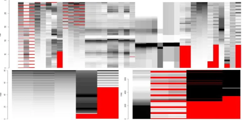
Figure 1 shows the missing values of the indicators we applied. In order to obtain the precise result, it is necessarily to eliminate the effects caused by multiple reasons such as the Chinese Spring Festival. And this article filled in missing values in two ways. For some ―output‖ data, relatively accurate inferences can be made through some relevant indicators.
The missing values of other indicators are filled by the structural time series model and Kalman filter. A R package developed by Moritz and Bartz-Beielstein (2017) was implemented here. And for irregular indicators, such as the deposit reserve ratio, we transferred them to monthly data.
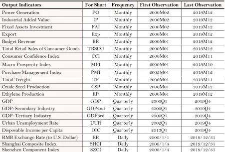
In order to eliminate the effects of price and seasonal changes, this article converts the raw quantitative data into year-on-year growth rates. And all the data is processed by Z-core standardization. The data of the selected 40 indicators details see Table 1-Table 4 are from the China Statistical Yearbook, the database of National Bureau of Statistics of China, and the Choice Economic Database.
Table-1. Description of output indicators.
Output Indicators For Short Frequency First Observation Last Observation
Power Generation PG Monthly 2000M02 2019M12
Industrial Added Value IP Monthly 2000M02 2019M12
Fixed Assets Investment FAI Monthly 2000M02 2019M12
Export Exp Monthly 2000M01 2019M12
Budget Revenue BR Monthly 2000M01 2019M12
Total Retail Sales of Consumer Goods TRSCG Monthly 2000M01 2019M12
Consumer Confidence Index CCI Monthly 2000M01 2019M11
Macro Prosperity Index MPI Monthly 2000M01 2019M10
Purchase Management Index PMI Monthly 2005M01 2019M12
Total Treight TF Monthly 2000M01 2019M11
Crude Steel Production CSP Monthly 2000M01 2019M12
Ethylene Production EP Monthly 2000M01 2019M12
GDP GDP Quarterly 2000Q1 2019Q4
GDP: Secondary Industry GDP2nd Quarterly 2000Q1 2019Q4
GDP: Tertiary Industry GDP3rd Quarterly 2000Q1 2019Q4
Urban Unemployment Rate UUR Quarterly 2002Q1 2019Q4
Disposable Income per Capita DIC Quarterly 2013Q1 2019Q4
RMB Exchange Rate (to U.S. Dollar) ER Daily 2000/1/1 2019/12/31
Shanghai Composite Index SHCI Daily 2000/1/4 2019/12/31
Shenzhen Component Index SZCI Daily 2000/1/4 2019/12/31
Table-2. Description of inflation indicators.
Inflation Indicators For Short Frequency First Observation Last Observation
Consumer Price Index CPI Monthly 2000M01 2019M12
Consumer Price Index: Urban CPIU Monthly 2000M01 2019M12
Consumer Price Index: Rural CPIR Monthly 2000M01 2019M12
Consumer Price Index: Food CPIF Monthly 2000M01 2019M12
Consumer Price Index: Non-Food CPINF Monthly 2002M03 2019M12
Producer Price Index PPI Monthly 2000M01 2019M12
Purchasing Price Index of Raw
Material, Fuel and Power PPIRM Monthly 2000M01 2019M12
Retail Price Index RPI Monthly 2000M01 2019M12
Corporate Goods Price Index CGPI Monthly 2000M01 2019M12
Consumer Price Index: in 36
Table-3. Description of quantity rule indicators.
Quantity Rule For Short Frequency First Observation Last Observation
M0 M0 Monthly 2000M01 2019M12
M1 M1 Monthly 2000M01 2019M12
M2 M2 Monthly 2000M01 2019M12
Table-4. Description of price rule indicators.
Price Rule For Short Frequency First Observation Last Observation
Medium and Long-Term Loan
Interest Rate: 3 To 5 Years (Inclusive) MLLIR Irregular 2000M01 2015M10 Time Deposit Interest Rate: 1 Year
(Full Deposit and Withdrawal)
(Month) RDIR Irregular 2000M01 2015M10
SHIBOR: Overnight SHIBOR1d Daily 2006/10/8 2019/12/31
SHIBOR: 7Day SHIBOR7d Daily 2006/10/8 2019/12/31
Chinabond Treasury Maturity Yield: 1
Year TMY1y Daily 2002/1/4 2019/12/31
Chinabond Treasury Maturity Yield: 5
Years TMY5y Daily 2002/1/4 2019/12/31
CHIBOR: 7 Days CHIBOR7d Daily 2004/5/24 2019/12/31
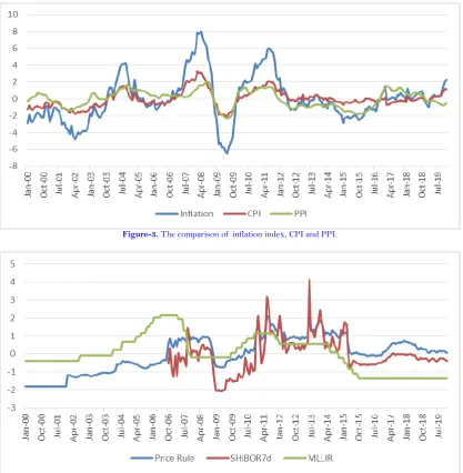
4.2. The Indexes
We used the Kalman filter to integrate the data with mixed frequencies earlier. In this section we use principal component analysis (PCA), another familiar tool of dynamic factor models, to construct the index of each division.
Figure-3. The comparison of inflation index, CPI and PPI.
Figure-4. The comparison of price rule index, SHIBOR7d and MLLIR.
Figure-5. The comparison of quantity rule index, M1 and M2.
4.3. The Results and Discussion
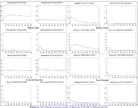
Figure 6 exhibits the impulse response images from the Bayesian FAVAR model by EViews 10.0. They reflect the effectiveness of two rules of monetary policy in different period.
Figure-6. The impulse response results of Bayesian FAVAR in different period.
4.3.1. The Whole Time: 2000-2019
Over the whole-time span, the price rule of monetary policy had a better performance. The response of economic output to a shock of price rule increases from 0 to 0.024, while that of quantity rule increases to about 0.007. And the response of inflation to a shock of price rule increase to 0.078, which is less than 0.161 of quantity rule. For all time, the price rule could accelerate the economic output with less inflation growth.
4.3.2. The Period before the Financial Crisis: 2000-2006
At the beginning of the 20th century, and before the financial crisis, China‘s economy developed steadily and rapidly for severe years. With the continuous progress of market-oriented reforms, the role of price rule monetary policy had become increasingly prominent. As shown in Figure 6, a shock of price rule tools will trigger an increase in economic output of 0.060, which is better than 0.024 of quantity rule. Meanwhile, the contribution of price rule tools (0.230) to inflation is also higher than the quantity rule (0.133).
4.3.3. The Financial Crisis and Recovering: 2007-2014
4.3.4. The Period of “New Normal”: 2015-2019
In the period when the China‘s economy has just entered the ―new normal‖, both monetary policies had a positive effect on economic output. Quantity rule tools are more like a double-edged sword, which is slightly better than price rule in promoting output with more increase of inflation. The price rule is more moderate. From the
Figure 6, giving a shock to quantity rule will cause an increase on economic output to 0.094, which is higher than
0.051 of price rule. And the inflation also makes a growth of 0.015 that is a little bit higher than 0.012 of price rule. We can conclude that, the price rule monetary policy was more effective for the entire time span. It means that China‘s interest rate marketization process had achieved good results, providing a guarantee for the implementation of price rule monetary policy. This summary also coincides with the conclusion of Fernald et al. (2014) that China‘s monetary policy environment is becoming more and more like that of Western economies. Prior to the financial crisis, the advantages of price rule instruments have been highlighted. And during the financial crisis and subsequent recovery phases, more straightforward quantity rule tools are more capable of driving economic recovery. After the Chinese economy entered the ―new normal‖ stage, although the economic growth has declined, the overall development has been relatively stable. Both quantity and price rule policies have demonstrated their own characteristics.
5. CONCLUSION
China‘s interest rate liberalization process ensures the effective implementation of price rule monetary policy. Under this premise, in the period of stable and rapid economic development, the effectiveness of price rule tools is better than that of quantity rule. In less favorable situations, such as decline or fluctuation in economic growth, straightforward quantity rule instruments are more likely to reverse the momentum. Different monetary policies have different dynamic effectiveness corresponding to different situations. As a good example, the U.S. Federal Reserve increased its use of quantity rule instruments after the financial crisis. Therefore, facing with volatile economic situation in the future, the monetary policy is not a binary choice. The policy makers should formulate the most effective policies according to different environments. In future, scholars should consider the impact of global economic changes and the simulations of monetary policy in different situations.
Funding: This study receives the financial support from the general research project (no. Y52902GEB1) of University of Chinese Academy of Sciences.
Competing Interests: The authors declare that they have no competing interests.
Acknowledgement: All authors contributed equally to the conception and design of the study.
REFERENCES
Aastveit, K. A., Bjørnland, H. C., & Thorsrud, L. A. (2015). What drives oil prices? Emerging versus developed economies. Journal of Applied Econometrics, 30(7), 1013-1028. Available at: https://doi.org/10.1002/jae.2406.
Abdul-Rahaman, A. R., & Yao, H. (2019). China's new normal and the implications to domestic and global business. International
Journal of Finance & Economics, 1-15. Available at: https://doi.org/10.1002/ijfe.1737.
Aizenman, J., Chinn, M. D., & Ito, H. (2016). Monetary policy spillovers and the trilemma in the new normal: Periphery country
sensitivity to core country conditions. Journal of International Money and Finance, 68, 298-330. Available at:
https://doi.org/10.1016/j.jimonfin.2016.02.008.
Antonakakis, N., Chatziantoniou, I., & Gabauer, D. (2019). Cryptocurrency market contagion: Market uncertainty, market
complexity, and dynamic portfolios. Journal of International Financial Markets, Institutions and Money, 61, 37-51.
Available at: https://doi.org/10.1016/j.intfin.2019.02.003.
Ausloos, M., Ma, Q., Kaur, P., Syed, B., & Dhesi, G. (2019). Duration gap analysis revisited method in order to improve risk
management: The case of Chinese commercial bank interest rate risks after interest rate liberalization. Soft Computing,
Bai, J., & Ng, S. (2013). Principal components estimation and identification of static factors. Journal of Econometrics, 176(1), 18-29. Available at: https://doi.org/10.1016/j.jeconom.2013.03.007.
Bańbura, M., Giannone, D., & Reichlin, L. (2010). Large Bayesian vector auto regressions. Journal of Applied Econometrics, 25(1),
71-92. Available at: https://doi.org/10.1002/jae.1137.
Baumeister, C., Guérin, P., & Kilian, L. (2015). Do high-frequency financial data help forecast oil prices? The MIDAS touch at
work. International Journal of Forecasting, 31(2), 238-252. Available at: https://doi.org/10.1016/j.ijforecast.2014.06.005.
Bernanke, B. S., Boivin, J., & Eliasz, P. (2005). Measuring the effects of monetary policy: A factor-augmented vector
autoregressive (FAVAR) approach. The Quarterly Journal of Economics, 120(1), 387-422. Available at:
https://doi.org/10.1162/0033553053327452.
Bernanke., B. S., Gertler, M., Watson, M., Sims, C. A., & Friedman, B. M. (1997). Systematic monetary policy and the effects of
oil price shocks. Brookings Papers on Economic Activity, 1997(1), 91-157. Available at:
https://doi.org/10.1016/j.jeconom.2016.04.010.
Chen, A., & Groenewold, N. (2019). China's ‗New Normal‘: Is the growth slowdown demand-or supply-driven? China Economic
Review, 58, 1-22. Available at: https://doi.org/10.1016/j.chieco.2018.07.009.
Chevallier, J. (2011). Macroeconomics, finance, commodities: Interactions with carbon markets in a data-rich model. Economic
Modelling, 28(1-2), 557-567. Available at: https://doi.org/10.1016/j.econmod.2010.06.016.
Claeys, P., & Vašíček, B. (2014). Measuring bilateral spillover and testing contagion on sovereign bond markets in Europe. Journal of Banking & Finance, 46, 151-165. Available at: https://doi.org/10.1016/j.jbankfin.2014.05.011.
Doan, T., Litterman, R., & Sims, C. (1984). Forecasting and conditional projection using realistic prior distributions. Econometric
Reviews, 3(1), 1-100. Available at: https://doi.org/10.1080/07474938408800053.
Fernald, J. G., Spiegel, M. M., & Swanson, E. T. (2014). Monetary policy effectiveness in China: Evidence from a FAVAR model. Journal of International Money and Finance, 49, 83-103. Available at: https://doi.org/10.1016/j.jimonfin.2014.05.007.
Giannone, D., Lenza, M., & Primiceri, G. E. (2015). Prior selection for vector autoregressions. Review of Economics and Statistics,
97(2), 436-451. Available at: https://doi.org/10.1162/rest_a_00483.
Gunter, U., & Önder, I. (2016). Forecasting city arrivals with Google analytics. Annals of Tourism Research, 61, 199-212. Available
at: https://doi.org/10.1016/j.annals.2016.10.007.
Harvey, A. C. (1990). Forecasting, structural time series models and the Kalman filter (pp. 101-112). Cambridge, UK: Cambridge University Press.
He, Q., Leung, P.-H., & Chong, T. T.-L. (2013). Factor-augmented VAR analysis of the monetary policy in China. China Economic
Review, 25, 88-104. Available at: https://doi.org/10.1016/j.chieco.2013.03.001.
James, S. H., & Watson, M. W. (1988). A probability model of the coincident economic indicators. Mass., USA: National Bureau of Economic Research Cambridge.
Kang, C. (2018). China's monetary policy under the" new normal". China: An International Journal, 16(3), 74-96.
Kuzin, V., Marcellino, M., & Schumacher, C. (2011). MIDAS vs. mixed-frequency VAR: Nowcasting GDP in the euro area. International Journal of Forecasting, 27(2), 529-542. Available at: https://doi.org/10.1016/j.ijforecast.2010.02.006.
Litterman, R. B. (1986). Forecasting with Bayesian vector autoregressions—five years of experience. Journal of Business &
Economic Statistics, 4(1), 25-38. Available at: https://doi.org/10.1080/07350015.1986.10509491.
Liu, C., Song, P., & Huang, B. (2019). The dynamic effectiveness of monetary policy in China: Evidence from a TVP-SV-FAVAR
model. Applied Economics Letters, 26(17), 1402-1410. Available at: https://doi.org/10.1080/13504851.2018.1564110.
Lütkepohl, H. (2005). New introduction to multiple time series analysis (pp. 222). German: Springer Berlin Heidelberg.
Marcellino, M., & Sivec, V. (2016). Monetary, fiscal and oil shocks: Evidence based on mixed frequency structural FAVARs. Journal of Econometrics, 193(2), 335-348. Available at: https://doi.org/10.1016/j.jeconom.2016.04.010.
Mariano, R. S., & Murasawa, Y. (2003). A new coincident index of business cycles based on monthly and quarterly series. Journal
and Statistics, 72(1), 27-46. Available at: https://doi.org/10.1111/j.1468-0084.2009.00567.x.
Mi, Z., Meng, J., Guan, D., Shan, Y., Liu, Z., Wang, Y., & Wei, Y. M. (2017). Pattern changes in determinants of Chinese
emissions. Environmental Research Letters, 12(7), 074003.
Moench, E., & Ng, S. (2011). A hierarchical factor analysis of US housing market dynamics. Oxford, UK: Oxford University Press.
Moritz, S., & Bartz-Beielstein, T. (2017). ImputeTS: Time series missing value imputation in R. The R Journal, 9(1), 207-218.
Available at: https://doi.org/10.32614/RJ-2017-009.
Mumtaz, H., & Surico, P. (2009). The transmission of international shocks: A factor-augmented VAR approach. Journal of Money,
Credit and Banking, 41, 71-100. Available at: https://doi.org/10.1111/j.1538-4616.2008.00199.x.
Qu, Z., & Perron, P. (2007). Estimating and testing structural changes in multivariate regressions. Econometrica, 75(2), 459-502.
Available at: https://doi.org/10.1111/j.1468-0262.2006.00754.x.
Schorfheide, F., & Song, D. (2015). Real-time forecasting with a mixed-frequency VAR. Journal of Business & Economic Statistics,
33(3), 366-380. Available at: https://doi.org/10.1080/07350015.2014.954707.
Serati, M., & Venegoni, A. (2019). The cross-country impact of ECB policies: Asymmetries in–asymmetries out? Journal of
International Money and Finance, 90, 118-141. Available at: https://doi.org/10.1016/j.jimonfin.2018.09.008. Stock, J. H., & Watson, M. W. (1998). Diffusion indexes (No. w6702). National bureau of economic research.
Stock, J. H., & Watson, M. W. (2002). Macroeconomic forecasting using diffusion indexes. Journal of Business & Economic
Statistics, 20(2), 147-162. Available at: https://doi.org/10.1198/073500102317351921.
Stock., J. H., & Watson, M. W. (1989). New indexes of coincident and leading economic indicators. NBER Macroeconomics Annual,
4, 351-394. Available at: https://doi.org/10.1086/654119.
Tan, Y., Ji, Y., & Huang, Y. (2016). Completing China's interest rate liberalization. China & World Economy, 24(2), 1-22. Available
at: https://doi.org/10.1111/cwe.12148.
Tung, R. L. (2016). Opportunities and challenges ahead of China's ―new normal‖. Long Range Planning, 49(5), 632-640. Available
at: https://doi.org/10.1016/j.lrp.2016.05.001.
Zhang, J.-q., Chen, T., Fan, F., & Wang, S. (2018). Empirical research on time-varying characteristics and efficiency of the
Chinese economy and monetary policy: Evidence from the MI-TVP-VAR model. Applied Economics, 50(33), 3596-3613.
Available at: https://doi.org/10.1080/00036846.2018.1430338.
Zhao, X., Wang, Z., & Deng, M. (2019). Interest rate marketization, financing constraints and R&D investments: Evidence from
China. Sustainability, 11(8), 1-16. Available at: https://doi.org/10.3390/su11082311.