FPGA Implementation of Recursive Least
Square Algorithm for 1-D Signal Denoising
S. Arun Kumar1, S. Aravind Kumar2
Assistant Professor, Dept. of ECE, Nehru Institute of Engineering and Technology, Coimbatore, Tamilnadu, India1 Graphics Hardware Engineer, Intel Technologies India Pvt Limited, Bangalore, Karnataka, India2
ABSTRACT: The present work describes the implementation of a faster converging adaptive filter through the recursive least square algorithm for one dimensional signals denoising such as sinusoidal and audio signals i.e., to obtain an original sinusoidal signal and the audio signal back from the signal which was corrupted using a random noise .The application had been performed over an FPGA (field-programmable gate arrays) Spartan 3 from Xilinx, using MATLAB and System Generator. Initially the algorithm was tested on MATLAB and a Simulink block for the algorithm is created using the AccelDSP software and the same is implemented on a SPARTAN -3 xc3s500 fg320 -5 for the hardware implementation of the algorithm.
KEYWORDS: Digital Signal Processing, Recursive Least Square (RLS), System Generator, Simulink, Accel DSP, SPARTAN -3 XC3S500 FG320 -5.
I.INTRODUCTION
The main purpose of every filter is to acquire useful information from a signal with noise. During data transmission the data gets affected by number of noises. These noises are removed effectively by filters using adaptive algorithms [1]. A fixed normal filter is designed knowing the statistics of the two signals: the desired information and the noise. An adaptive filter auto sets continuously to the environment changes through the use of recursive algorithms, and is used when statistics and temporal changes of the signal are preliminarily unknown.
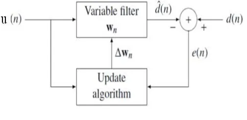
An adaptive discrete filter accepts aninputu(n) and produces an output y(n) due a convolution with the filter weight wn.
A reference wished signal d(n), is compared at the output to obtain an error estimate e(n). This error signal is used to increasingly adjust the filter weight for the next interval of time as shown in fig 1. There are several algorithms used to adjust the weight among them are the LMS (Least Mean Square) and the RLS (Recursive Least Square) algorithms. This work describes the implementation of the RLS algorithm in an FPGA Spartan 3 from Xilinx, using Matlaband System Generator tools due to its faster convergence over other adaptive algorithms.
II. RECURSIVE LEAST SQUARE ALGORITHM
The Recursive least squares (RLS)adaptive filter is an algorithm which recursively finds the filter coefficients that minimize a weighted linear least squarescost function relating to the input signals. This in contrast to other algorithms such as the least mean squares that aim to reduce the mean square error. In the derivation of the RLS, the input signals are considered deterministic, Compared to most of its competitors, the RLS exhibits extremely fast convergence. The RLS algorithm is used in the training of neural network and advanced machine learning algorithms. It uses a rough gradient approximation, and seeks the wished weight vector [3].
This process is used to find the weight vectors for training the ALC (Adaline) [2]. The learning rules can be incorporate to the same device that therefore can be auto adapted as there are presented the wished inputs and outputs. The weight vectors values are changed as every combination input-output is processed. This goes on until the ALC gives the correct outputs. This is a truly training process since there is not necessary to clearly calculate the weight vector value. The input signal is the sum of a desired signal d(n) and interfering noise v(n)
u(n) = d(n) + v(n)
The variable filter has a Finite Impulse Response (FIR) structure. For such structures the impulse response is equal to the filter coefficients. The coefficients for a filter of order p are defined as
The error signal or cost function is the difference between the desired and the estimated signal
The weighted least squares error function C— the cost function we desire to minimize—being a function of e(n) is therefore also dependent on the filter coefficients:
where is the "forgetting factor" which gives exponentially less weight to older error samples. That is it determines how the algorithm treats past data input to the algorithm. The RLS algorithm has infinite memory — all error data is given the same consideration in the total error. In cases where the error value might come from a spurious input data point or points, the forgetting factor lets the RLS algorithm reduce the value of older error data by multiplying the old data by the forgetting factor. When λ = 1, all previous error is considered of equal weight in the
total error. As λ approaches zero, the past errors play a smaller role in the total. The cost function is minimized by
taking the partial derivatives for all entries k of the coefficient vector and setting the results to zero
where is the weighted sample correlation matrix for x(n), and is the equivalent estimate for the cross-correlation between d(n) and x(n), where x(n) is the received signal which is the vector containing the p most recent samples of x(n).
Based on this expression we find the coefficients of the filter which minimize the cost function as
The variable filter updates the filter coefficients at every time instant as
where is a correction factor at time n-1. The adaptive algorithm generates this correction factor based on the input and error signals.
where is the a priori error. Compare this with the a posteriori error; the error calculated after the filter is updated:
The correction factor is given by
Where g(n) is the gain vector given by
This intuitively satisfying result indicates that the correction factor is directly proportional to both the error and the gain
vector, which controls how much sensitivity is desired, through the weighting factor, λ.
III. IMPLEMENTATION IN MATLAB
purpose of taking different samples of the input signal in the time, u(n) n = 1, 2, 3, 4…, some delays are used. Then this signal is multiplied by the error resulting from the difference between the wished signal and the actual one of the filter, to this product it is added the previous weight value to obtain the actual weight value. The filter output results from the product between the input signal u(n) and the actual weight value w(n). This is described in the following expressions:
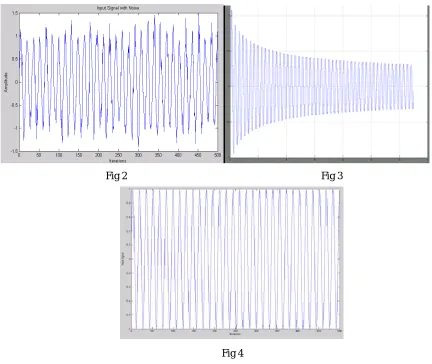
Finally the signal with noise, the output signal and the error signal are viewed as the MATLAB results shown in Fig 2 to 4.
Fig 2. Input Sinusoidal Signal with Noise Fig 3. Output Error Signal Fig 4. Output signal
The algorithm on the similar way is implemented for the audio signals where in the two input signals of the adaptive filters are one being the original audio signal i.e., the desired signal d(n) and the other being the signal corrupted by random noise. The filters adjusts the weights based on the factor specified and as time goes on, it is observed that the
Fig 2 Fig 3
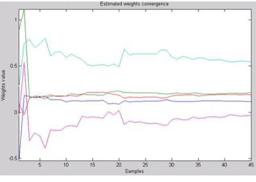
signal at the filter output is close to the wished one and the error signal e(n) is reduced. This due to system stabilization as the error diminishes as time increases. The estimated weight convergence is plotted for various adaptive filters and the one plotted in dark blue for RLS algorithm is seen to have a better and faster convergence as shown in Fig 5.
IV.IMPLEMENTATION AS SIMULINK BLOCK
The Matlab code is the converted to a Simulink block using the AccelDSP software. AccelDSP is a synthesis tool that allows one to transform a MATLAB floating-point design into a hardware module that can be implemented in a Xilinx FPGA. The AccelDSP Synthesis Tool features an easy-to-use Graphical User Interface that controls an integrated environment with other design tools such as MATLAB, Xilinx ISE tools, and other industry- standard HDL simulators and logic synthesizers.
The software initially generates a fixed point from a floating point [10]. The generated floating points are then verified and the RTL is generated for the desired target which is for the family Spartan 3e with xc3s500e for the package fg320 with speed -5 with maximum I/O’s as 232 and frequency as 100MHz and the required number of I/O’s are calculate by the simulator. Finally the RTL is verified for the simulation tool of ISE Simulator with target language as VHDL as to be implemented in FPGA and finally generating the system generator producing the block for the given code and is added as a block in the Simulink library.
V.IMPLEMENTATION IN FPGA
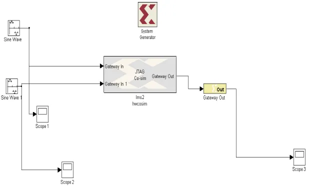
Before loading the software in the FPGA, with the System Generator icon, a block called JTAG is created, this enables the passing of the program to the card through a cable. The JTAG block obtained is tested using the same procedure as that adapted for the Simulink block to check for the output match between the two results.
Fig 8 JTAG Implementation of the Algorithm
VI.CONCLUSION
For obtain the best weight vector in the RLS algorithm, it is necessary to drop or at least to minimize the difference between the wished output and the real one for all the input vectors. The approximation used in this report consists in minimizing the least square error for the input values sets.
Once the RLS algorithm had been implemented, for a particular filter, the algorithm provides a faster convergence and stability although there is high computational complexity its advantage of faster convergence overrides these limitations. The trends at sight are applications oriented based on neural networks field and to the artificial vision field,
oriented to the supervised and not supervised satellite images classification, and of curse all these implemented at a hardware level.
REFERENCES
[1] Joseph Petrone, Adaptive Filter Architectures, Florida, June 2004. [2] B. Widrow, Adaline: Smarter than Sweet,Stanford Today, Autumn 1963.
[3] B. Widrow and S.D. Stearns, Adaptive Signal Processing, Prentice Hall, Englewood Cliffs, NJ, 1985. [4] B. FarhangBoroujeny, Adaptive Filter Theory and applications, Wiley, Singapore, 1999.
[5] B. Widrow and M.A. Lehr, ``Adaptive Neural Networks and their Applications,''International Journal of Intelligent Systems, 8(4):453-507, April 1993.
[6] http://plaza.ufl.edu/badavis/EEL6502_Project_1.html
[7] B. Widrow, J.R. Glover, Jr., J.M. McCool, J. Kaunitz, C.S. Williams, R.H. Hearn, J.R. Zeidler, E. Dong, Jr., and R.C. Goodlin, ``Adaptive Noise Cancelling: Principles and Applications,''Proceedings of the IEEE, 63(12):1692-1716, December 1975.
[8] Tian Lan, Jinlin Zhang, "FPGA Implementation of an Adaptive Noise Canceller," isip, pp.553-558, 2008 International Symposiums on Information Processing, 2008.
[9] C. Shi, R. W. Brodersen, “A Tutorial of Floating-point to Fixed-point Conversion Tool on a BPSK Communication System”, March 27, 2004. [10] Changchun Shi, Floating-point to fixed-point conversion, May, 2004, Ph. D Thesis, Department of EECS, University of California, Berkeley. [11] Garimamalik, Amandeep Singh Sappal, “Adaptive Equalization Algorithms:An Overview”, International Journal of Advanced
ComputerScience and Applications, March 2011.
[12] Jitendra Kumar Das, K. K. Mahapatra, “design of adaptive hearing aid algorithm using booth Wallace tree multiplier”, CSC Journal, December2010.