Flocking Behaviour Simulation : Explanation and
Enhancements in Boid Algorithm
Mohit Sajwan*, Devashish Gosain**, Sagarkumar Surani**
*Masters of Engineering, Department of Computer Science and Engineering,Birla Institute Of Technology, Mesra, Ranchi, Jharkhand 835215, India
**Masters of Technology, Department of Computer Science and Engineering,Birla Institute Of Technology, Mesra, Ranchi, Jharkhand 835215, India
Abstract-Few things in nature is as impressive as how some animals seems to be able to organize themselves into larger groups so effortlessly. By learning more about this fascinating behavior we might be able to apply this knowledge to find new solutions to our own problems. One of the first stepping stones to get to an understanding of flocking behavior is to be able to simulate it. The first flocking-behavior simulation was done on a computer by Craig Reynolds in 1986 he called his simulation program: “Birds”. It’s still to this day to most used model for simulating flocking behavior. This paper attempts to critically examine the algorithm proposed with some modifications and enhancements.
I. BACKGROUND
Animal behavior has always been a source of amazement to mankind. In many areas the abilities of the animals surpasses the abilities of us humans, but with the use of technology we have been able to best the animals in more and more areas. By studying the behavior of animals we have been able to find many interesting solutions animals apply to the problems in their environment. These solutions has inspired many people to think of problems in new ways, sometimes leading to new solutions, often with great results. But few things are more impressive than the way some creatures organize themselves in larger groups: birds, fishes and ants; flocks, shoals and swarms. If we can understand the mechanism of how these organizations emerge, we might be able to use the same mechanics to achieve what we have not achieved before.
II. INTRODUCTION
Flocking is a computer model for the coordinated motion of groups (or flocks) of entities called birds. Flocking represents group movement—as seen in bird flocks and fish schools—as combinations of steering behaviors for individual birds, based on the location and velocities of nearby flock mates. Though individual flocking behaviors (sometimes called conducts) are quite simple, they combine to give birds and flocks interesting overall behaviors, which would be complicated to program explicitly. Flocking is often grouped with Artificial Life algorithms because of its use of emergence: complex global behaviors arise from the interaction of simple local conducts. A crucial part of this complexity is its unpredictability over time; a bird flying in a particular direction may do something different a few moments later. Flocking is useful for games where groups of things, such as soldiers, monsters, or crowds move in complex, coordinated ways. Flocking appears in games
such as Unreal (Epic), Half-Life (Sierra), and Enemy Nations (Windward Studios). [1]
One of the first stepping stones to get to an understanding of flocking behavior is to be able to simulate it. With a simulation we could easily play around with the different parameters and find a variant that suits our needs. The first flocking-behavior simulation was done on a computer by Craig Reynolds in 1986 he called his simulation program: “Birds” [2]. Birds was named after the simple agents in the system which he also called birds. The birds used a set of simple conducts to determine how they would move. The three conducts formulated by Reynolds in his Birds program are still the basis of modern flocking simulation and are widely used to these days. These are the three conducts as they are described by Reynolds on his website [3]:
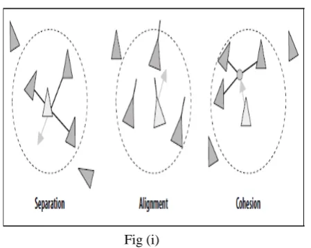
Separation Steer to avoid crowding local flockmates.
Alignment Steer towards the average heading of local flockmates.
Cohesion Steer to move toward the average location of local flockmates.
In 1990 Frank Heppner and Ulf Grenander proposed another model for simulating flocking behavior [4]. Their model also consists largely by the application of three conducts:
Homing each member of the flock tries to stay in the roosting area.
Velocity regulation each member of the flock tries to fly with a certain predefined flight speed - it tries to return to that speed if perturbed.
Interaction if two flockmates are too close to one another, they try to move apart; if they are too distant, they do not influence each other; otherwise they try to move closer together.
One of the primary features of this model (in contrast to Reynolds model) is the inclusion of random disturbances. It simulated this disturbances with a Poisson stochastic process, however one of the weaknesses of this model is that it won’t yield satisfiable results without these disturbances.
In this report we decided to focus on Reynolds model for flocking behavior, for several reasons:
• It is the most widely used of the two.
The three conducts of Reynolds can be graphically depicted as
Fig (i)
The circles in Figure (i) surround the center bird’s local flockmates. Any birds beyond a certain distance of the central bird don’t figure in the conduct-based calculations. A more elaborate notion of neighborhood only considers flockmates surrounding the bird’s current forward direction (Figure (ii)). The extent of neighborhood is governed by an arc on either side of the forward vector. This reduced space more closely reflects how real-world flock members interact.
Fig (ii)
Many other conducts have been proposed over the years, including ones for obstacle avoidance and goal seeking. Reynolds’s web site (http://www.red3d.com/cwr/birds/) contains hundreds of links to relevant information, including flocking in games, virtual reality, computer graphics, robotics, art, and artificial life.
The following section explains the Pseudocode in detail followed by further modifications.
III. THE PSEUDOCODE
The birds program has the following structure: start_simulation() LOOP draw_birds()
mov_birds_to_new_loc()
END LOOP
The start_simulation() procedure puts all the birds at a starting location. Purposely they are placed at random locations off-screen to start with, so that when the
simulation starts they all fly in towards the middle of the screen, rather than suddenly appearing in mid-air.
The draw_birds() procedure simply draws one 'frame' of the animation, with all the birds in their current locations. Note that the boids’ algorithm works just as well in two dimensions as it does in three dimensions.
The procedure we have called mov_ birds_ to_ new_ loc() contains the actual boids algorithm. Note that all it involves simple vector operations on the locations of the birds. Each of the birds’ conducts works independently, so, for each bird, we can calculate how much it will get moved by each of the three conducts, calculating three velocity vectors. Then we can add those three vectors to the bird's current velocity to work out its new velocity. Interpreting the velocity as how far the bird moves per time step we simply add it to the current location, arriving at the following pseudo-code:
PROCEDURE mov_birds_to_new_loc() Vector v1, v2, v3
Bird b
FOR EACH BIRD b
v1 = conduct1 (b) v2 = conduct2 (b) v3 = conduct3 (b)
b.velocity = b.velocity + v1 + v2 + v3 b.location = b.location + b.velocity END
END PROCEDURE
We'll now look at each of these three conducts in turn. The Birds Conducts
Conduct 1: Birds try to fly towards the centre of location of neighboring birds.
The 'center of location' is simply the average location of all the birds. Assume we have N birds, called b1, b2, ..., bN.
Also, the location of a bird b is denoted b.location. Then the 'centre of location' c of all N birds is given by:
c = (b1.location + b2.location + ... + bN.location) / N
(Locations here are vectors, and N is a scalar.)
However, the 'centre of location' is a property of the entire flock; it is not something that would be considered by an individual bird. We prefer to move the bird toward its 'perceived centre', which is the centre of all the other birds, not including itself. Thus, for birdJ (1 <= J <= N), the
perceived centre pcJ is given by:
tloc = (b1.location + b2.location + ... + bJ-1.location
+bJ+1.location + ... + bN.location
)
pcJ = tloc/N-1
Having calculated the perceived centre, we need to work out how to move the bird towards it. To move it 1% of the way towards the centre (this is about the factor we use) this is given by (pcJ - bJ.location) / 100.
Summarizing this in pseudocode: PROCEDURE conduct1 (bird bJ)
Vector pcJ
FOR EACH BIRD b
IF b!= bJ THEN
pcJ = pcJ + b.location
END pcJ = pcJ / N-1
RETURN (pcJ - bJ.location) / 100
END PROCEDURE
Thus we have calculated the first vector offset, v1, for the bird.
Conduct 2: Birds try to keep a small distance away from
other objects (including other birds).
The purpose of this conduct is for birds to make sure they don't collide into each other. We will examine each bird, and if it's within a defined small distance (say 100 units) of another bird move it as far away again as it already is. This is done by subtracting from a vector c the displacement of each bird which is nearby. We initialize c to zero as we want this conduct to give us a vector which when added to the current location moves a bird away from those near it. PROCEDURE conduct2(bird bJ)
Vector c = 0; FOR EACH BIRD b IF b != bJ THEN
IF |b.location - bJ.location| < 100
THEN
c = c - (b.location - bJ.location)
END IF
END IF
END RETURN c
END PROCEDURE
It may seem odd that we choose to simply double the distance from nearby birds, as it means that birds which are very close are not immediately "repelled". Remember that if two birds are near each other, this conduct will be applied to both of them. They will be slightly steered away from each other, and at the next time step if they are still near each other they will be pushed further apart. Hence, the resultant repulsion takes the form of a smooth acceleration. It is a good idea to maintain a principle of ensuring smooth motion. If two birds are very close to each other it's probably because they have been flying very quickly towards each other, considering that their previous motion has also been restrained by this conduct. Suddenly jerking them away from each other, such that they each have their motion reversed, would appear unnatural, as if they bounced off each other's invisible force fields. Instead, we have them slow down and accelerate away from each other until they are far enough apart for our liking.
Conduct 3: Birds try to match velocity with near birds.
This is similar to Conduct 1, however instead of averaging the locations of the other birds we average the velocities. We calculate a 'perceived velocity', pvJ, then add a small
portion (about fourth) to the bird's current velocity.
PROCEDURE conduct3(bird bJ)
Vector pvJ
FOR EACH BIRD b IF b != bJ THEN
pvJ = pvJ + b.velocity
END IF
END
pvJ = pvJ / N-1
RETURN (pvJ - bJ.velocity) / 4
END PROCEDURE
IV. FURTHER IMPROVEMENTS
The three birds conducts sufficiently demonstrate a complex emergent flocking behaviour. They are all that is required to simulate a distributed, leaderless flocking behaviour.
However in order to make other aspects of the behaviour more life-like, extra conducts and limitations can be implemented.
These conducts will simply be called in the mov_birds_to_new_loc() procedure as follows:
PROCEDURE mov_birds_to_new_loc() Vector v1, v2, v3, v4, ...
FOR EACH BIRD b v1 = conduct1(b) v2 = conduct2(b) v3 = conduct3(b) v4 = conduct4(b)
… . …
b.velocity = b.velocity + v1 + v2 + v3+ v4 + ... b.location = b.location + b.velocity
END
END PROCEDURE
Hence each of the following conducts is implemented as a new procedure returning a vector to be added to a bird's velocity.
V. GOAL SETTING
Reynolds uses goal setting to steer a flock down a set path or in a general direction, as required to ensure generally predictable motion for use in computer animations and film work. We have not used such goal setting in our simulations, however here are some example implementations:
A. ACTION OF A STRONG WIND OR CURRENT For example, to simulate fish schooling in a moving river or birds flying through a strong breeze.
PROCEDURE strong_wind(Bird b)
Vector wind
RETURN wind
END PROCEDURE
This function returns the same value independent of the bird or fish being examined; hence the entire flock will have the same push due to the wind.
realistically mill around the gate and slowly trickle through it.
PROCEDURE tend_to_place(Bird b)
Vector place
RETURN (place - b.location) / 100 END PROCEDURE
Note that this conduct moves the bird 1% of the way towards the goal at each step. Especially for distant goals, one may want to limit the magnitude of the returned vector.
C. LIMITING THE SPEED
We find it a good idea to limit the magnitude of the birds' velocities, this way they don't go too fast. Without such limitations, their speed will actually fluctuate with a flocking-like tendency, and it is possible for them to momentarily go very fast. We assume that real animals can't go arbitrarily fast, and so we limit the birds' speed. (Note that we are using the physical definitions of velocity and speed here; velocity is a vector and thus has both magnitude and direction, whereas speed is a scalar and is equal to the magnitude of the velocity).
For a limiting speed vlim:
PROCEDURE limit_velocity(Bird b) Integer vlim
Vector v
IF |b.velocity| > vlim THEN
b.velocity = (b.velocity / |b.velocity|)* vlim END IF
END PROCEDURE
This procedure creates a unit vector by dividing b.velocity by its magnitude, then multiplies this unit vector by vlim. The resulting velocity vector has the same direction as the original velocity but with magnitude vlim.
Note that this procedure operates directly on b.velocity, rather than returning an offset vector. It is not used like the other conducts; rather, this procedure is called after all the other conducts have been applied and before calculating the new location, i.e. Within the procedure move_all_birds_to_new_locations:
b.velocity = b.velocity + v1 + v2 + v3 + ... limit_velocity(b)
b.location = b.location + b.velocity
D. BOUNDING THE LOCATION
In order to keep the flock within a certain area (e.g. to keep them on-screen), rather than unrealistically placing them within some confines and thus bouncing off invisible walls, we implement a conduct which encourages them to stay within rough boundaries. That way they can fly out of them, but then slowly turn back, avoiding any harsh motions.
PROCEDURE bound_location(Bird b)
Integer Xmin, Xmax, Ymin, Ymax, Zmin, Zmax
Vector v
IF b.location.x < Xmin THEN
v.x = 10
ELSE IF b.location.x > Xmax THEN
v.x = -10
END IF
IF b.location.y < Ymin THEN
v.y = 10
ELSE IF b.location.y > Ymax THEN
v.y = -10
END IF
IF b.location.z < Zmin THEN v.z = 10
ELSE IF b.location.z > Zmax THEN v.z = -10
END IF
RETURN v
END PROCEDURE
Note: the value 10 is an arbitrary amount to encourage them to fly in a particular direction.
E. PERCHING
The desired behaviour here has the birds occasionally landing and staying on the ground for a brief period of time before returning to the flock. This is accomplished by simply holding the bird on the ground for a brief period (of random length) whenever it gets to ground level, and then letting it go.
When checking the bounds, we test if the bird is at or below ground level, and if so we make it perch. We introduce the Boolean b.perching for each bird b. In addition, we introduce a timer b.perch_timer which determines how long the bird will perch for. We make this a random time, assuming we are simulating the bird eating or resting.
Thus, within the bound_location procedure, we add the following lines:
Integer GroundLevel
...
IF b.location.y < GroundLevel THEN b.location.y = GroundLevel b.perching = True
END IF
It is held on the ground by simply not applying the birds’ conducts to its behaviour (obviously, as we don't want it to move). Thus, before attempting to apply the conducts we check if the bird is perching, and if so we decrement the timer b.perch_timer and skip the rest of the loop. If the bird has finished perching then we reset the b.perching flag to allow it to return to the flock.
PROCEDURE mov_birds_to_new_loc()
Vector v1, v2, v3, ... Bird b
FOR EACH BIRD b
IF b.perching THEN
IF b.perch_timer > 0 THEN b.perch_timer = b.perch_timer - 1 NEXT
ELSE b.perching = FALSE
END IF
v1 = conduct1(b) v2 = conduct2(b) v3 = conduct3(b)
... b.velocity = b.velocity + v1 + v2 + v3 + ... ... b.location = b.location + b.velocity END
END PROCEDURE
Note that nothing else needs to be done to simulate the perching behaviour. As soon as we re-apply the birds conducts this bird will fly directly towards the flock and continue on as normal.
VI. ANTI-FLOCKING BEHAVIOUR
During the course of a simulation, one may want to break up the flock for various reasons. For example the introduction of a predator may cause the flock to scatter in all directions.
A. SCATTERING THE FLOCK
Here we simply want the flock to disperse; they are not necessarily moving away from any particular object, we just want to break the cohesion (for example, the flock is startled by a loud noise). Thus we actually want to negate part of the influence of the birds conducts.
Of the three conducts, it turns out we only want to negate the first one (moving towards the centre of mass of neighbors) – i.e. We want to make the birds move away from the centre of mass. As for the other conducts: negating the second conduct (avoiding nearby objects) will simply cause the birds to actively run into each other, and negating the third conduct (matching velocity with nearby birds) will introduce a semi-chaotic oscillation.
It is a good idea to use non-constant multipliers for each of the conducts, allowing us to vary the influence of each conduct over the course of the simulation. If we put these
multipliers in the move_all_birds_to_new_locations procedure, the new
definition of this procedure will be : PROCEDURE mov_birds_to_new_loc ()
Vector v1, v2, v3,... Integer m1, m2, m3,... Bird b
FOR EACH BIRD b ...
v1 = m1 * conduct1 (b) v2 = m2 * conduct2 (b) v3 = m3 * conduct3 (b) ...
b.velocity = b.velocity + v1 + v2 + v3 + ... ...
b.location = b.location + b.velocity END
END PROCEDURE
Then, during the course of the simulation, simply make m1 negative to scatter the flock. Setting m1 to a
positive value again will cause the flock to spontaneously re-form.
B. TENDENCY AWAY FROM A PARTICULAR PLACE
If, on the other hand, we want the flock to continue the flocking behaviour but to move away from a particular place or object (such as a predator), then we need to move each bird individually away from that point. The calculation required is identical to that of moving towards a particular place, implemented above as tend_to_place; all that is required is a negative multiplier:
Vector v
Integer m
Bird b
...
v = -m * tend_to_place(b)
So we see that each of the extra routines are very simple to implement, as are the initial conducts. We achieve complex, life-like behaviour by combining all of them together. By varying the influence of each conduct over time we can change the behaviour of the flock to respond to events in the environment such as sounds, currents and predators.
VII. AUXILIARY FUNCTIONS
It is handy to set up a set of Vector manipulation routines first to do addition, subtraction and scalar multiplication and division. For example, all the additions and subtractions in the above pseudocode are vector operations, so for example the line:
pcJ = pcJ + b.location
will end up looking something like:
pcJ = Vector_Add(pcJ, b.location)
where, Vector_Add is a procedure defined thus: PROCEDURE Vector_Add(Vector v1, Vector v2)
Vector v
v.x = v1.x + v2.x v.y = v1.y + v2.y v.z = v1.z + v2.z
RETURN v
END PROCEDURE and the line:
pcJ = pcJ / N-1
will be something like:
pcJ = Vector_Div(pcJ, N-1)
where Vector_Div is a scalar division:
PROCEDURE Vector_Div(Vector v1, Integer A)
Vector v
v.x = v1.x / A v.y = v1.y / A v.z = v1.z / A
RETURN v
END PROCEDURE
VIII. APPLICATIONS
In Cologne, Germany, two biologists from the University of Leeds demonstrated a flock like behavior in humans. The group of people exhibited a very similar behavioral pattern to that of a flock, where if 5% of the flock would change direction the others would follow suit. When one person was designated as a predator and everyone else was to avoid him, the flock behaved very much like a school of fish.
Flocking has also been considered as a means of controlling the behavior of Unmanned Air Vehicles (UAVs).
Flocking is a common technology in screensavers, and has found its use in animation. Flocking has been used in many films to generate crowds which move more realistically. Tim Burton's Batman Returns (1992) featured flocking bats, and Disney's The Lion King (1994) included a wildebeest stampede.
Flocking behaviour has been used for other interesting applications. It has been applied to automatically program
Internet multi-channel radio stations. It has also been used for visualizing information and for optimization tasks. [5,6]
IX. CONCLUSION
There has been significant applications, of above mentioned Boid’s algorithm. There can be more possible conducts and constraints in Boid’s Algorithm. Depending on the need and application of this algorithm in different domains, there can be multiple conducts implemented using the specific domain knowledge.
REFERENCES
[1] Killer Programing in Java ( chapter 22), Andrew Davison [2] Craig W. Reynolds. Flocks, herds, and schools: A distributed
behavioral model. In Computer Graphics, pages 25–34, 1987. [3] Craig W. Reynolds. Boids, Background and Update.
http://www.red3d.com/cwr/boids/, 2007.
[4] F. Heppner and U. Grenander. A stochastic nonlinear model for coordinatedbird flocks. 1990.