Article
1
Short-Term Forecast of Wind Speed through
2
Mathematical Models
3
Moniki Ferreira 1, Alexandre Santos 2 and Paulo Lucio 3,*
4
1 Postgraduate Program in Climate Sciences, Department of Atmospheric Sciences and Climate, Federal
5
University of Rio Grande do Norte, Brazil; [email protected]
6
2 Applied Research Unit, Centre for Gas Technology and Renewable Energy (UNPA/CTGAS-ER), Natal,
7
Brazil; [email protected]
8
3 Department of Atmospheric Sciences and Climate, Federal University of Rio Grande do Norte, Brazil
9
* Correspondence: [email protected]; Tel.: +55-84-999536920
10
11
Abstract: The predictability of wind information in a given location is essential for the evaluation of
12
a wind power project. Predicting wind speed accurately improves the planning of wind power
13
generation, reducing costs and improving the use of resources. This paper seeks to predict the
14
mean hourly wind speed in anemometric towers (at a height of 50 meters) at two locations: a
15
coastal region and one with complex terrain characteristics. To this end, the Holt-Winters (HW),
16
Artificial Neural Networks (ANN) and Hybrid time-series models were used. Observational data
17
evaluated by the Modern-Era Retrospective analysis for Research and Applications-Version 2
18
(MERRA-2) reanalysis at the same height of the towers. The results show that the hybrid model had
19
a better performance in relation to the others, including when compared to the evaluation with
20
MERRA-2. For example, in terms of statistical residuals, RMSE and MAE were 0.91 and 0.62 m/s,
21
respectively. As such, the hybrid models are a good method to forecast wind speed data for wind
22
generation.
23
Keywords: wind speed; ANN model; hybrid model
24
25
1. Introduction
26
In recent years researches from several nations have warmed of the possible consequences of
27
global warming across the planet, encouraging the use of font’s renewable energy resources, for
28
examples wind energy, is one of the strategies used to mitigate greenhouse gases from human
29
activities in the atmosphere [1,2]. The wind energy capacity installed at the end of 2016 in Brazil was
30
approximately of 11 GW, with estimate for 2020 will have around 18 GW of installed wind energy
31
capacity, which will contribute to the country’s energy security [3].
32
Most research in the field of wind is being applied to wind power (conversion of kinetic energy
33
into electrical energy) for the planning and development of wind farms (set of wind turbines) [4].
34
Wind power is a renewable and clean source of energy, available with variable behavior in each part
35
of the world because of the different climatic and geographical characteristics of each region [4].
36
Wind is caused by solar energy hitting the earth's surface and atmosphere, which together with the
37
planetary rotation results in an uneven heating of the atmosphere and, consequently, differentials in
38
atmospheric pressures [5].
39
The predictability of wind information at a particular location is essential for the assessment of
40
a wind energy exploitation project. In this context, accurately predicting the wind speed means
41
improving the planning of wind power generating facilities, thus reducing mistakes and economic
42
costs [4].
43
The development of Artificial Intelligence (AI) with various methods for forecast wind speed
44
was also created. The methods were: Artificial Neural Network (ANN); adaptive neuro-fuzzy
45
inference system (ANFIS); fuzz logic methods; support vector machine (SVM), –support vector
46
machine and neuro-fuzzy network. Accurate forecasts of short-term wind speed and
47
generation of energy are essential for the effective operation of a wind farm. The short-term forecast
48
of wind speed is also critical to the operation of wind turbines so that dynamic controls can be
49
accomplished to increase the energy conversion efficiency [6]. Reference [6] proposed a method
50
using improved radial basis function neural network-based model with an error feedback scheme
51
(IRBFNN-EF) for forecasting short-term wind speed and power of a wind farm. Results showed that
52
the proposed model IRBFNN-EF leads to better accuracy for forecasting wind speed and wind
53
power, compared with those obtained by four other artificial neural network-based forecasting
54
methods. Reference [7] compared the performances of autoregressive integrated moving average
55
(ARIMA), Auto-Regressive Integrated Moving Average with Exogenous (ARIMAX), ANN and
56
hybrids (ARIMA-ANN and ARIMAX-ANN) models in wind speed predictions in the Brazilian
57
Northeast region (Fortaleza, Natal and Paraiba). The hybrid model proposed in this study was
58
efficient in reducing statistical errors, especially when compared to traditional models (ARIMA,
59
ARIMAX and ANN), with lowest percentage error between the observed and the adjusted series, of
60
only about 8%.
61
Some recent studies have been developed about the short-term predictability of wind speeds
62
with the use of dynamic, mathematical and statistical tools using Numerical Weather Prediction
63
(NWP) [8,9], stochastic [10] and hybrid [3,7,11] models. Reference [12] investigated the prediction of
64
hourly wind speeds at 30 m above ground with the atmospheric model WRF (Weather Research
65
Forecasting) for the State of Alagoas-Brazil. The difficulties encountered in this study included: (i)
66
forecasting extreme values; (ii) minimums and maximums and (iii) forecasts in rainy periods. In the
67
study, the same difficulties were also found for the forecast of wind speed for wind power
68
generation through the outputs of mesoscale weather models in the Northeast Region of Brazil
69
(NEB). Other feasible wind speed studies can be found in [13], which proposed methods to fill gaps
70
in wind speed data - located in Rio Grande do Norte (Northeast Region of Brazil) - reducing the
71
propagation of residuals in the results. Reference [10] studied and developed forecasting models, of
72
short-term wind speed. The methods of exponential smoothing, in particular the method
73
Holt-Winters (stochastic model) and its variations, are suitable in this context because of its high
74
adaptability and robustness for apply the methodology in the wind speed data anemometric tower
75
in city of São João do Cariri (State of Paraíba-Brazil), which will be compared with models:
76
persistence and neuro-fuzz (ANFIS). Results showed that the proposed Holt-Winters additive model
77
were satisfactory, compared with those obtained by two tested models (persistence and
78
neuro-fuzzy) in the same wind speed time-series for short-term forecasting. Reference [14] proposed
79
a hybrid model that consists of the EWT (Empirical Wavelet Transform), CSA (Coupled Simulated
80
Annealing) and LSSVM (Least Square Support Vector Machine) for enhancing the accuracy of
81
short-term wind speed forecasting. Results suggest that the developed forecasting method better
82
compared with those other models, which indicates that the hybrid model exhibits stronger
83
forecasting ability.
84
The spatial and temporal variability of the wind is difficult to simulate with precision. This is a
85
result of the heterogeneity of regions regarding such factors as: surface roughness, vegetation
86
variability and soil use and occupation [15]. In addition, several meteorological and climatic
87
phenomena may influence the atmospheric dynamics of the NEB region [16]. Systematic errors occur
88
with a certain frequency in the simulations of dynamic models, which means models with greater
89
accuracy need to be developed for the short-term wind speed forecasting of a particular site [17].
90
Reference [18] presented a system consists of a numerical weather prediction model and ANN of a
91
novel day-ahead wind power forecasting in China, in addition Kalman filter integrated to reduce the
92
systematic errors in wind speed from WRF and enhance the forecasting accuracy. Results showed
93
the Normalized Root Mean Square Error (NRMSE) has a month average value of 16.47%, which is an
94
acceptable error margin. To reduce these systematic errors in the outputs of an NWP, lots of
95
This type of statistical relationship could be modeled by various methods for wind speed variable,
97
including the ANNs [6,19,20], Kalman filter [18], ARIMA [7] and hybrid method [11,14,21,22].
98
Wind energy is considered to be technically feasible when its power density is greater than or
99
equal to 500 W/m2, for a height equal to or exceeding 50 m above the ground, which requires a
100
minimum wind speed between 7-8 m/s. Only 13% of the earth's surface has average wind speeds
101
greater than or equal to 7 m/s at the height of 50 m above ground [23,24].
102
In this context, this study seeks to present different methodologies that may assist in this
103
regard, while at the same time proposing a model that has less error in relation to the dynamic
104
models (more systematic errors) in the short term wind speed forecasts at a height of 50 meters
105
above ground in two localities with different geographic and climatic characteristics in the NEB
106
region. One of these locations can be found in the heartland of the continent with a complex terrain
107
(Anemometric Tower 1 - TA01) and the other is located in the coastal region with a flat terrain
108
(Anemometric Tower 2 - TA02). The objective of this study is to present mathematical and statistical
109
models as suitable tools for the forecasting of wind speed variability during the diurnal cycle (24
110
hours), which could be used as an early warning system for wind power generation in the same time
111
scale.
112
The content of this paper is organized as follows: Section 1 reviews the current status of wind
113
speed variable for short-term forecasting with applicability in wind power; Section 2 describes the
114
regions of study, dataset and theory of the Holt-Winters, ANN, hybrid models and its working
115
principles; Section 3 analyzes the errors of the short-term predicted results; Section 4 description of
116
discussion to explore the significance of the study; Section 5 the conclusions of the study.
117
2. Materials and Methods
118
In this section we comment on the data of the regions of study, as well as on the forecasting
119
models. The measurement data is used to identify the accuracy of the forecast calculated by the
120
mathematical models, by comparing the output of each model to the time series observed. All the
121
calculations produced in this paper as well as the graphical part were executed with the software R
122
(https://www.r-project.org/).
123
2.1. Region of study and dataset
124
The measured wind data were obtained from the TA-01 and TA-02 towers, the first located in
125
Belo Jardim - state of Pernambuco, and the second in Camocim - state of Ceará, all located in the
126
Northeast of Brazil, as shown Figure 1. The Belo Jardim data were obtained through the Sistema de
127
Organização Nacional de dados Ambientais (System for the National Organization of
128
Environmental Data, SONDA, http://sonda.ccst.inpe.br/) and the Camocim data through the
129
Infrastructure department of the state of Ceará (SEINFRA/CE, www.seinfra.ce.gov.br/).
130
The anemometric sensors were installed at heights of 25 and 50 meters from the ground, taking
131
measurements every 10 minutes, within the period from October 01 to December 31, 2004, selected
132
for this study in both locations. The wind speed and direction sensor of the TA-01 tower is the Wind
133
Monitor-MA model 05106 (R. M. Young Company) - it takes measurements of horizontal speeds
134
between 0 to 60 m/s and resists gusts of up to 100 m/s. For the TA-02 tower, the data was recorded
135
with a computerized anemometer; model NRG 9200Plus, manufactured by NRG Systems Inc. The
136
temporal series were integrated in an interval of 1 hour at a height of 50 m above ground level - agl
137
(TA-01 and TA-02) to validate the models evaluated in this study.
138
Table 1 presents the local characteristics and the geographical coordinates of the used wind
139
towers.
140
142
Figure 1. Location of each anemometric tower (TA) used in the presented study in Northeast Brazil.
143
Table 1. Local characteristics and geographical location of the wind towers.
144
City/State Altitude (m) Terrain Vegetation Geographic coordinates
Belo Jardim/PE 718 Plateau Caatinga 8°22’S/36°25’W
Camocim/CE 8 Lowland Caatinga 2°51’56,7°S/40°53’09,2°W
2.2. Methods
145
The forecasts for 24 hours were made with the Holt-Winters, Artificial Neural Networks (ANN)
146
and hybrid models, applying them to the temporal series of the TA-01 and TA-02 towers with the
147
use of the R software. The forecasting methodology consisted in making a division in the series in
148
three steps: (i) the first step used 30 days of data observed in the period from October 01 to 30, 2004,
149
to predict the daily wind speed cycle for the day of October 31, 2004; (ii) The second step used 60
150
days of data observed in the period from October 01 to November 29, 2004, to predict the day of
151
November 30, 2004; and (iii) the third and last step used 90 days of data observed in the period from
152
October 01 to December 29, 2004, to forecast the day of December 30, 2004.
153
There are numerous techniques to forecast wind speeds, such as the NWP methods, statistical
154
methods, ANN and hybrid approaches. The NWP methods may be the most accurate technique for
155
forecasting in the short term. In general, however, statistical methods, ANNs or hybrid approaches
156
have smaller errors in short term forecasts [22].
157
2.2.1. Holt-Winters Model
158
In the year of 1957, Holt expanded the simple exponential smoothing model to deal with the
159
data that showed a linear tendency, thus making predictions that were more accurate than those
160
performed [25]. In year 1960, Winters extended the Holt model, which included a new equation that
161
Holt-Winters is one of the most used methods for the prediction of meteorological variables due
163
to its simplicity, low operating costs, good accuracy and ability to make automatic adjustments and
164
quick changes to the temporal series. This model has the following smoothing coefficients: level,
165
linear trend, seasonal factor and an unpredictable residual element called random error. The
166
exponential adjustment method, also called "exponential smoothing", is used for the estimation of
167
these factors. The name "smoothing" comes from the fact that after its reduction to structural
168
components, a series will have a smaller number of abrupt variations, revealing a smoother
169
behavior. The term "exponential" is used because the smoothing processes involve the weighted
170
arithmetic mean, where the weights decrease exponentially as you progress into the past [10].
171
The prediction equations are allocated in two ways: additively or multiplicatively, according to
172
the nature of the series. To calculate the forecasts of future values of a series, the level and the trend
173
of the series in the current period have to be estimated, just as the seasonal factor values
174
corresponding to the last period of seasonality. These estimates are performed through the following
175
equations:
176
177
Additive Seasonality – The equation referring to the exponential smoothing method with
178
seasonality and linear tendency, with seasonal component being treated in an additive way, is
179
represented as follows:
180
181
(1)
where: is level of the series, whose unit in this particular work is of m/s, shows how the
182
expected time series evolves over time; is tendency, unit here is m/s, this relates to the fact that
183
the predicted time series can have increasing or decreasing motions in different time intervals; is
184
seasonal component, represented here by m/s, which is related to the fact that the expected time
185
series has cyclical patterns of variation that repeat at relatively constant time intervals, is forecast
186
for period and is seasonal period with = 1,2,3,…,n (horizontal forecast).
187
where , and are given by:
188
(2)
189
(3)
190
(4)
Multiplicative Seasonality: – Is similar to the Holt-Winters additive. Holt-Winters Multiplicative
191
method also calculates exponentially smoothed values for level, trend, and seasonal adjustment to
192
the forecast. This method is best for data with trend and with seasonality that increases over time. It
193
results in a curved forecast that reproduces the seasonal changes in the data. The multiplicative
194
Holt-Winters prediction function is:
195
where , and are given by:
196
(6)
197
(7)
198
(8)
where , and are damping constants. At the end of each period , the estimate of the "step"
199
(trend) and the seasonal component are given by and , respectively. The level component, on
200
the other hand, is denoted by .
201
The additive Holt-Winters model was used in the Camocim/CE data for the temporal series of
202
30, 60 and 90 days and the Belo Jardim/PE data for the series of 30 and 60 days. For the Belo Jardim
203
data set with 90 days, therefore, the multiplicative Holt-Winters model was used, since the additive
204
prediction produced negative values.
205
2.2.2. Artificial Neural Network model
206
Artificial Neural Networks (ANNs) are computational models based on the neural structure of
207
intelligent organisms [7]. Their behavior emerges from the interactions between processing units,
208
which compute certain mathematical (usually non-linear) functions. These processing neurons can
209
be distributed in one or more layers and are linked by a large number of connections, which store the
210
knowledge in the model and weigh each input received over the network.
211
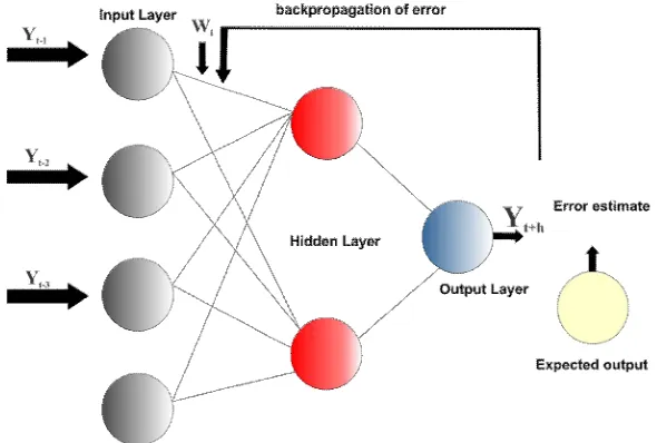
An ANN can be thought of as a network of "neurons" organized in layers. The predictors (or
212
inputs) form the bottom layer, and the forecasts (or outputs) form the top layer. There may be
213
intermediate layers that contain "hidden neurons". The predictors (or inputs ) form the lower
214
layer, and the predictions (or outputs ) form the upper layer. There may be intermediate layers
215
containing hidden neurons [7]. Figure 2 shows an example of an ANN structure with 4 inputs and 1
216
hidden layer. The coefficients related to the predictors are called "weights" and commonly
217
represented by . The weights are selected through a "learning algorithm." This study used the
218
backpropagation algorithm, which is based on the backpropagation of errors to adjust the weights of
219
the intermediate layers, which minimizes the error between the predicted and observed temporal
220
series.
221
223
Figure 2. Example of an ANN structure with 4 inputs layers, 1 hidden layer and 1 output layer.
224
225
226
In terms of use of the ANN by software R, the forecast package also allows for this possibility
227
through the use of the function nnetar() [27]. This study used R's forecast package based on the
228
nnetar() function, which in turn is symbolized by notation , where represents
229
lagged inputs (the quantity of inputs), for example, , , ,..., , , , ,
230
refers to seasonal data, represents the number of neurons in the hidden layer and refers to
231
seasonal data. This function model based on observed wind speed data, if the values
232
of and are not specified, they are automatically selected [3]. For example, NNAR(9,1,4)24 model
233
has inputs , , ,..., and , and four neurons in the hidden layer.
234
The number of network to fit with different random starting weights was equivalent to 20 and
235
is based on the backpropagation learning algorithm for dynamic processing. These are then
236
averaged when producing forecasts.
237
2.2.3 Hybrid model
238
The hybrid model used the hybridModel( ) function of R's forecastHybrid package, with
239
multiple adjustments of the individual models to generate ensemble forecasts. Where is a
240
numeric vector or time series (this work was wind speed time series) and models (combination of
241
model types) by default, the models forecasts generated are from the auto.arima(), ets(), thetam(),
242
nnetar(), stlm(), and tbats() functions, can be combined with equal weights, weights based on
243
in-sample errors [28]. Cross validation for time series data and user-supplied models and forecasting
244
functions is also supported to evaluate model accuracy.
245
The default setting of this package, which works well in most cases, allows for the combination
246
of two to five models through the following arguments:
247
n.args: adjusts a univariate neural network model using the nnetar() function by forecast
248
package [27];
249
a.args: fit best ARIMA model to univariate time series using the auto.arima() function by
250
forecast package. The function conducts a search over possible model within the order
251
constraints provided [27].
252
s.args: is based on the stlm model, which combines the forecast with the adjusted seasonal
253
decomposition, and models the seasonally adjusted data using the model passed or
255
specified using method. It returns an object that includes the original STL decomposition
256
and a time series model fitted to the seasonally adjusted data [27].;
257
t.args: the tbats() function couples the exponential smoothing model with the Box-Cox
258
transformation, ARMA and the seasonal and trend components [28].
259
e.args: Exponential smoothing state space model. Based on the classification of methods as
260
described in Hyndman et al [29]. The only required argument for ets() is the time series [27].
261
The model is chosen automatically if not specified.
262
263
In this work, three "nst" models were adjusted for wind speed forecasting short-term, which
264
were coupled with the arguments: n.args, s.args and t.args. After adjustment of the models by
265
hybridModel() function used the forecast() function with (horizontal forecast) equal to 24 (24 hours)
266
for short-tem forecast of wind speed at each time series proposed in this study.
267
268
269
270
2.2.4. Modern-Era Retrospective analysis for Research and Applications-Version 2 reanalysis dataset
271
The MERRA-2 reanalysis is generated by combining the data assimilation techniques of the
272
models that use dynamic numerical prediction models with the data observed by the global
273
meteorological observation network. The MERRA-2 reanalysis was introduced in the study to
274
evaluate its results in relation to the data observed by the wind towers and predicted by the
275
statistical and mathematical models proposed in this study. The MERRA-2 reanalysis is a
276
freely-available product through the MDISC (Modeling and Assimilation Data and Information
277
Services Center) portal and it is an update to the MERRA project [30].
278
The wind speed data at 50 m agl of MERRA-2 were obtained for the period from October 01 to
279
December 31, 2004 to compare with predicted data from the mathematical and statistical models and
280
observed data (TA-01 and TA-02).
281
2.3. Evaluation of the Models
282
The evaluation of the performance of the forecasting techniques was done through the Pearson
283
correlation coefficient (r), the Mean Absolute Error (MAE) and the Root Mean Square Error (RMSE)
284
[31].
285
2.3.1. Pearson Correlation Coefficient
286
The Pearson Correlation Coefficient is calculated mathematically thus:
287
288
(9)
where:
289
is number of paired values considered;
291
is prediction value (wind speed - m/s);
292
is mean of prediction value;
293
is observed value (wind speed – m/s);
294
is mean of observed value.
295
296
The magnitude of the Pearson correlation coefficient ranges between the values of -1 and 1. This
297
magnitude measures the "intensity" of the relationship between two variables. As such, a coefficient
298
equal to 0.6 has a greater degree of linear dependence than one equal to 0.3. A coefficient with the
299
value of zero indicates the total absence of a linear relationship between the variables and
300
coefficients with the values 1 and -1 suggest a perfect linear dependence. It is therefore used to
301
measure the correlation between the observed and modeled data in order to obtain the degree of
302
linear relationship between both.
303
2.3.2. Mean Absolute Error
304
To evaluate the degree of dispersion between modeled and observed values, they are
305
used as indexes that provide the performance of the model in relation to the observation. The closer
306
the value is to zero, the greater the accuracy of the model and, consequently, the lower its error. The
307
mean absolute error is a measure of the forecasting skill between the observed and predicted series.
308
It is given as a module and is represented mathematically by:
309
(10)
2.3.3. Root Mean Square Error
310
The RMSE was another error index used. It represents the difference between the prediction
311
and the observed value , presenting error values in the same dimensions as the analyzed
312
variable (which in this case is m/s). It can be mathematically defined by:
313
(11)
3. Results
3.1. Available Observational data
316
317
These placed of study have anemometric towers in Camocim-Ceará and Belo
318
Jardim-Pernambuco, located in Brazil. Figure 1 shows the topography of Camocim (coastal region)
319
and Belo Jardim (complex topography) and the location of the study site. The data set used in paper
320
was collected form an anemometer tower, which measuring height is 50 m agl. The available data
321
are from 00:00, 01/10/2004 to 23:50, 31/12/2004, with a time interval of 10 minutes (Figures 3 and 5).
322
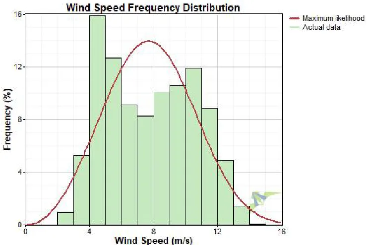
Tables 2 and 3 presented the basic statistical description of the available data. Figures 4 and 6
323
displays the frequencies distributions of the available data and the probability distribution function
324
by the two-parameter Weibull distribution and , where are of shape and scale parameters,
325
respectively. Applying the maximum likelihood method (ML), the shape and scale parameters are
326
3.702/6.406 m/s and 3.096/11.337 m/s for TA-01 and TA-02, respectively.
327
328
329
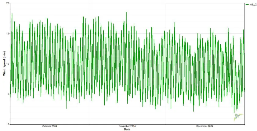
Figure 3. Time series of wind speed (interval of 10 minutes) measurements by the anemometer at a height
330
of 50 m agl of the TA-01 for the period from 01/10/2004 to 31/12/2004.
331
Table 2. Statistical description of wind speed for the 3 months sampling period of the available data
332
of Belo Jardim (TA-01).
333
Possible Data Points
Valid Data Points
Recovery Rate (%)
Mean (m/s)
Median (m/s)
Minimum (m/s)
Maximum (m/s)
Standard Deviation
13.249 13.249 100 5.780 5.730 0.250 11.650 1.725
336
337
Figure 4. Histogram derived from the estimate Weibull probability density function (PDF) by maximum
338
likelihood method compared with the histogram of the wind speed data (bar diagram) for the period of 3
339
months at wind site Belo Jardim (TA-01). Applying the ML method, the shape and scale parameters are
340
and .
341
342
Figure 5. Time series of wind speed (interval of 10 minutes) measurements by the anemometer at a height
343
of 50 m agl of the TA-02 (Camocim) for the period from 01/10/2004 to 31/12/2004.
344
345
Table 3. Statistical description of wind speed for the 3 months sampling period of the available data
346
of Camocim (TA-02).
347
Possible Data Points
Valid Data Points
Recovery Rate (%)
Mean (m/s)
Median (m/s)
Minimum (m/s)
Maximum (m/s)
Standard Deviation
13.249 13.249 100 7.771 7.747 1.789 14.579 2.773
349
350
Figure 6. Histogram derived from the estimate Weibull probability density function (PDF) by maximum
351
likelihood method compared with the histogram of the wind speed data (bar diagram) for the period of 3
352
months at wind site Camocim (TA-02). Applying the ML method, the shape and scale parameters are
353
and .
354
3.2. Quantitative and Qualitative Analysis of the 24-Hour Forecast
355
3.2.1. Based on 30 days of data
356
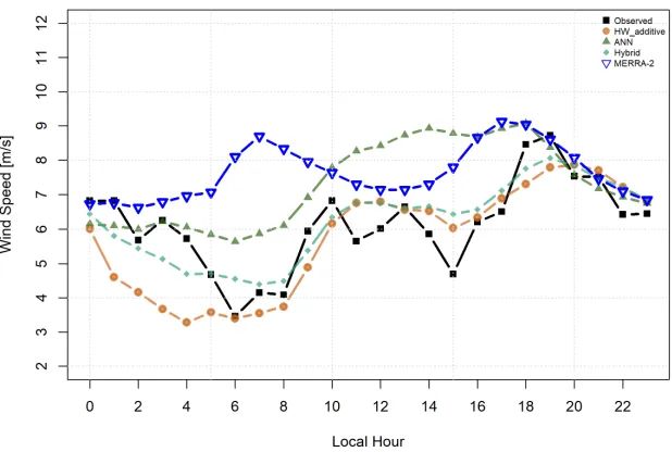
Figures 7 and 8 present the forecast for the day 31/10/2004 using 30 days of observations
357
(01/10/2004 to 30/10/2004) for the locations of the TA-01 and TA-02 towers, respectively. The
358
Holt-Winters, Artificial Neural Network and Hybrid models and the MERRA-2 reanalysis are
359
shown in Figures 3 and 4 along with the observations.
360
For the TA-01 tower (Figure 7), it is possible to identify that the models follow the diurnal
361
behavior of the observations, but they do not adequately capture the extreme values for minimum
362
variation at certain times, showing a smoother pattern. The MERRA-2 reanalysis overestimates the
363
observations between the 2h to 19h range and at other times it fits with the observations. The ANN
364
model underestimates the first hours and overestimates results from 5h to 19h. The Holt-Winters
365
model approximates the observed data after 7h. The hybrid model was the one with the best fit with
366
the observations in the whole series, satisfactorily capturing the wind speed variability during the
367
369
Figure 7. Comparison between the observed series, those predicted by the models and the MERRA-2 reanalysis
370
for the TA-01 tower on 31/10/2004.
371
Table 4 shows the forecast skills between the models and reanalysis with observations for
372
TA-01. The best results, according to the errors indexes, are presented by the hybrid model.
373
Table 4. Residues of the models and the reanalysis with the observations (TA-01) for 30 days of
374
forecasting, in m/s.
375
Holt-Winters ANN Hybrid MERRA-2
RMSE 1.14 1.73 0.74 2.07
MAE 0.90 1.35 0.62 1.53
r 0.73 0.46 0.81 0.07
376
For the TA-02 tower (Figure 8), one can see that the models can represent the behavior of the
377
observations, unlike the MERRA-2 reanalysis. The models still have difficulty capturing the extreme
378
values (minimum and maximum), except for the ANN and hybrid models, but, in general, the
379
diurnal variability is well represented. The Holt-Winters model underestimates most observations,
380
approaching them in the first hours and also near 6:00 and 18:00 h. The ANN model is able to
381
identify extreme variability in the range of 6:00 and 9:00am. In the remaining time, the ANN model
382
can track the variability of the wind for the period of one day. The hybrid model fits the observations
383
properly, capturing the extreme value signals in the predicted range of 6h to 9h.
384
Table 5 shows the forecast skills between the models and the MERRA-2 reanalysis data with the
385
observations. The Pearson correlation coefficient reveals that the values had excellent correlations
386
(0.96). The MERRA-2 data had a low correlation coefficient (-0.10). The residuals were reasonable,
387
with the result of the hybrid model having the lowest errors. The MERRA-2 reanalysis, with low
388
correlation, obtained larger errors (RMSE: 3.9 m/s and MAE: 3.25 m/s).
389
390
391
393
Figure 8. Comparison between the observed series, those predicted by the models and the MERRA-2 reanalysis
394
for the TA-02 tower on 31/10/2004.
395
Table 5. Residuals of the models and the reanalysis with the observations (TA-02) for 30 days of
396
forecasting, in m/s.
397
Holt-Winters ANN Hybrid MERRA-2
RMSE 1.06 1.07 1.00 3.90
MAE 0.88 0.90 0.84 3.25
r 0.96 0.96 0.96 -0.10
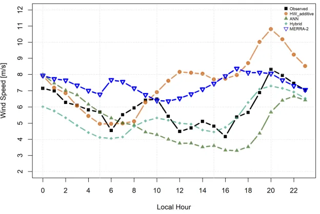
3.2.2. Based on 60 days of data
398
Figures 9 and 10 present the forecast for the day 31/11/2004 using 60 days of the temporal series
399
(01/10/2004 to 29/11/2004) for the measurements of the TA-01 and TA-02 towers, respectively.
400
For the TA-02 tower, the ANN model can be seen to follow the variability of the observed wind
401
speed data for up to 8 predicted hours. The model is unable to capture the small wind speed
402
variations that occur during the day, smoothing its results. The stochastic Holt-Winters model
403
overestimates after 11 predicted hours, but it follows the trends of the observations until 18
404
predicted hours, capturing the variability of wind. The hybrid model, therefore, showed a smoothed
405
pattern of the predicted wind speed with respect to the observations, and even so it underestimated
406
results most of the time. MERRA-2 overestimates results in relation to the observed data in the
407
temporal series, representing the behavior only in the first hours (until 6am) and last hours (after
408
21pm) predicted for the day 30/11/2004.
409
Table 6 shows the forecast skills of the models and the reanalysis with the observations. The
410
lowest values can be found in the hybrid model, whose RMSE and MAE were 0.91 m/s and 0.80 m/s.
411
The largest results were found in the Holt-Winters model (RMSE: 2.09 m/s and MAE: 1.68 m/s). The
412
correlation coefficient was also high in the hybrid model and low in the MERRA-2 reanalysis.
413
415
Figure 9. Comparison between the observed series, those predicted by the models and the MERRA-2 reanalysis
416
for the TA-01 tower on 31/11/2004.
417
Table 6. Residuals of the models and the reanalysis with the observations (TA-01) for 60 days of
418
forecasting, in m/s.
419
Holt-Winters ANN Hybrid MERRA-2
RMSE 2.09 1.39 0.91 1.75
MAE 1.68 1.19 0.80 1.41
r 0.47 0.66 0.80 0.23
420
For the TA-02 tower (Figure 10), one can see that the models follow the observed diurnal wind
421
speed data, but they underestimate and overestimate them at certain specific times. The ANN model
422
underestimates the first hours and overestimates the predicted wind speeds from 11:00am to
423
18:00pm. The Holt-Winters model underestimates most of the period and follows a behavior
424
consistent with the observed data between 8:00am and 20:00pm. The hybrid model approximates the
425
observed data most of the time, mainly between 5:00am and 8:00am.
426
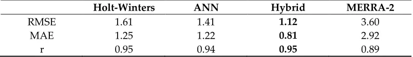
Table 7 shows the forecast skills of the models and the MERRA-2 reanalysis with the wind
427
speed observations. The lowest values can be found in the hybrid model, whose RMSE and MAE
428
were 1.12 m/s and 0.81 m/s. The highest values were found in the MERRA-2 reanalysis, with RMSE
429
and MAE values of 3.60 m/s and 2.92 m/s. The correlation coefficients were higher for all models in
430
this period.
431
444
Figure 10. Comparison between the observed series, those predicted by the models and the MERRA-2
445
reanalysis for the TA-02 tower on 31/11/2004.
446
Table 7. Residuals of the models and the reanalysis with the observations (TA-02) for 60 days of
447
forecasting, in m/s.
448
Holt-Winters ANN Hybrid MERRA-2
RMSE 1.61 1.41 1.12 3.60
MAE 1.25 1.22 0.81 2.92
r 0.95 0.94 0.95 0.89
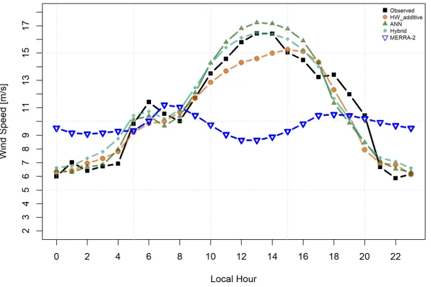
3.2.3. Based on 90 days of data
449
Figures 11 and 12 present the forecast for the day 31/12/2004 using 90 days of observations
450
(01/10/2004 to 29/12/2004) for the locations of the TA-01 and TA-02 towers, respectively.
451
For the TA-01 tower (Figure 11), the hybrid model underestimates the data observed in the
452
early hours and comes close to the observations between 11:00am and 14:00pm. The ANN model
453
overestimates the observations between the predicted hours of 7:00am and 20:00pm. The
454
Holt-Winters model underestimates the observed data until 15:00pm, coinciding with the original
455
series between 16:00pm and 19:00pm, after which it underestimates results again. The MERRA-2
456
reanalysis overestimates the original data in most of the time series.
457
Table 8 shows the residuals of the models and the reanalysis with the observed data. The lowest
458
errors can be found in the hybrid model and the largest in the MERRA-2 reanalysis. The
459
Holt-Winters model showed a large error in this assessment.
460
461
462
463
464
465
467
Figure 11. Comparison between the series observed by TA-01, those predicted by the models and the MERRA-2
468
reanalysis for the day 30/12/2004.
469
Table 7. Residuals of the models and the reanalysis with the observations (TA-01) for 90
470
days of data, in m/s.
471
Holt-Winters ANN Hybrid MERRA-2
RMSE 1.76 1.70 1.52 1.90
MAE 1.45 1.48 1.13 1.57
r 0.51 -0.31 0.27 0.13
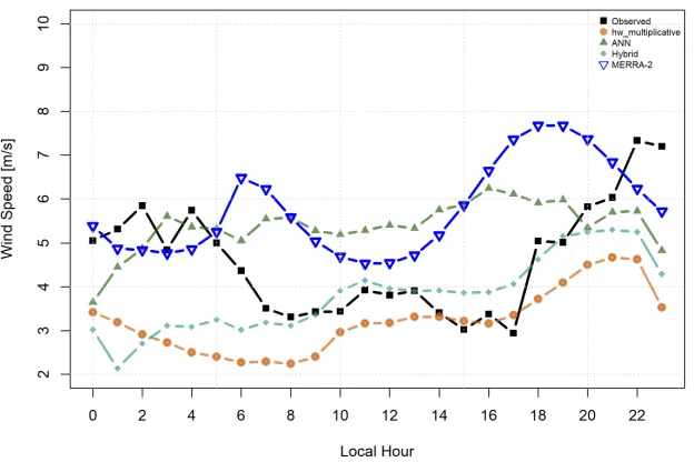
472
For the TA-02 tower, the Holt-Winters model overestimates the observed data at all times, but it
473
follows the behavior of the observations. Between the predicted hours of 23:00pm and 24:00pm, the
474
model coincides with the observed data. The hybrid and RNA models underestimate the observed
475
data during most of the time series and don't follow the behavior as well as the Holt-Winters model
476
(Figure 12).
477
Table 9 shows the residuals of the models and the reanalysis with the observations. The
478
smallest forecast skills are of the Holt-Winters model, with a RMSE and MAE of 2.14 and 1.62 m/s,
479
followed by the hybrid model with 2.27 and 1.84 m/s, respectively. The highest correlations are
480
482
Figure 12. Comparison between the observed series, those predicted by the models and the MERRA-2
483
reanalysis for the TA-02 tower on 30/12/2004.
484
Table 9. Residuals of the models and the reanalysis with the observations (TA-02) for 90 days of data,
485
in m/s.
486
Holt-Winters ANN Hybrid MERRA-2
RMSE 2.14 4.36 2.27 3.87
MAE 1.62 3.21 1.84 3.03
r 0.93 0.71 0.93 0.48
4. Discussion
487
4.1 Comparison with literature results
488
It is important to verify that these results of the errors in wind speed prediction this paper are in
489
agreement with the values found in similar literature studies. Reference [3] presented a study
490
involving the modeling of the monthly and hourly wind speed averages at a height of 10 meters in
491
the coastal Northeast region of Brazil for the prediction of wind speed for power generation with the
492
additive Holt-Winters model. According to the authors, when compared to the observed data, this
493
model showed a good fit with errors of RMSE and MAE of 0.50/0.57 m/s and 0.40/0.45 m/s for
494
monthly average wind speed forecasting, 1.38/1.55 m/s and 1.03/1.19 m/s for hourly average wind
495
speed forecasting, respectively. However, in studies like these applied to wind power generation,
496
the positioning of the measuring equipment must be installed at the top of the station (upper
497
anemometer) at a height from the ground equal to the axes of the wind park turbines and at least 50
498
meters from the ground, in accordance with the technical standards [32]. Reference [33] indicate the
499
measurement level of the primary wind speed measurement, which is mainly relevant for
500
determining the hub height wind conditions, shall be at least 2/3 of the planned hub height.
501
Currently the wind turbines in Brazil are being implanted at over 100 m height. Reference [10]
502
utilized the method of exponential smoothing, in particular the methods Holt-Winters additive and
503
multiplicative for 6 hours wind speed prediction at a height 50 m agl in the city São João Cariri
504
(Paraíba-Brazil) in order to apply the methodology. According author, the additive Holt-Winters
505
model presented better result than the multiplicative Holt-Winters model for 6 hours prediction in
506
the same series and data period of wind speed with errors of RMSE 2.0365 and 2.6197 m/s.
507
Reference [7] compare the performance of the ARIMA, ARIMAX and ANN models in an
509
attempt to forecast monthly wind speed averages at 3 locality’s in the coastal NEB (Fortaleza, Natal
510
and Paraíba). According to the authors, the ARIMAX model presented greater sensitivity to the
511
wind speed adjustment and prediction, the RMSE and MAE values found were
512
0.48(Fortaleza)/0.45(Natal)/0.71(Paraíba) m/s and 0.37(Fortaleza)/0.37(Natal)/0.54(Paraíba) m/s,
513
respectively. The authors proposed that, likely, with the increase in the number of training vectors
514
for the ANN model, its performance will improve and its statistical errors. Reference [6] proposed an
515
improved radial basis function neural network with an error feedback scheme to forecast short-term
516
wind speed and wind power, with parameter initialization method and the inclusion of the shape
517
parameter in the Gaussian basis function of each hidden neuron, used to search better initial center
518
and standard deviation values. Results show that the forecast accuracy by proposed model is better
519
compared to the other neural network-based models. Reference [34] used wind speed monthly
520
average data at 10 m agl of 28 meteorological stations operated by the Nigeria Meteorological
521
Services (NIMET) where were used as training (18 stations) and testing (10 stations) in the ANN
522
model. The ANN model consisted of 3-layered, feed-forward, back-propagation network with
523
different configurations. The proposed is used ANN model in the predicting of wind speed monthly
524
average. The results indicate high accuracy in the predicting of wind speed, with the correlation
525
coefficient between the predicted and the observed of 0.938, which shows the effectiveness of this
526
model.
527
In [17] developed a methodology for the short-term forecasting of wind power generation with
528
the modified ARIMAX model, which is based on the Box-Jenkins methodology, through which an
529
adjustment of models is obtained for the time series of observations so that the residuals are around
530
zero. The predicted and observed wind data as well as the actual wind power data were used as
531
inputs of the dynamic models. No satisfactory result was found among the models used, and this
532
has made the develop more research on wind forecasting geared to wind power generation [17].
533
In the study [22], the authors proposed a hybrid modeling method for the short-term wind
534
speed forecast for wind power generation, using data collected from an anemometric tower at a
535
height of 20 meters of (which also does not follow the standard) located in Beloit (Kansas/USA) in
536
the period from 2003 to 2004. The results showed that the hybrid modeling method for this variable
537
provides better predictions when compared to other methods, resulting in a MAE (m/s) ranging
538
from 0.016 to 0.52 in this study. In our study, the hybrid methodology also produced satisfactory
539
results. Reference [3] presented a combined hybrid model of the ARIMAX-ANN and
540
Holt-Winters-ANN models to predict the wind speed in terms of hourly means, being efficient in the
541
producing adjustments to the observed data of the studied regions. The authors showed the quality
542
of the proposed hybrid model is the low statistical analysis of errors values, for example, the RMSE
543
and MAE of 0.46/0.41 m/s and 0.35/0.32 m/s (locality: Fortaleza/Natal), especially when compared to
544
the ARIMAX, ANN and Holt-Winters models with errors values high for the RMSE e MAE. In [21]
545
proposed a hybrid short-term wind speed forecasting model at two cases studies. The results from
546
two cases show that the proposed hybrid model offers greater accuracy which relationship to the
547
other compared models (Persistent and ARIMA) in short-term wind speed forecasting. The hybrid
548
model ( showed the lowest values of error statistics, for
549
example, for the MAE it was possible to find values of 0.5132 m/s, versus that of 0.582 m/s and 0.5242
550
m/s, for the models of Persistent and ARIMA, respectively. Reference [14] proposed a hybrid
551
forecasting approach involving the statistics techniques EWT-CSA-LSSVM for short-term wind
552
speed prediction from a windmill farm located in northwestern China. The hybrid model showed
553
results suggest that the developed for wind speed forecasting method yields better predictions
554
compared with those of other models with the lower RMSE and MAE of 0.58 and 0.57 m/s errors.
555
556
557
558
5. Conclusions
560
561
Most research with wind data in Brazil is done through databases with little coverage,
562
especially with wind towers. Most of these studies are done by private companies and are not
563
publicly available for research. On the other hand, the monitoring via meteorological stations
564
features a series of errors. These facts contributed to make the development of this study difficult,
565
since there are no long wind speed time series available observed at 50 meters in height.
566
Given the difficulty of obtaining good temporal series and likely good results in the studies, this
567
article eventually became a mechanism for discovery and the exploration of alternative methods. As
568
for the modeling of the diurnal wind variability, the MERRA-2 reanalysis, which is the most recent
569
version, did not capture this variability well. The Holt-Winters model, which models the seasonality
570
and trend components, showed a good fit, but time series of several years are needed to better
571
capture these parameters and thus provide more satisfactory results. Finally, the best fits for the
572
forecast were found using the hybrid methodology. This method can be applied for the planning of
573
operations, maintenance and deployment of wind turbines, since accurate predictions minimize
574
technical and financial risks.
575
6. Patents
576
Author Contributions: This article has three authors. Paulo Sérgio Lucio conceived of the research idea and
577
gave suggestions. Moniki Dara de Melo Ferreira carried out the research, analyzed the data, developed the
578
scripts and drafted the article. Alexandre Torres Silva dos Santos has contributed with the research of articles,
579
the simulations, tips and revisions.
580
Acknowledgments: The Postgraduate Program of Climate and Atmospheric Sciences at Federal University of
581
Rio Grande do Norte and the Laboratory of Maps and Energetic Resources Data at Center for Technologies of
582
Gas and Renewable Energies supported this article.
583
Conflicts of Interest: The authors declare no conflict of interest.
584
Appendix A
585
Algorithm to Calculate wind speed forecasting short-term using Holt-Winters, ANN and
586
Hybrid models.
587
588
R-Code:
589
590
# Algorithm to calculate using Holt-Winters, ANN and Hybrid models
591
# Authors: Moniki Melo (UFRN) and Alexandre Santos (CTGAS-ER)
592
593
# Load add-on packages
594
595
library(stats)
596
library(tseries)
597
library(forecast,warn.conflicts=TRUE)
598
library(forecastHybrid)
599
600
# Data wind speed of BELO JARDIM - TA01
601
# Open file wind speed observational data
602
603
data_TA01 <- read.csv("belojardim_data.csv",header=T,sep=";",dec=",")
604
# Set the column of a matriz object
606
607
colnames(data_TA01)<-c("date","Wind_speed")
608
609
# The database is attached to the R search path (data wind speed of the TA01)
610
# This means that the database is searched by R when evaluating a variable, so objects in the datab
611
ase can be accessed by simply giving their names.
612
attach(data_TA01)
613
# Return the First or Last Part of an Object
614
615
head(data_TA01)
616
## date Wind_speed
617
## 1 01/10/2004 00:00 6.182
618
## 2 01/10/2004 01:00 6.517
619
## 3 01/10/2004 02:00 5.845
620
## 4 01/10/2004 03:00 5.125
621
## 5 01/10/2004 04:00 5.137
622
## 6 01/10/2004 05:00 3.798
623
# Holt-Winters-additive model
624
625
# 30 days - file based in this period of wind speed observed
626
627
data30days=data.frame(Wind_speed[1:720])
628
629
# Creating an time series with frequency of 24-hours
630
631
belojardim.ts=ts(data30days,freq=24)
632
633
# The Holt-Winters-additive filtering of wind speed time series.
634
# Unknown parameters are determined by minimizing the squared prediction error.
635
# Default configuration
636
637
belojardim.hw <- HoltWinters(belojardim.ts,seasonal="additive")
638
639
# Result of the Holt-Winters-additive
640
641
## $names
643
## [1] "fitted" "x" "alpha" "beta"
644
## [5] "gamma" "coefficients" "seasonal" "SSE"
645
## [9] "call"
646
##
647
## $class
648
## [1] "HoltWinters"
649
# stats package documentation – Holt-Winters Filtering
650
# Description
651
652
# An object of class "HoltWinters", a list with components:
653
654
# fitted : A multiple time series with one column for the filtered series
655
# as well as for the level, trend and seasonal components, estimated
656
# contemporaneously (that is at time t and not at the end of the series).
657
# x : The original series
658
# alpha : alpha used for filtering
659
# beta : beta used for filtering
660
# gamma :gamma used for filtering
661
# coefficients: A vector with named components a, b, s1, ..., sp containing the
662
# estimated values for the level, trend and seasonal components.
663
# seasonal: The specified seasonal parameter
664
# SSE : The final sum of squared errors achieved in optimizing
665
# call : The call used
666
667
# Result of the parameters: Holt-Winters-additive model
668
669
belojardim.hw$seasonal
670
## [1] "additive"
671
belojardim.hw$beta
672
## [1] 0
673
belojardim.hw$gamma
674
## [1] 0.9505823
675
belojardim.hw$SSE
676
## [1] 581.0709
677
678
# Forecast for the next 24-hours: forescat() function
679
forecast_24horas_hw <- forecast(belojardim.hw,h=24)
681
682
# Artificial Neural Networks model
683
# nnetar() function
684
# Default configuration
685
# Neural Network Time Series Forecasts
686
687
belojardim_ann <- nnetar(belojardim.ts)
688
689
# values of the arguments: parameters of model
690
691
attributes(belojardim_ann)
692
## $names
693
## [1] "x" "m" "p" "P" "scalex"
694
## [6] "size" "subset" "model" "nnetargs" "fitted"
695
## [11] "residuals" "lags" "series" "method" "call"
696
##
697
## $class
698
## [1] "nnetar"
699
# forecast package documentation – Neural Network Time Series Forecasts
700
# Description
701
# P - Number of seasonal lags used as inputs.
702
# p - Embedding dimension for non-seasonal time series. Number of non-seasonal lags used as input
703
s. For non-seasonal time series, the default is the optimal number of lags (according to the AIC) for
704
a linear AR(p) model. For seasonal time series, the same method is used but applied to seasonally a
705
djusted data (from an stl decomposition).
706
# size - Number of nodes in the hidden layer. Default is half of the number of input nodes (includi
707
ng external regressors, if given) plus 1.
708
# model - Output from a previous call to nnetar. If model is passed, this same model is fitted to y
709
without re-estimating any parameters.
710
belojardim_ann$m
711
## [1] 24
712
belojardim_ann$P
713
## [1] 1
714
belojardim_ann$p
715
belojardim_ann$size
717
## [1] 14
718
belojardim_ann$model
719
## Average of 20 networks, each of which is
720
## a 27-14-1 network with 407 weights
721
## options were - linear output units
722
forecast_24horas_ann <- forecast(belojardim_ann,h=24)
723
724
# Hybrid Model
725
# Default configuration
726
727
belojardim_hybrid <- hybridModel(belojardim.ts,models="nst")
728
## Fitting the nnetar model
729
## Fitting the stlm model
730
## Fitting the tbats model
731
# Forecast for the next 24-hours: forescat() function
732
# Default configuration
733
734
forecast_24horas_ann <- forecast(belojardim_hybrid,h=24)
735
# End of code
736
737
Appendix B
738
Algorithm to calculate the errors of the predictions by indices RMSE and MAE and Person
739
Correlation and plot of the graphics.
740
741
R-Code:
742
# Function : Calculate error
743
# Function to calculate Root Mean Squared Error (RMSE)
744
RMSE <- function(result) {
745
sqrt(mean(result^2))
746
}
747
# Function to calculate Mean Absolute Error (MAE)
748
MAE <- function(result) {
749
}
751
# Calculate error
752
# result <- predicted - observed
753
# Error of the Holt-Winters model
754
result <- forecast_24horas_hw$mean - data_TA01$Wind_speed[721:744]
755
round(RMSE(result),2)
756
round(MAE(result),2)
757
# Calculate Pearson correlation coefficient
758
759
round(cor(forecast_24horas_hw$mean,data_TA01$Wind_speed[721:744]),2)
760
# Plot graphics and saving in format tiff (vector)
761
# Defining time for cycle 24 hours
762
763
time <- c("00:00", "01:00", "02:00", "03:00", "04:00", "05:00", "06:00", "07:00",
764
"08:00", "09:00", "10:00","11:00","12:00","13:00","14:00","15:00",
765
"16:00","17:00","18:00","19:00","20:00","21:00","22:00","23:00")
766
hour.time <- strptime(time,"%H:%M")
767
768
# Open file wind speed observational data and predicted by models
769
770
dados <- read.csv("valores-belojardim24_30dias.csv",head=T,sep="",dec=",")
771
attach(dados)
772
head(dados)
773
## data hora obs hw_aditivo hw_mult rna hybrid merra2
774
## 1 2004-10-31 00:00 6.828 6.011 6.7630 6.151 6.440 6.729
775
## 2 2004-10-31 01:00 6.825 4.610 5.5218 6.100 5.809 6.761
776
## 3 2004-10-31 02:00 5.685 4.169 5.0910 5.998 5.447 6.626
777
## 4 2004-10-31 03:00 6.260 3.674 4.7000 6.225 5.138 6.789
778
## 5 2004-10-31 04:00 5.730 3.279 4.4010 6.057 4.701 6.961
779
## 6 2004-10-31 05:00 4.680 3.574 4.5070 5.845 4.707 7.071
780
# Saving file in vector (tiff)
781
782
tiff("belojardim_paper_30days.tiff", width = 8, height = 6, units = 'in', res = 300,compression =
783
'lzw')
784
785
xlab="Local Hour",ylab="Wind Speed [m/s]")
787
lines(0:23,hw_aditivo,col=rgb(0.8,0.4,0.1,0.7) , lwd=3 , pch=19 , type="b" )
788
lines(0:23,rna,col=rgb(0.2,0.4,0.1,0.7), lwd=3 , pch=17 , type="b" )
789
lines(0:23,hybrid,col=rgb(0.225,0.64,0.5,0.7), lwd=3 , pch=18 , type="b" )
790
lines(0:23,merra2,col="blue", lwd=3 , pch=25 , type="b" )
791
792
axis(side=1, at=seq(0,23,by=2))
793
axis(side=2, at=seq(1, 10, by=1))
794
box()
795
grid()
796
797
# Legend of the graphics
798
799
legend("topright",
800
legend = c("Observed", "hw_additive","ANN","Hybrid","MERRA-2"),
801
col = c("black",rgb(0.8,0.4,0.1,0.7),
802
rgb(0.2,0.4,0.1,0.7),rgb(0.225,0.64,0.5,0.7),"blue"),
803
pch = c(15,19,17,18,25),
804
bty = "n",
805
pt.cex = 1,
806
cex = 0.6,
807
text.col = "black",
808
horiz = F,)
809
810
# End of the code
811
812
dev.off()
813
Appendix C
814
Tables: Main characteristics of ANNs and hybrid (nnetar-stlm-tbats functions) models produced
815
in R software.
816
817
Belo Jardim - Hour Based on 30 days of data
p P Size(k) m Weights Average of Network
26 1 14 24 393 20
Based on 60 days of data
p P Size(K) m Weights Average of Network
25 1 13 24 352 20
Based on 90 days of data
p P Size(K) m Weights Average of Network
25 1 13 24 352 20