Power and Timing Side Channels for PUFs and
their Efficient Exploitation
Ulrich R¨uhrmair, Xiaolin Xu, Jan S¨olter, Ahmed Mahmoud, Farinaz Koushanfar, Wayne Burleson
Abstract—We discuss the first power and timing side channels on Strong Physical Unclonable Functions (Strong PUFs) in the literature, and describe their efficient exploitation via adapted machine learning (ML) techniques. Our method is illustrated by the example of the two currently most secure (CCS 2010, IEEE T-IFS 2013) electrical Strong PUFs, so-called XOR Arbiter PUFs and Lightweight PUFs. It allows us for the first time to tackle these two architectures with a polynomial attack complexity.
In greater detail, our power and timing side channels provide information on the single outputs of the many parallel Arbiter PUFs inside an XOR Arbiter PUF or Lightweight PUF. They indicate how many of these single outputs (in sum) were equal to one (and how many were equal to zero) before the outputs entered the final XOR gate. Taken for itself, this side channel information is of little value, since it does not tell which of the single outputs were zero or one, respectively. But we show that if combined with suitably adapted machine learning techniques, it allows very efficient attacks on the two above PUFs, i.e., attacks that merely use linearly many challenge-response pairs and low-degree polynomial computation times. Without countermeasures, the two PUFs can hence no longer be called secure, regardless of their sizes. For comparison, the best-performing pure modeling attacks on the above two PUFs are known to have an exponential complexity (CCS 2010, IEEE T-IFS 2013).
The practical viability of new our attacks is firstly demon-strated by ML experiments on numerically simulated CRPs. We thereby confirm attacks on the two above PUFs for up to 16 XORs and challenge bitlengths of up to 512. Secondly, we execute a full experimental proof-of-concept for our timing side channel, successfully attacking FPGA-implementations of the two above PUF types for 8, 12, and 16 XORs, and bitlengths 64, 128, 256 and 512. In earlier works (CCS 2010, IEEE T-IFS 2013), 8 XOR architectures with bitlength 512 had been explicitly suggested as secure and beyond the reach of foreseeable attacks.
Besides the abovementioned new power and timing side channels, two other central innovations of our paper are our tailormade, polynomial ML-algorithm that integrates the side channel information, and the implementation of Arbiter PUF variants with up to 16 XORs and bitlength 512 in silicon. To our knowledge, such sizes have never been implemented before in the literature. Finally, we discuss efficient countermeasures against our power and timing side channels. They could and should be used to secure future Arbiter PUF generations against the latter.
Keywords-Physical unclonable functions (PUFs), side channel attacks, power side channel, timing side channel, modeling attacks, machine learning, hardware security
Ulrich R¨uhrmair, [email protected]
Xiaolin Xu and Wayne Burleson are with the University of Massachusetts Amherst, Amherst, MA 01003, USA.
Jan S¨olter is with the Freie Universit¨at Berlin, 14195 Berlin, Germany. Ahmed Mahmoud is with the Technische Universit¨at M¨unchen, 80333 M¨unchen, Germany.
Farinaz Koushanfar is with Rice University, Houston, TX 77005, USA.
I. INTRODUCTION
Most modern cryptographic and security schemes are built on the concept of a secret key. This forces current hardware to contain a piece of digital information that is, and remains, unknown to the adversary. This requirement can be difficult to uphold in practice: Physical attacks like invasive, semi-invasive or side-channel attacks, as well as software attacks like malware, can lead to key exposure and full security breaks. Indeed, one of the main motivations in the development of Physical Unclonable Functions (PUFs) was their promise to better protect secret digital keys in vulnerable hardware systems. A PUF is an (at least partly) disordered physical system P that can be excited with external stimuli or so-called challenges Ci. It reacts with corresponding responses
Ri, which depend on the challenge and on the micro- or
nanoscale structural disorder that is present in the PUF. It is assumed that this disorder cannot be cloned or reproduced exactly, not even by the PUF’s original manufacturer, and that it is unique to each PUF. Assuming efficient error correction on the noisy PUF responses, each PUF P thus implements a unique and individual functionfP that maps challengesCi
from an admissible challenge set to responsesRi =fP(Ci).
The tuples(Ci, Ri)are thereby usually called the
challenge-response pairs (CRPs) of the PUF.
Due to their complex internal structure, PUFs promise to avoid some of the shortcomings of classical digital keys. It is usually harder to read out, predict, or derive PUF-responses than to obtain digital keys that are stored in non-volatile memory. The PUF-responses are only generated when needed, which means that no secret keys are present permanently in an easily accessible digital form. Furthermore, certain types of PUFs promise some natural tamper sensitivity, as their exact behavior depends on minuscule manufacturing irregularities in different layers of the IC. Removing or penetrating these layers is often assumed to automatically change the PUF’s read-out values.
keys and standard computational assumptions (such as the hardness of factoring) are involved. Overall, the assumed secu-rity advantages of PUFs have attracted considerable attention within the security community over the last decade.
a) Recent Attacks on PUFs and Related Work: In the last years, an increasing number of attacks on PUFs have been published. Some of them were specifically developed for this new primitive, while others are an adaption of known strategies to the PUF case. Not all attacks apply to every PUF design in the same manner. In order to categorize existing work, it makes sense to distinguish between the two major PUF types of “Weak PUFs”and“Strong PUFs”1 .
Let us start with Strong PUFs. The currently most relevant attack form on this PUF type are machine-learning (ML) based modeling attacks, which have been pursued by a large number of authors [13], [22], [17], [16], [10], [3], [32], [34]. They are particularly well applicable to Strong PUFs, since this PUF type has a publicly accessible CRP interface, which allows the collection of the large numbers of CRPs that are required in these attacks. Two recent works from CCS 2010 and IEEE T-IFS 2013 [32], [34], which represent the current state of the art, have indeed succesfully tackled a considerable number of Strong PUF designs, including standard Arbiter PUFs, XOR Arbiter PUFs, Feed-Forward Arbiter PUFs, Lightweight PUFs, and certain forms of Ring Oscillator PUFs [35], [32], [16]. The architectures with the highest ML-resilience were found to be XOR Arbiter PUFs [35], [32] and Lightweight PUFs [16]. They could only be be attacked efficiently if they are composed of at most five or six single parallel Arbiter PUFs with bitlength 64 or 128 each [32], [34]. To give a full picture to the readers, some concrete results of [32], [34] are summarized in Table I. They show that the CRP consumption and training times grow substantially for larger number of XORs k and bitlengths n. The authors of [32] estimate that the growth is exponential in the number of XORs k, and polynomial to the degree k in the bitlength n. Furthermore, from all PUFs examined in [32], [34], the XOR Arbiter PUF and the Lightweight PUF possess the highest ML resilience, with the latter yet being somewhat harder to break.
To summarize, no efficient attacks on Lightweight PUFs and XOR Arbiter PUFs with bitlengths of 256 or more and with 6 XORs or more were possible prior to this work, and also no polynomial time ML algorithms for attacking these structures were known. Note here that the instability of XOR Arbiter PUFs and Lightweight PUFs with k XORs grows exponentially in k. This puts a natural limit on the number of XORs that can be used. The authors of [32], [34] hence explicitly suggested the use of XOR Arbiter PUFs and Lightweight PUFs with eight parallel Arbiter PUFs (with “8 XORs”) and bitlengths 512 as both stable and secure against existing modeling attacks.
Another attack on Strong PUFs that is relevant in our con-text has been presented recently by Delvaux and Verbauwhede [3]. They combine a noise-based side channel with analyti-cal modeling techniques in order to attack standard Arbiter
1For an explanation of Weak and Strong PUFs and other PUF types, we refer the reader to R¨uhrmair et al. [32], [34], [30].
PUFs (i.e., without any XORs). Interestingly, their modeling approach does not employ any machine learning algorithms. Their method is very attractive, but in its current form achieves slightly worse accuracy than ML-based modelingwithoutside channels (97% in [3] vs. 99% in [34]). It also has a higher CRP-consumption than pure ML-based modeling without side channels. This is in opposition to the attacks presented in this paper, actually drastically increase the performance of pure ML-based Strong PUF attacks.
Other recent attacks have mostly focused on so-calledWeak PUFs. Merli et al. attack the error-correcting module of Weak PUFs at TRUST 2011 [19], and EM analyses on ring oscillator PUFs (RO PUFs) have been carried out by the same group at WESS 2011 [20]. Nedospasov et al. describe successful invasive methods on SRAM PUFs at FDTC 2013 [21]. Finally, Helfmeier et al. report cloning attacks on SRAM PUFs at HOST 2013 [9].
Comparable cloning or invasive attacks on Strong PUFs have not been reported to this date. There is a reason for this: Typical Strong PUFs possess very many possible challenges and a complex response generation process, in which a large number of components interact to produce one single response. Successful physical cloning would require the accurate dupli-cation of all of these components in order to get all CRPs right. In the case of an Arbiter PUF, for example, it would involve successful tuning of all delay values in the subcomponents; or in the case of optical PUFs, it would require precise positioning ofallthe scattering centers in the PUF. This seems significantly harder than tuning the single output of typical Weak PUFs, for example tuning the start-up value of a single SRAM cell. Furthermore, an invasive read-out of the single response of a Weak PUF is obviously simpler than reading out the exponentially many CRPs of typical Strong PUFs.
Finally, a number of protocol attacks on advanced Strong PUF schemes such as key exchange or oblivious transfer have been presented recently at CHES 2012, IEEE S&P 2013, and other venues [31], [27], [28], [29]. They describe relevant methods, but lie beyond the topic of this paper, which focuses on hardware attacks.
b) Our Contributions: This work combines for the first time machine learning based modeling with side channel information to reach new performance levels in Strong PUF attacks. We illustrate our methods by the example of XOR Arbiter PUFs and Lightweight PUFs, which are the two most secure and practical electrical Strong PUFs according to the current state of the art [32], [34]. We show that our new approach allows the first successfully attacks on these two designs for up to 16 internal, parallel single Arbiter PUFs (i.e., for “16 XORs”), and for bitlengths of up to 512. It also reduces, for the very first time, the CRP consumption of the attacks to linear, and the corresponding ML training times to low degree polyonmial.
PUF-Type No. of Bit Source of CRPs Prediction Training
XORs Length CRPs (×103) Rate Time
Arbiter PUF — 64 Simulation 2.5 99% 0.13 sec
128 5.5 0.51 sec
XOR Arb PUF
4 64 Simulation 12 99% 3:42 min
128 24 2:52 hrs
5 12864 Simulation 50080 99% 16:36 hrs2:08 hrs
6 12864 Simulation 200— 99% 31:01 hrs—
Lightweight PUF
4 64 Simulation 12 99% 1:28 hrs
128 500 59:42 min
5 64 Simulation 300 99% 13:06 hrs
128 1000 267 days
6 64 Simulation — 99% —
128 — —
TABLE I
STATE OF THEART OF MODELING ATTACKS ONARBITERPUFS, XOR ARBITERPUFS,ANDLIGHTWEIGHTPUFS,TAKEN FROM[32], [34]. ALL SHOWN RESULTS WERE OBTAINED ON SIMULATEDCRPS GENERATED BY THE ADDITIVE LINEAR DELAY MODEL[13], [32], [34]. THE TRAINING TIMES ARE
CALCULATED AS IF THEMLEXPERIMENT WAS RUN ON ONLYone singleCORE OFone singlePROCESSOR. USE OFkCORES WILL APPROXIMATELY REDUCE THEM BY1/k.
by the linear additive delay model carry over with very little performance loss to silicon CRPs. Furthermore, the same works [32], [34] showed that the ML method employed in this paper (i.e., logistic regression) possess substantial error tolerance. Reasonable noise levels in the side channel will not alter its performance significantly.
In addition, we carry out a full proof of concept on FPGA implementations of XOR Arbiter PUFs and Lightweight PUFs. In this process, we utilize an efficient, yet simple error correction method for our side channel that keeps noise levels particularly low. Our approach allows us to attack the two above PUFs for eight single parallel Arbiter PUFs (i.e., for “8 XORs”), and for bitlengths 128, 256 and 512. These sizes had been explicitly suggested as secure in earlier works without implementing them [32], [34]. To our knowledge, our FPGA-implementations of XOR Arbiter PUFs and Lightweight PUFs with 8 XORs and up to 512 bits are the first with comparably large sizes and complexities. We implement these regimes for the first time, and subsequently attack them successfully by our new methods.
Our attacks in practice require physical access to the PUF, which is part of the established Strong PUF attack model [32], [34]. Compared to earlier work [32], [34], they involve the collection of a relatively mild amount of CRPs, and lead to very short computation times. In fact, we empirically estimate the required CRPs to be linear in the size of the PUF (i.e., in the number of XORs and the bitlength), and the computation times to be low degree polynomial. This is in stark contrast to the estimated exponential CRP requirements and computation times of earlier methods on the two above PUF types [32], [34].
Our two side channels are the first power and timing side channel on PUFs discussed in the literature. They are also the first general side channels on Strong PUFs that can increase attack performance (compare above). Both tell an attacker the cumulative number of zeros and the cumulative number of ones in the internal outputs of all the single, parallel Arbiter PUFs within an XOR Arbiter PUF or Lightweight
PUF structure. Our power side channel draws its information from closely monitoring the power consumption of the PUF, and from tracing the loads that arise when the final latches that act as “arbiters” in Arbiter PUF implementations switch to one or remain zero. Our timing side channel is based on marking different response patterns with corresponding timing signatures. With the extracted timing signature, we can reversely conclude the composition of multiple individual responses (before the XOR function), deriving the cumulative number of zeros and the cumulative number of ones.
Besides the above new side channels and the first silicon implementation of Arbiter PUF variants with 8 XORs and bitlength up to 512, a fourth central contribution of this paper is the development of a novel, tailormade non-linear regression algorithm. Our algorithm can efficiently exploit the above side channel information on the cumulative number of zeros and ones. To this end, a differentiable model of the side channel in-formation was developed. This new algorithm strongly reduces the complexity of the ML problem associated to XOR Arbiter PUFs and Lightweight PUFs: From the exponential complexity of earlier algorithms without side channel information [32], [34] to a linear CRP consumption and low-degree polynomial runtimes in this paper.
At the end of this work, we discuss countermeasures against our side channel attacks, which could and should be put in place in future Arbiter PUF generations. The differential output architecture that we suggest for thwarting power side channels even appears to have applications elsewhere, for example in detecting or correcting output errors in Arbiter PUFs. We also discuss several possibilities to encounter timing side channels, most importantly a method for the construction of an isochronous hardware.
XOR
b1 b2 b3 bn-1 bn
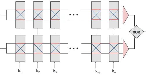
Fig. 1. An XOR Arbiter PUF composed of two single, parallel Arbiter PUFs, also referred to as “2-XOR Arbiter PUF” or “Arbiter PUF with two XORs”. The 1-bit outputs of the two single arbiters (red triangles) enter a final XOR gate to produce a 1-bit overall output. The shown structure has bitlengthn.
CRPs and side channel info. Section VII leads a full proof of concept for combined modeling and timing side channel attacks on FPGA implementations of XOR Arbiter PUFs and Lightweight PUFs. Section VIII describes countermeasures against our side channels. Section IX concludes the paper.
II. BACKGROUND ANDSOMEML METHODOLOGY
A. Arbiter PUF Variants
Arbiter PUFs and variants thereof were among the first electrical PUFs [6], [7], [12], [35], and are currently among the most widespread and best investigated PUF designs. The three variants relevant for this work are described below.
d) Arbiter PUFs: The basic, standard Arbiter PUF has been introduced and discussed in [7], [12], [35]. It consists of a sequence of n stages, for example multiplexers. Two electrical signals race simultaneously and in parallel through these stages. Their exact paths are determined by a sequence of nexternal bitsb1· · ·bn applied to the stages, whereby the
i-th bit is applied at the i-th stage. Ifbi = 0, then the paths
run “in parallel” through the multiplexers, and if bi= 1, they
cross each other and change position. After the last stage, an “arbiter element” consisting of a latch determines whether the upper or lower signal arrived first and correspondingly outputs a zero or a one. The external bits are usually regarded as the challengeC of this PUF, i.e.,C=b1· · ·bn, and the output of
the arbiter element is interpreted as their response R. See [7], [12], [35] for further details. The parameternis often referred to as the bitlength of the Arbiter PUF.
e) XOR Arbiter PUFs: One possibility to strengthen the resilience of arbiter architectures against machine learning attacks, which has been suggested in [13], [35], is to employ kindividual Arbiter PUFs in parallel, each withnstages (i.e., each with bitlength n). The same challenge C is applied to all of them, and their individual outputs ri are XORed in
order to produce a global response oXOR. We denote such
an architecture as“k-XOR Arbiter PUF”or as“XOR Arbiter PUF with k XORs”. The case of a 2-XOR Arbiter PUF is illustrated in Figure 1.
f) Lightweight PUFs: Another type of delay-based PUF, which is often termed Lightweight Secure PUF or Lightweight
PUF for short, has been introduced in [16]. It is similar to the XOR Arb-PUF of the last paragraph. At its heart are k individual standard Arb-PUFs arranged in parallel, each with n stages (i.e., with bitlength n), which produce k individual outputs r1, . . . , rk. These individual outputs are XORed to
produce a multi-bit response o1, ..., om of the Lightweight
PUF, according to the formula
oj=
⊕
i=1,...,x
r(j+s+i)modk for j= 1, . . . , m. (1)
Thereby the values for m (the number of output bits of the Lightweight PUF),x(the number of valuesrj that influence
each single output bit) ands(the circular shift in choosing the xvaluesrj) are variable design parameters.
Another difference to the XOR Arbiter PUFs lies in thek inputs C1 = b11· · ·b1n, C2 = b21· · ·b2n, . . . , Cl = bl1· · ·bln
which are applied to thek individual Arbiter PUFs. Contrary to XOR Arbiter PUFs, it does not hold thatC1=C2=. . .= Ck =C, but a more complicated input mapping that derives
the individual inputs Ci from the global input C is applied.
This input mapping constitutes the most significant difference between the Lightweight PUF and the XOR Arbiter PUF. We refer the reader to [16] for further details.
From the many possible variants of Lightweight PUFs that are enabled by the above parameters m, x and s, we concentrate on the following version in this paper: We consider Lightweight PUFs composed of k parallel standard Arbiter PUFs, and apply the standard input mapping described in [16]. For the output, we take the XOR of all responses of the k parallel Arbiter PUFs. In terms of the bitwise security of the output, this is the most secure variant of the Lightweight PUF: XORing less than k single responses for one response leads to a worsened bit security of the output. For these reasons, exactly the same variant of the Lightweight PUF has been considered in earlier works on the topic [32], [34]. Sticking with this variant furthermore ensures comparability of our data and earlier results [32], [34].
B. Logistic Regression with RProp
From earlier work [32], [34], it is known that an adapted form of logistic regression (LR) performs best on the three PUFs of the last Section II-A. LR is a well-investigated super-vised machine learning framework, which has been described, for example, in [1]. In its application to PUFs with single-bit outputs, each challengeC=b1· · ·bkis assigned a probability
p(C, r|w⃗)that it generates a outputr ∈ {0,1} ). The vector ⃗
w encodes the relevant internal parameters, for example the particular runtime delays, of the individual PUF. The proba-bility is given by the logistic sigmoid σ(x) = (1 +e−x)−1 acting on a functionf(w, C⃗ )parametrized by the vectorw⃗ as
p(C, r|w⃗) =rσ(f) + (1−r)(1−σ(f)). (2)
likelihood of observing this set is maximal, respectively the negative log-likelihood is minimal:
ˆ ⃗
w=argminw⃗ l(M, ⃗w) =argminw⃗ ∑
(C, r)∈ M
−ln p(C, r|w⃗)
(3) As there is no analytical solution to determine the optimal parameter vector w⃗ˆ, it has to be optimized iteratively, e.g., using the gradient information
∇l(M, ⃗w) = ∑
(C, r)∈ M
(σ(f(w⃗))−r)∇f(w⃗) (4)
From the different possible optimization methods, RProp [1] [25] has been identified as optimal in earlier ML works on PUFs [32], [34]. RProp makes a very big difference in convergence speed and stability of the LR algorithms (k-XOR Arbiter PUFs for medium or largekwere only learnable with RProp).
In general, logistic regression has the asset that the exam-ined problems need not be (approximately) linearly separable in feature space, as is required for successful application of support vector machines, for example, but merely differen-tiable.
C. Linear Additive Delay Model
It has become standard to describe the functionality of Arbiter PUF variants via an additive linear delay model [13], [32], [34]. The overall delays of the two racing signals are modeled as the sum of the delays in the stages. The final delay difference ∆ between the upper and the lower path in an n-bit Arbiter PUF is expressed as
∆ =w⃗T⃗Φ, (5)
wherew⃗ andΦ⃗ are vectors of dimensionn+ 1. The parameter vector w⃗ encodes the delays for the subcomponents in the Arbiter PUF stages, whereas the feature vector ⃗Φis solely a function of the applied n-bit challengeC [13], [32], [34].
In greater detail, the following holds. We denote by δ0i/1 the runtime delay in stage i for the crossed(1) respectively uncrossed(0) signal path. Then
⃗
w= (w1, w2, . . . , wk, wn+1)T, (6)
where w1 = δ10−δ11 2 , wi =
δi0−1+δi1−1+δ0i −δ1i
2 for all
i= 2, . . . , n, andwn+1= δ0n+δ 1 n
2 . Furthermore, ⃗
Φ(C⃗) = (Φ1(C⃗), . . . ,Φk(C⃗),1)T, (7)
whereΦl(C⃗) =∏n
i=l(1−2bi)for l= 1, . . . , n.
The output r of an Arb-PUF is determined by the sign of the final delay difference ∆:
r= Θ(∆) = Θ(w⃗T⃗Φ). (8)
with Θ being the Heaviside step function, i.e., Θ(x) = 0 if x < 0 andΘ(x) = 1ifx ≥ 0. Eqn. 8 shows that the vector w⃗ viaw⃗TΦ = 0⃗ determines a separating hyperplane in the space of all feature vectorsΦ⃗. Any challengesC that have their feature vector located on the one side of that plane give
response r = 0, those with feature vectors on the other side r= 1. Determination of this hyperplane allows prediction of the PUF and can be achieved by setting the decision function f in Eqn. 2 to the linear delay model f =w⃗T⃗Φ.
More complex architectures that use k standard Arbiter PUFs in parallel, possibly together with special input or output mappings, can then simply be modelled by using the linear additive delay model for each of the parallel Arbiter PUFs. Overall, this involves k feature vectors Φ⃗1, . . . , ⃗Φk derived
from the effective challenges at the individual Arbiter PUFs (given by the input mapping) andkweight vectorsw⃗1, . . . , ⃗wk:
o= Θ(
k
∏
i=1
∆i) = Θ( k
∏
i=1 ⃗
wiTΦ⃗i) (9)
Eqn. 9 defines a decision boundary at∏ki=1w⃗T
iΦ⃗i = 0. Any
challenges C that have their feature vector set ⃗Φ1, . . . , ⃗Φk
located on the one side of the boundary (e.g.o <0respectively an odd number of individual delays∆ismaller than zero) give
response r = 0, those with feature vectors on the other side r = 1. Determination of this boundary allows prediction of the PUF and can be achieved by setting the decision function f in Eqn. 2 to this boundaryf =∏ki=1w⃗T
i ⃗Φi. It implies an
optimization along the gradient in Eqn. 4:
∇f(w⃗j) =Φ⃗j
∏
i̸=j
⃗
wiTΦ⃗i (10)
This principle has been applied to the XOR Arbiter PUF and Lightweight PUF of this paper.
D. Numerical CRP Generation, Simulated Side Channels
A subset of the attacks presented in this paper are executed on simulated CRPs generated by the additive linear delay model of the last section. The simulated challenge-response pairs (CRPs) were generated in the following fashion: (i) The delay values for all single Arbiter PUFs within the respective PUF variant were chosen pseudo-randomly according to a standard normal distribution. We sometimes refer to this as choosing a certain PUF instance in the paper. In the language of Eqn. 5, it amounts to choosing the n+ 1 entries of the vector w⃗ pseudo-randomly according to a standard normal distribution. (ii) If a response of this PUF instance to a given challenge is needed, it is calculated by use of the delays selected in step (i). The delays of the two electrical signal paths are simply added up and compared. Or, again in the language of of Eqn. 5, the value of∆ is computed.
In a subset of our attacks, also simulated side channel information is used. The cumulative number of ones in the outputs of the single Arbiter PUFs was obtained directly from the above CRP simulation in the linear additive delay model, i.e., simply by adding up the outputs of the single, parallel Arbiter PUFs in the above CRP simulation. An analog statement holds for the cumulative number of zeros.
E. Training Set, Test Set, and Prediction Error
Fig. 2. The power tracking side channel analysis for a latch that had a transition to 1, with different driving loads, in SPICE simulation. The inset is the amount of drawn charges, which is calculated from the area under each curve. The amount of charges is linearly proportional with the number of gates, noting that the amount of charges normally drawn for a floating load should be subtracted.
trained ML algorithm when evaluated on the test set. For all ML experiments throughout this paper, each test set consisted of 10,000 randomly chosen CRPs. The size of the employed training sets varies, and is given individually on each occasion. The prediction rate is 1−ϵ.
The termNCRP (or simply“CRPs”) denotes the number of
CRPs employed in an attack. In the case of logistic regression (LR), which is the only ML algorithm employed in this paper, this number is always equal to the size of the training set.
F. Employed Computational Resources and Training Times
We used an Intel Xeon X5650 processor at 2.67GHz with 48 GB of RAM in all of our ML experiments, representing a worth of a few thousand Euros. All computation times (= “training times”) are calculated for one core of one processor of this hardware.
III. POWERSIDECHANNELS ONARBITERPUF VARIANTS
The basic concept of our power side channel is to apply power tracing to determine the transition from zero to one of the latches (=arbiter elements) that are part of Arbiter PUF based architectures. The power tracing technique is based on measuring the amount of current drawn from the supply voltage during any latch transition to one.
In order to validate our approach, we implemented a SPICE simulation that uses only one latch with three different outputs loading (floating output, output connected to one gate, and output connected to four gates). Figure 2 illustrates our results, and shows the different amount of current drawn for the three different output loading. The reason for having different values for the different loading is that an additional amount of charges is required to charge the capacitance of each gate. Hence, the amount of drawn charges, which is the integration of
the current curve, is linearly proportional with the number of gates. Taking into consideration, the amount of charges normally drawn in case of a floating load should be subtracted. Consequently, for extreme cases when all latches’ output in the device are zeros or all are ones, this power tracing technique would allow the attacker to determine these cases very easily. By applying this idea to XOR Arbiter PUFs and Lightweight PUFs, which utilize more than one single Arbiter PUF in parallel, one could determine the cumulative number of ones (and zeros) stored in the latches (arbiters) within the PUF. Following our above discussion, the power consumption will tell us the cumulative number of zeros and ones that are stored in the latches (or, in other words, the cumulative number of zeros and ones that is output by the single Arbiter PUFs before the large, final XOR gate. Please note, however, that we cannot derive which of the single Arbiter PUFs in an XOR Arbiter PUF have output one and which have output zero. We only know the overall number of zeros and ones before the XOR. Taken by itself, the side channel thus appears relatively worthless. We will nevertheless show that this basic information can boost PUF attacks significantly if it is used in the right manner in Section V.
IV. TIMINGSIDECHANNELS ONARBITERPUF VARIANTS
A. Delay Measurement Circuitry
Let us now describe our timing side channel approach, starting with our delay measurement circuit. It operates on the basis of FPGA reconfigurability. Figure 3 demonstrates an abstraction of the delay measurement concept and circuitry. To measure the timing of the circuit under test (CUT), three on-chip flip flops (FFs) connected to the on-chip clock are utilized:
Circuit-
under-test
FF
D
Launch
Flip Flop
Flip Flops
Sample
Flip Flops
Capture
D
FF
FF
D
V
DDBinary Challenge
T
Timing
Challenge
S D QE L
Fig. 3. The timing signature extraction circuit.
The clock signal with a period of2T is applied to the CUT when all the FFs are set to an initial value. For the sake of explanation, assume that the initial value of each FF is zero
and the CUT’s output, after applying the input, is expected to change from zero to one. At the clock’s rising edge, the launch FF sends a low-to-high signal to the CUT. At timeT, i.e., half the clock period, the sample FF samples the output at the falling clock edge. (Note the inverted clock signal at the sample FF.)
There are three possible scenarios for the value of the sample FF: (i) the CUT delay is less than T, in which case the sample FF will be set to the correct value (one); (iii) the CUT delay is (almost) equal to T and therefore the FF shall be in a transition mode; and (ii) the CUT delay is greater than T and thus the sample FF will not be set to the final value. As shown on the Figure, an XOR gate compares the values of the actual output and the sample FF. The capture FF would hold the comparison results for one clock cycle. In case (i), the comparison would demonstrate equal values of the two XOR inputs, while in case (iii) the two XOR inputs would differ, generating an error signal (one) at the capture FF. Case (ii) is trickier to predict, as the output signal in transition may be interpreted as zero or one at the input of the XOR gate with a certain probability.
We now perform a more careful timing analysis. Let tcut,
tc2Q, tskew, tsetS, tholdS, tsetC, tholdC, and txor denote the
values for the CUT, clock-to-Q of the launch FF, clock skew between the launch and sample FFs, the sample FF’s setup, the sample FF’s hold, the capture FF’s setup, the capture FF’s hold, and XOR timings respectively. If tp denotes the total
propagation delay from the moment the launch FF is clocked to the moment the signal passes through CUTs and settles at the sample FF, then tp=tcut+tc2Q−tskew.
In case of near equality oftpandT, i.e., scenario (ii) above,
because of the setup and hold timing violations the sample FF would enter a metastable point. The probability of the metastable point resolving to a zero or one value at the capture FF is a function of the proximity oftpandT. As an example,
in case of having equal T and tcut both clock and signal
simultaneously arrive at the sample FF. Thus, the metastable point resolves to a zeroor onewith equal probability.
When the XOR output at the capture FF does not demon-strate a discrepancy, the following relationship holds:
tholdC < tp< T −tsetS (11)
Astp enters the following interval,
T−tsetS< tp< T +tholdS (12)
the capture FF shows the output metastability.
Note that the probability of occurrence of timing errors demonstrates a periodic rise and fall pattern. First, the proba-bility of timing error rises astpgets closer to the upper bound
of Inequality above. The timing error would occur every cycle (with a high probability) once the following condition holds:
T+tholdS < tp<2T−(tsetC+txor) (13)
Next, once the value oftp exceeds the2T−(tsetC +tXOR)
in Equation 13, the timing error’s rate starts to decline. The fall in error probability is not because of the correctness of functionality, but it is because of the limitations of the capture FF in observing and recording the timing errors.
Equation 14 (below) demonstrates the transition from the scenario where there is a high probability of error in each clock cycle (Equation 13) to the scenario where no errors shall be detected (Equation 15).
2T−(tsetC+txor)< tp <2T+ (tholdC−txor) (14)
2T+ (tholdC−txor)< tp<3T−tsetS (15)
In case tp is larger than 3T −tsetS, the timing errors shall
not be hidden anymore. Indeed, the timing errors emerge and could be captured iftp is within the interval below:
3T−tsetS < tp<3T+tholdS (16)
Assuming that Inequality 17 holds, the timing errors would be detectable in each clock cycle:
3T+tholdS < tp<4T −(tsetC+txor) (17)
This rise and fall pattern repeats for integer multiplies of T; the maximum FPGA clock frequency sets an upper bound on this behavior. If the value of T >> txor andT >> tset and
T >> thold (for the FFs), it is possible to approximate the
intervals as n×T < tp <(n+ 1)×T where timing errors
shall be detected for oddnvalues.
Note that in Figure 3, the propagation delay of the CUT circuit may be different, in practice, for the low-to-high and high-to-low transitions. Suppose that one of them is greater than the other, e.g.,tlp→h< tpl→h. In this case, thethp→lsatisfies the Equation 13. The timing errors for this scenario only occur for the high-to-low transition and therefore, the errors can be observed only half of the times. The final measurement shows a superposition of both transition effects.
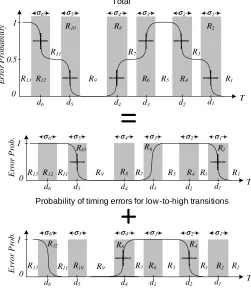
Figure 4 demonstrates the measured probability of timing error with respect to T in the top plot. Inequality 13 drives the pattern seen in regionR5. The metastability in inequality
14 is reflected in regionsR6 andR8. The error-free area R9
corresponds to Inequality 15. Regions R3, R7 and R11 are
results of the difference between tl→h
p and tlp→h. Inequality
16 is reflected in regions R10 and R12. Lastly, region R13
depicts the Equation 17.
Note that all the delays defined in this section, i.e., for the FFs, clock skews, and XOR, shall have two different values for the rising and falling edge transitions. The inequalities defined in this section hold for both rising and falling transitions.
T 1
0 0.5
σ6 σ5 σ4 σ3 σ2 σ1
d6 d5 d4 d3 d2 d1
R1 R3 R12 R2 R4 R5 R6 R7 R8 R9 R10 R11 R13 E r ro r P ro b a b il it y T 0
1 σ6 σ5 σ4 σ3 σ2 σ1
d6 d5 d4 d3 d2 d1
R1 R3 R12 R2 R4 R5 R6 R7 R8 R9 R10 R11 R13 T 0
1 σ6 σ5 σ4 σ3 σ2 σ1
d6 d5 d4 d3 d2 d1
R1 R3 R12 R2 R4 R5 R6 R7 R8 R9 R10 R11 R13 E rr o r P ro b . E rr o r P ro b . Total
Probability of timing errors for low-to-high transitions
Probability of timing errors for high -to-low transitions
Fig. 4. Probability of incurring timing errors as a function of half clock period (T).
cellor simply acell. In our implementation, we place each cell in one configurable logic block (CLB) on FPGA.
B. Timing Characterization Method
We now describe the timing measurement system which efficiently extracts the probability of obtaining timing failure for various clock pulse widths on the FPGA. The circuit demonstrated in Figure 3 only generates a single bit flag indicating the presence or absence of an error. Our objective is to design a method to measure the rate or probability at which errors appear at the circuit output in Figure 3 to extract the transitions as discussed in Figure 4.
In order to measure the probability of error at a certain clock frequency, an error histogram accumulator is realized by two counters. The first one is an error counter whose value increments by one each time an error occurs. The second one counts the clock cycles and also after 2N clock cycles
clears (resets) the error counter and restarts again, where N is the binary counters’ size. The error counter value is stored in the memory one clock cycle before it is reset. Now, the stored number of flaws normalized toN would yield the error probability value.
Next, we linearly and continually sweep the input clock frequency: in Tsweep seconds from fi = 21T
i to ft =
1
2Tt,
where Tt < tp < Ti. For each frequency sweep a separate
set of registers count the number of clock pulses. We use this counter as an accurate timer which records the frequency of the timing errors. This counter value is retrieved every time
O R
OR Column Address Decoder
R ow A dd re ss D ec od er Error Counter Controller Global Clock Write Increment C el l A dd re ss Address Counter Clear
Clock pulse numberClock Pulse Counter
O R O R C ha lle ng e Momery Clear
Fig. 5. The architecture for chip level delay extraction of logic components.
the content of the error counter is written into memory. The value of this counter is retrieved every time the error counter content is written into memory.
The system described above is utilized for extracting the delays of any CUT implemented on FPGA. A logic config-uration can be used within the CUT in the characterization circuit. The delay of each CUT component can be found by sweeping the clock frequency once. Note that the scanning for extracting delay values could also be performed in parallel to reduce the characterization time .
C. Characterization Accuracy
The resolution of the delay measurement, i.e., the measured delay’s accuracy, is a function of a few factors: (i) the clock noise and skew, (ii) the sweeping frequency resolution, and (iii) the number of pulses at each frequency. The output of the characterization circuit is a binary zero/one value. A real-valued output can be measured by repeating several (same width) clock pulses to the circuitry and accumulating the number of ones at the output. The resulting value, when normalized, shows the probability at which the timing errors occur for each input clock’s pulse width. The more the input clock pulse is repeated, the higher sampling resolution and accuracy can be achieved.
Next, assume that the clock pulse (of widthT) is sent to the CUT for M times. Because of clock skew and phase noise, the characterization circuitry receives a clock pulse with width Tef f =T+Tj, whereTj is the additive jitter. Suppose that
Tj is a random variable with a zero mean and symmetric
distribution around its mean. The output probability is a con-tinuous and smooth function ofTef f; thus, approximating the
D. Parameter Extraction
Thus far, we have described a system that measures the probability of timing errors for various clock pulse widths. The error probability can be fully represented by a set of few parameters; the parameters are directly related to the CUT delay and FF setup and hold times. It can be shown that the probability of timing errors shall be written as the sum of shifted Gaussian CDFs. The central limit theorem can determine the Gaussian nature of the error probabilities which can be explained by Equation 18 shows the parameterized error probability function.
fD,Σ(t) = 1 + 0.5 |Σ∑|−1
i=1
−1⌈i/2⌉ [
Q(t−di σi
) ]
(18)
whereQ(x)=√1
2π
∫∞
x exp
( −u2
2 )
anddi+1> di. To estimate
the timing parameters, f is fit to the set of measured data points (ti,ei), where ei is the error value recorded when the
pulse width equals ti.
E. Side-channel timing analysis of XOR’ed outputs
The objective of the timing circuitry and measurement method (described above) is for providing additional infor-mation about the individual response bits (i.e., PUF output bits) even though the response bits are XOR’ed together for providing the output. Assume thatkresponse bits{r1, . . . , rk}
are XOR’ed to form a single output bito. (Note that a k-input XOR shall consist of several stages of smaller XOR gates. For the same of demonstration, assume that the delay of the response bit ri, denoted by tri follows a certain order, say
tr1 ≤tr2· · · ≤trk−1 ≤trk).
As we sweep the clock frequency (in a rising trend) to measure the XOR’ed response bit, we eventually get to a regime where the frequency of the sweeping clock is close to the overall output (after XOR’ing). However, before we get to that regime, there are clock periods for which only a few XOR inputs (i.e., response bits) change. Sweeping the clock frequency could yield the information about the approximate timing of the XOR inputs. Even though we would not be able to tell which of the response bits had changes, we shall, with a good probability, determine the number of flipping XOR inputs. This number shall be vague if the timings of two or more response bits coincide. Since the probability of such a coincidence is rather low, in most instances clock sweeping can give us an approximation of the number of flipped XOR inputs, i.e., on the cumulative number of zeros and ones among the single Arbiter PUF responsesr1, . . . , rk.
V. COMBININGOURSIDECHANNELINFORMATION WITH
MACHINELEARNINGTECHNIQUES
The question if (and how) the side channel information on the cumulative number of zeros and ones can be efficiently exploited in modeling attacks turned out to be non-trivial. The obvious problem is that this number does not indicate which
of the single Arbiter PUF outputs has been zero or one. In a first attempt to resolve the problem, we only used those CRPs where the side channel indicates that all single Arbiter
PUF outputs are one or that all are zero in the modeling process. In these cases, we obviously do know every single output. By collecting such “special” CRPs, the problem of modeling an entire Lightweight PUF decomposes into the problem of modeling single Arbiter PUFs, which is known to be simple, and can be done with a linear number of CRPs and an approximately quadratic computational complexity [32], [34]. However, one of several problems with this strategy is that the “special” CRPs are exponentially rare, and merely constitute a fraction of 1/2k−1 of all CRPs. One therefore needs to collect an exponential amount of CRPs to implement this strategy.
Finally, we found a gradient based optimization similar to the logistic regression (LR) algorithm that has been used in earlier ML attacks on the XOR Arbiter PUF and Lightweight PUF [32], [34], and which is described in Section II-B. The following treatment assumes some familiarity with this algorithm and with the work in [32], [34].
Let ri(C) ∈ {0,1} be the output of the ith Arbiter PUF
within a k-XOR Arbiter PUF (or within a Lightweight PUF with k parallel Arbiter PUFs) to a challenge C. The side channel information then yields the number n of individual Arbiter PUFs with output one: n = ∑iri(C). It lies in
contrast to the general setting of binary outputs in LR on an interval scale. Therefore, instead of optimizing the binary class probabilities Eqn. 2, we rely on minimizing the squared error between a side channel modelf(w, C⃗ )and the actual outputs n:
l(M, ⃗w) = ∑
(C, t)∈ M
(f(w, C⃗ )−n)2.
The corresponding gradient
∇l(M, ⃗w) = ∑
(C, r)∈ M
2 (f(w⃗)−n)∇f(w⃗) (19)
is highly similar to the gradient in LR (Eqn. 4) and we will again apply the RProp update scheme (as in [32], [34]) to find a solutionw⃗ˆ with minimal errorl.
Assuming the standard linear additive delay model (see Section II-C and Eqn. 5), one obtains the following model of the side channel information:
f(w, C⃗ ) =∑
i
Θ(w⃗TiΦ⃗i).
Note that the model only depends on the direction, but not on the length ∥w⃗i∥ of the weight vectors. That is, any two
solutions w⃗i and α ⃗wi, α ∈ R+ are equivalent. Therefore
we might substitute the Heaviside function by the differ-entiable logistic sigmoid σ(x) = (1 +e−x)−1 to enable
gradient based optimization. This is a reasonable substitution as lim∥w⃗∥→∞σ(w⃗TΦ) = Θ(⃗ w⃗T⃗Φ) and, as noted above, a
valid solution is unaffected by scaling of w⃗.
As this substitution makes the model differentiable, we obtain the following gradient to insert in Eqn. 19:
∇f(w⃗j) =σ(w⃗jTΦ⃗j)(1−σ(w⃗Tj⃗Φj))⃗Φj. (20)
This gradient of an individual Arbiter PUF’s weight vectorw⃗j
weight vectors w⃗i of all other Arbiter PUFs. The decoupling
of individual Arbiter PUF updates thus drastically simplifies the ML problem, provided that side channel information is available.
In addition to the above new regression, we applied a two step optimization methodology: First we optimized the PUF model based on the above process and gradient, using the side channel information, until a fraction of f = 0.95percent of the final XOR Arbiter output was correctly reproduced. Secondly, we further refined and optimized the model with the “standard” LR algorithm applied in [32], [34] for 1000 iterations. This led to very low error rates around 2% or below. For all experiments, we used hundred times more CRPs than free parameters in the model, i.e.,
NCRP ≈100×bitlength×no. of XORs.
Note that the above equation merely describes a linear CRP consumption in the problem parameters. This is in stark contrast to the exponentially growing complexities of pure machine learning attacks on XOR Arbiter and Lightweight PUFs (see Table I and [32], [34]).
While our above process in the first step of the above methodology mostly converged to the global minimum, in a few cases it got stuck (i.e., the performance after 5000 iterations was worse than 5% remaining missclassifications). In this case, we restarted the algorithm with a different random initialization of w⃗.
VI. RESULTS ONSIMULATEDCRPS
We now analyze the performance of our combined modeling and side channel technique on simulated, noise-free CRPs and side channels, as detailed in Section II. As discussed earlier, simulated CRPs generated by the linear additive delay model are very close to silicon CRPs of Arbiter PUF variants, as proven in [34]. A very detailed discussion on the use of simulated CRPs, PUF noise, and ML performance, which advocates and justifies the use of simulated CRPs in security analyses of any Arbiter PUF variants, is given Section II-G of R¨uhrmair et al. [34].
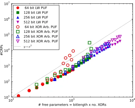
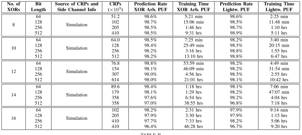
All results of our ML algorithms on simulated CRPs and side channel information are given as data points on a log-arithmic scale in Figure 6. They reach from 2 to 16 XORs with a stepwidth of 1, and concern 64, 128, 256 and 512 bits. For selected values, the detailed Figures are given in Table II. Note that the side channel information on the cumulative number of zeros and ones is the same for both our power and timing side channel. The results of the table therefore apply to both side channel approaches.
Table II and Figure 6 shows that the training times and CRP consumptions of our approach are remarkably small, especially compared to the exponentially growing complexities of pure machine learning attacks on XOR Arbiter and Lightweight PUFs (see Table I and [32], [34]). The number of CRPs that we used in all cases followed the earlier formula
NCRP ≈100×bitlength×no. of XORs.
The only exception were the cases of 14 XORs and 16 XORs for bitlengths 512, where our RAM was insufficient to carry
all CRPs. In these cases, we used50×bitlength×no. of XORs (see Table II). This led to slightly longer computation times, but did not prevent successful learning. Once more, this indicates the robustness of our method against small parameter changes.
We also thoroughly analyzed the training times of our algorithm. The results are illustrated on a logarithmic scale in Figure 6. The data shows that the computation times (=training times) are low-degree polynomial, presumably cubic, in the problem size (i.e., in the bitlengths and the number of XORs). Therefore our attacks can, in principle, be extended quite easily to larger PUF sizes. At the same time, the sizes of XOR-based Arbiter PUFs cannot be rised indefinitely: The practical instability of the XOR Arbiter PUF and the Lightweight PUF increases exponentially with the number of XORs, as already observed in [32], [34]. The two considered PUF designs hence can no longer be regarded secure without countermeasures in the presence of side channel attacks.
102 103 104
# free parameters = bitlength x no. XORs 101
102
103
104
105
106
107
#C
RP
s
64 bit LW PUF 128 bit LW PUF 256 bit LW PUF 512 bit LW PUF 64 bit XOR Arb. PUF 128 bit XOR Arb. PUF 256 bit XOR Arb. PUF 512 bit XOR Arb. PUF
y =x3
Fig. 6. The training times for our ML-algorithm on Lightweight PUFs (LW PUFs) and XOR Arbiter PUFs on a logarithmic scale. They show that the computational complexity regarding training times is cubic, i.e.,O(x3).
A final interesting effect is that with side channel informa-tion, the performance of our ML algorithms on Lightweight PUFs is slightly faster than for XOR Arbiter PUF, leading to smaller computation times. Without side channels, the converse effect has been observed [32], [34]. Intuitively, the challenge input mapping of the Lightweight PUF creates a more diverse and stable information basis for the ML algo-rithm, which leads to faster convergence. A full mathematical analysis of this effect will be conducted in future work.
VII. PROOF OFCONCEPT FORFPGA IMPLEMENTATIONS
A. Implementation of Lightweight PUFs and XOR Arbiter PUFs on FPGAs
No. of Bit Source of CRPs and CRPs Prediction Rate Training Time Prediction Rate Training Time XORs Length Side Channel Info (×103) XOR Arb. PUF XOR Arb. PUF Lightw. PUF Lightw. PUF
8
64
Simulation
51.2 98.6% 5:21 min 98.6% 2:25 min
128 102 98.7% 15:06 min 98.5% 11:48 min
256 205 98.5% 1:46 hrs 98.7% 1:10 hrs
512 410 98.5% 9:31 hrs 98.9% 5:11 hrs
10
64
Simulation
64.0 98.5% 7:25 min 98.2% 3:40 min
128 128 98.4% 25:49 min 98.5% 20:15 min
256 256 98.2% 3:16 hrs 98.8% 1:55 hrs
512 512 98.2% 13:10 hrs 98.8% 6:47 hrs
12
64
Simulation
76.8 98.8% 53:59 min 98.2% 4:49 min
128 154 98.1% 46:09 min 98.2% 31:54 min
256 307 98.0% 4:56 hrs 98.5% 2:55 hrs
512 614 98.0% 21:01 hrs 98.1% 10:42 hrs
14
64
Simulation
89.6 98.4% 1:18 hrs 98.1% 7:06 min
128 179 98.1% 1:29 hrs 98.2% 47:07 min
256 358 97.6% 6:54 hrs 98.2% 4:04 hrs
512 358 97.0% 38:55 hrs 96.8% 7:18 hrs
16
64
Simulation
102 98.2% 2:31 hrs 97.9% 9:14 min
128 205 97.9% 3:30 hrs 97.9% 1:15 hrs
256 410 97.7% 7:33 hrs 98.2% 5:06 hrs
512 410 96.4% 46:28 hrs 96.7% 9:20 hrs
TABLE II
PERFORMANCE OF COMBINED MODELING AND SIDE CHANNEL ATTACKS ONXOR ARBITERPUFS ANDLIGHTWEIGHTPUFS. ALL SHOWN RESULTS WERE OBTAINED ON SIMULATEDCRPS GENERATED BY THE ADDITIVE LINEAR DELAY MODEL[13], [32], [34]. THE SIDE CHANNEL INFORMATION ON THE NUMBER OF ZEROS AND ONES BEFORE THEXORGATE IS SIMULATED AND NOISE-FREE,TOO;PLEASE NOTE THAT IT IS THE SAME FOR POWER AND
TI MING SIDE CHANNELS(NAMELY THE CUMULATIVE NUMBER OF ZEROS AND ONES BEFORE THEXORGATE).
in Figure 1. In order to balance FPGA routing asymmetries, which would otherwise dominate the effect of manufacturing variations, a lookup table (LUT) based Programmable Delay Line (PDL) has been implemented, as in Figure7, as suggested by Majzoobi et al. [18], [15].
A1
1
1
1
1 0 0 0 0
A2 A3 SRAM
VALUE
OUT
3-input LUT
A2 A3
A1 OUT
3-input LUT A3
A2
A1
OUT
v
t
v
t tA
v
t tB
Fig. 7. LUT based Programmable Delay Line
For each CRP, majority voting over five repeated measure-ments of the response to the same challenge was performed in order to determine the final response. For example, if the five measurements resulted in three ”0”s and two ”1”s, the final response was set to ”0”. The challenges were generated by aN-bit pseudorandom number generator (PRNG), which
was based on a maximal-length linear feedback shift register (LFSR). The chosen LFSR polynomial generated the maximal-length sequence according to Eqn. 21:
F = 1 +X1+X3+X4+X64 (21)
B. Implementation of the Timing Side Channel Measurements
We executed the timing measurements of Section IV on our PUF implementations on Digilent Spartan 6 FPGAs of Section VII-A. Both XOR Arbiter PUFs and Lightweight PUF with 8 XORs and bitlengths 64, 128, 256 and 512 were built. For delay signature extraction, designed PUF circuits are utilized as the CUT part in Figure 3. For each CRP, we collected both side channel info on the cumulative number of ones and zeros, as well as the “global” responseo of the PUF after the final XOR gate. The latter response was stabilized by repeating the CRP measurement five times, and by applying majority voting (see above). As indicated above, in most instances clock sweeping only gives us an approximation of the number of flipped XOR inputs (i.e., of the cumulative ones and zeros).
No. of Bit Source of CRPs and CRPs Prediction Rate Training Time Prediction Rate Training Time XORs Length Side Channel Info (×103) XOR Arb. PUF XOR Arb. PUF Lightw. PUF Lightw. PUF
8
64
FPGA
26 98.5% 2 min 98.5% 1 min
128 51.6 97.5% 12 min 98.2% 9 min
256 103 97.7% 1:35 hrs 97.8% 1:00 hrs
512 205 97.4% 16:50 hrs 97.5% 3:30 hrs
12
64
FPGA
39 98.1% 16.5 min 98.5% 2 min
128 77.4 97.4% 38.5 min 97.9% 24.1 min
256 154.5 97.1% 3.8 hrs 97.3% 1.75 hrs
512 308 96.92% 56.25 hrs 97.11% 9.55 hrs
16
64
FPGA
52 98% 37 min 98% 7 min
128 103.2 97.5% 2 hrs 97.5% 51.7 min
256 206 97.3% 15.1 hrs 96.9% 4.8 hrs
512 410 96.5% 102 hrs 96.7% 20.2 hrs
TABLE III
FULL EXPERIMENTAL PROOF OF CONCEPT OF COMBINED MODELING AND TIMING SIDE CHANNEL ATTACKS,CARRIED OUT ONFPGA IMPLEMENTATIONS OF THEXOR ARBITERPUFANDLIGHTWEIGHTPUF.
C. Results
We applied our adapted ML algorithms of Section V to sili-con CRP data collected from the above FPGA implementation of Lightweight PUFs and XOR Arbiter PUFs, using silicon side channel information collected directly from these FPGAs (see Sections VII-B and VII).
Our approach led to the results shown in Table III. There is very little performance loss compared to the results for 8 XORs and bitlengths 64, 128, 256, and 512 on simulated data (see Table II). The number of used CRPs followed the formula 50×bitlength×no. of CRPs, i.e., we only used half as many CRPs as in the silicon case. The good results shows the robustness of our method, and indicate the efficiency of our above measures for the error-free collection of CRPs and associated side channel info. They also settle once more the viability of ML results on simulated CRPs, which was already postulated and confirmed in earlier work [32], [34], even for very large number of XORs and bitlengths, and even in the presence of side channel information. Our result breaks “real”, silicon FPGA implementations of 8 XOR Arbiter PUFs with bitlengths up to 512. The latter construction had been explicitly suggested as secure against pure modeling approaches in earlier work [32], [34].
VIII. COUNTERMEASURES
A. Countermeasures against our Power Side Channel
In order to immunize arbiter-based PUFs against power tracking SCA, one could add an additional, symmetric arbiter at the last stage of the PUF. The input signal for the added arbiter is inverted before it enters the arbiter (see Figure 8).
This idea behind the architecture is obviously to keep the number of zeros and ones in the entire PUF architecture con-stant, thereby preventing power tracking side channel attacks. A differential output of the described kind could also be desirable in fault tolerant applications, since it might allow error correction, and indicate unstable responses. Recall that the arbiter (=latch element) typically is one of the main sources of instability in an arbiter PUF: Signal pathes with a runtime difference that is on the order of the switching time of the latch often cause unstable responses. If the two differential
b1 b2 b3 bn-1 bn
Fig. 8. Standard Arbiter PUF with a differential output. Two arbiters are employed to generate two differential response bits, which have inverted input signals. The architecture would prevent the use of power tracking SCA. Asides, it also provides new error detection and correction capabilities.
latches have inconsistent content, this indicates the occurence of an unstable PUF response.
Use of k latches in such a differential design, together with standard majority voting over the latches’ outputs, could be used as a simple and very efficient means for response stabilization and error correction. We did not work out this idea in detail, however, since it is not within the main scope of this paper.
B. Countermeasures againt our Timing Side Channel
The timing side channel attacks depend on the correlations between the secret and the information leaked through the side channels. Several different countermeasures appear possible. For example, it is possible to jam the leaked timing side-channel with random pulses after the XOR so the attacher is not able to find the exact switching time of the XOR gates. Another plausible countermeasure is to place XOR/XNOR devices such that every time we get exactly one of them switching so it is hard to know which of the signal directions was the legitimate one.
constant delay (lower bounded by the 99% maximum PUF and XOR line delay. (Recall that the AND gate switches only if both of its inputs are ’1’.) The constant delay is generated by a line of buffers. The output of this line is fed into the second port of the AND gate. (Care shall be taken to equalize the routing to all the AND gates.) Now, the outputs of the AND gates will all switch simultaneously (or within a short time interval based on the AND gate process variations). In this way, the timing of output of the XOR gates shall be constant and (mostly) no-leaking information about the internal values before the XOR gates.
IX. SUMMARY ANDCONCLUSIONS
In this paper, we investigated the reach of combined mod-eling and side channel attacks on electrical Strong PUFs architectures. We exemplified our attacks on XOR Arbiter PUFs and Lightweight PUFs, since they are considered two of the most secure electrical Strong PUF architectures [32], [34]. Previous works had found that these two PUFs could only be attacked successfully for up to five or six XORed single Arbiter PUFs, and for bitlengths of 64 bits or 128 bits [32], [34], by the state of the art in pure modeling attacks. XOR Arbiter PUFs or Lightweight PUFs with bitlenghts of 512 and eight single Arbiter PUFs had explicitly been suggested as both practical (i.e., sufficiently stable) and fully secure in earlier works [32], [34].
The two side channels we have suggested and examined in this work were power tracing of the arbiter element (i.e., the latch) in Arbiter PUFs and variants thereof, and marking different response patterns with corresponding timing signa-tures. These are the first power and timing side channels for PUFs reported in the literature. Both tell us the cumulative number of zeros and ones in the outputs of the k parallel Arbiter PUFs within an XOR Arbiter PUF or Lightweight Arbiter PUF structure. Taken by itself, this side channel info is almost worthless, since the attacker does not learnwhichof the single Arbiter PUF outputs is zero or one. As we showed in this paper, however, it is possible to adapt existing ML techniques in such a way that they can efficiently exploit this simple side channel information. This adaption turned out to be non-trivial, and constitutes one of the main contributions of this paper.
It very strongly boosts ML performance, and reduces the ML training complexity and CRP consumption on the above two PUFs from exponential [32], [34] to an empirically estimated low degree polynomial in this work. Without coun-termeasures against our side channels, the two above PUFs can hence no longer be regarded secure: Their practical instability increases exponentially in the number of XORs [32], [34], while the attack complexity (or security) rises only low-degree polynomial in this parameter.
Firstly, we attacked XOR Arbiter PUFs and Lightweight PUFs for up to 16 XORs and bitlengths of up to 512 on simulated side channel info and CRPs (see Table II). The use of simulated data poses no very strong restriction on our results: Earlier investigations had shown that simulated CRPs are very close to silicon CRPs, and had explicitly
suggested that they can be used very well in any security analyses of Arbiter PUFs variants [34]. Furthermore, the error tolerance of our ML algorithms has been demonstrated in [32], [34], meaning that results obtained on error-free side channels should carry over well to the silicon case. Please note that the use of simulated data was an necessary step in order to conduct a large number of ML experiments, and to empirically estimate the complexity of our attacks on a sound basis.
Secondly, we carried out a full proof of concept for model-ing and timmodel-ing side channel attacks on FPGA implementations of the XOR Arbiter PUF and the Lightweight PUF (see Table III). They indeed confirmed that our results on simulated data carry over with little performance loss to the silicon case. The sizes and complexities we attacked successfully were 8 XORs and 12 XORs with 64, 128, 256, and 512 bits. One reason for choosing these specific sizes was that at CCS 2010 and IEEE T-IFS 2013 [32], [34], 8 XORs with bitlength 512 had been been suggested explicitly in theory as both practical (i.e., stable) and secure against pure modeling attacks. We stress that comparable sizes of the above two PUF types has never been implemented in silicon prior to our work. We implemented them for the first time, and subsequently tackled them successfully by our new attack method.
Finally, we discussed countermeasures against our side channels. They could and should be put in place in order to secure future Arbiter PUF generations against this method. Our countermeasure against the power side channel consists of using two symmetric, inverted output signals with two latches. This construction neutralizes and balances power consumption, regardless of PUF’s output. Interestingly, it can also be used to detect and stabilize output errors in Arbiter PUF variants, even though we did not work out this possibility in detail in this paper. We also discussed some countermeasure against our timing side channels, focusing on the construction of an isochronous hardware.
The PUF-attacks presented in this and other recent papers could be seen as a natural consolidation process in the PUF area, similar to the detailed investigations that classical cryptoprimitives and security systems have already undergone in the last decades. We believe that this interplay between attacks and countermeasures in the long term might well be beneficial for PUFs. Similar as in the case of classical security systems, it could eventually lead to improved PUF designs and implementations, which withstand all known attack forms at some point.
INDIVIDUALCONTRIBUTIONS OF THEAUTHORS