Study And Comparison Of Various Mppt Algorithms In Solar Power System

ISSN 2348 – 7968

Study and Comparison of Various MPPT Algorithms in Solar Power

System

AnuradhaP 1

P

and Satish Kumar P 2

P

P

1

P

Electrical Engineering Department, RPIIT, Karnal, Haryana 132001, India

P

2

P

Electrical Engineering Department, RPIIT, Karnal, Haryana 132001, India

Abstract— Several techniques for MPPT (maximum power point tracking of photovoltaic (PV) arrays have been proposed. A vast literature survey starting from the earliest method is summarized in this paper. These techniques are taken from the literature dating back to the earliest methods. A comparative analysis of these different techniques can be taken as reference for the future work on solar power generation.

Index Terms—MPPT, PV panel, Solar Power..

I. INTRODUCTION

Maximum power point in solar or PV power generation gives the best possible efficiency of the PV-panel. MPPT driven by a particular technique track the maximum power point (MPP) of a photovoltaic (PV) array. Tracking is usually an essential part of a PV system. As such, many MPP tracking (MPPT) methods have been developed and implemented. The methods vary in complexity, sensors required, convergence speed, cost, range of effectiveness, implementation hardware, popularity, and in other respects. They range from the almost obvious (but not necessarily ineffective) to the most creative (not necessarily most effective). In fact, so many methods have been developed that it has become difficult to adequately determine which method, newly proposed or existing, is most appropriate for a given PV system. Given the large number of methods for MPPT, a survey of the methods would be very beneficial to researchers and practitioners in PV systems.

The focus on research work on this area per year has grown considerably of the last decades and remains strong. However, recent papers have generally had shorter, more cursory literature reviews that largely summarize or repeat the literature reviews of previous work. This approach tends to repeat what seems to be conventional wisdom that there are only a handful of MPPT techniques, when in fact there are many. This is due to the sheer volume of MPPT literature to review, conflicting with the need for brevity.

In this paper, the attention will be focused on experimental comparisons between some of these techniques, considering several irradiation conditions. Therefore, the aim of this work is to compare several widely adopted MPPT algorithms between them in order to understand which technique has the best performance. The evaluation of the algorithms’ performance is based on the power measurement valuating the total energy produced by the panel during the same test cycle. In this work, respect to the MPPT algorithm compared by simulations, the methods that need temperature or irradiance measure-ments are not considered for sake of simplicity. Indeed, as described in [11], these techniques do not have very high performance and they are too expensive. In the simulations, the considered MPPT techniques have been implemented strictly following the description indicated in the references: no MPPT algorithm is preferred and no MPPT techniques have been realized with more attention respect to the others.

II. PROBLEM OVERVIEW

Fig. 1 shows the characteristic power curve for a PV array. The problem considered by MPPT techniques is to automatically find the voltage VMPP or current

IMPP at which a PV array should operate to obtain the

maximum power output PMPP under a given

temperature and irradiance. It is noted that under partial shading conditions, in some cases it is possible to have multiple local maxima, but overall there is still only one true MPP. Most techniques respond to changes in both irradiance and temperature, but some are specifically more useful if temperature is approximately constant. Most techniques would automatically respond to changes in the array due to aging, though some are open-loop and would require periodic fine-tuning. In our context, the array will typically be connected to a power converter that can vary the current coming from the PV array.

Fig. 1. Characteristic PV array power curve.

TABLE I

SUMMARY OF HILL CLIMBING AND P&O ALGORITHM

III. MPPT TECHNIQUES

We introduce the different MPPT techniques below in an arbitrary order.

A. Hill Climbing/P&O

Among all the papers we gathered, much focus has been on hill climbing [1]–[8], and perturb and observe (P&O) [9]–[25] methods. Hill climbing involves a perturbation in the duty ratio of the power converter, and P&O a perturbation in the operating voltage of the PV array. In the case of a PV array connected to a power converter, perturbing the duty ratio of power converter perturbs the PV array current and consequently perturbs the PV array voltage. Hill climbing and P&O methods are different ways to envision the same fundamental method. From Fig. 1, it can be seen that incrementing (decrementing) the voltage increases (decreases) the power when operating on the left of the MPP and decreases (increases) the power when on the right of the MPP. Therefore, if there is an increase in power, the subsequent perturbation should be kept the same to reach the MPP and if there is a decrease in power, the perturbation should be reversed. This algorithm is summarized in Table I. In [24], it is shown that the algorithm also works when instantaneous (instead of average) PV array voltage and current are used, as long as sampling occurs only once in each switching cycle. The process is repeated periodically until the MPP is reached. The system then oscillates about the MPP. The oscillation can be minimized by reducing the perturbation step size. However, a smaller perturbation size slows down the MPPT. A solution to this conflicting situation is to have a variable perturbation size that gets smaller towards the MPP as shown in [8], [12], [15], and [22]. In [24], fuzzy

logic control is used to optimize the magnitude of the next perturbation. In [20], a two-stage algorithm is proposed that offers faster tracking in the first stage.

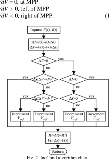
B. Incremental Conductance

The incremental conductance (IncCond) [9], [26]– [36] method is based on the fact that the slope of the PV array power curve (Fig. 1) is zero at the MPP, positive on the left of the MPP, and negative on the right, as given by

dP/dV = 0, at MPP dP/dV > 0, left of MPP

dP/dV < 0, right of MPP. (1)

Fig. 2. IncCond algorithm chart.

The MPP can thus be tracked by comparing the instantaneous conductance (I/V ) to the incremental conductance (ΔI/ΔV ) as shown in the flowchart in Fig. 2. Vref is the reference voltage at which the PV array is forced to operate. At the MPP, Vref equals to

the open-circuit voltage (VOC) to the short-circuit current (ISC) of the PV array. This two-stage alternative also ensures that the real MPP is tracked in case of multiple local maxima.

C. Fractional Open-Circuit Voltage

The near linear relationship between VMPP and VOC of the PV array, under varying irradiance and temperature levels, has given rise to the fractional

VOC method [30]–[35]. As VMPP ≈ k1VOC, where k1 is

a constant of proportionality. Since k1 is dependent

on the characteristics of the PV array being used, it usually has to be computed beforehand by empirically determining VMPP and VOC for the specific PV array at different irradiance and temperature levels. The factor k1 has been reported to be between 0.71 and 0.78. Once k1 is known, VMPP can be computed using VOC measured periodically by momentarily shutting down the power converter. However, this incurs some disadvantages, including temporary loss of power. To prevent this, [20] uses pilot cells from which VOC can be obtained. These pilot cells must be carefully chosen to closely represent the characteristics of the PV array. In [14], it is claimed that the voltage generated by pn-junction diodes is approximately 75% of VOC. This eliminates the need for measuring VOC and computing VMPP. Once VMPP has been approximated, a closed-loop control on the array power converter can be used to asymptotically reach this desired voltage. This computes only an approximation; the PV array technically never operates at the MPP. Depending on the application of the PV system, this can sometimes be adequate. Even if fractional VOC is not a true MPPT technique, it is very easy and cheap to implement as it does not necessarily require DSP or microcontroller control. However, [5] points out that k1 is no more valid in the presence of partial shading

(which causes multiple local maxima) of the PV array and proposes sweeping the PV array voltage to update k1. This obviously adds to the implementation

complexity and incurs more power loss.

D. Fractional Short-Circuit Current

Fractional ISC results from the fact that, under

varying atmospheric conditions, IMPP is

approximately linearly related to the

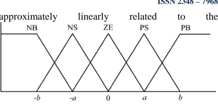
Fig. 3. Membership function for inputs and output of fuzzy logic controller.

ISC of the PV array as shown in [24 IMPP ≈ k2ISC, where k2 is a proportionality constant. Just like in the

fractional VOC technique, k2 has to be determined according to the PV array in use. The constant k2 is

generally found to be between 0.78 and 0.92.

Measuring ISC during operation is problematic. An additional switch usually has to be added to the power converter to periodically short the PV array so that ISC can be measured using a current sensor. This increases the number of components and cost. In [18], a boost converter is used, where the switch in the converter itself can be used to short the PV array. Power output is not only reduced when finding ISC but also because the MPP is never perfectly matched

as IMPP ≈ k2ISC. In [16], a way of compensating k2 is

proposed such that the MPP is better tracked while atmospheric conditions change. To guarantee proper MPPT in the presence of multiple local maxima, [15] periodically sweeps the PV array voltage from open-circuit to short-open-circuit to update k2. Most of the PV systems using fractional ISC in the literature use a DSP. In [28], a simple current feedback control loop is used instead.

E. Fuzzy Logic Control

levels as in [9] the inputs to a MPPT fuzzy logic controller are usually an error E and a change in error

ΔE. The user has the flexibility of choosing how to compute E and ΔE. Since dP/dV vanishes

TABLE II

FUZZY RULE BASE TABLE AS SHOWN IN [50]

at the MPP, [8] uses the approximation E(n) = P(n) − P(n − 1)

V (n) − V (n − 1) (2) and

ΔE(n) = E(n) − E(n − 1). (3)

Once E and ΔE are calculated and converted to the linguistic variables, the fuzzy logic controller output, which is typically a change in duty ratio ΔD of the power converter, can be looked up in a rule base table such as Table II [30]. The linguistic variables assigned to ΔD for the different combinations of E and ΔE are based on the power converter being used and also on the knowledge of the user. Table II is based on a boost converter. If, for example, the operating point is far to the left of the MPP (Fig. 1), that is E is PB, and ΔE is ZE, then we want to largely increase the duty ratio that is ΔD should be PB to reach the MPP. In the defuzzification stage, the fuzzy logic controller output is converted from a linguistic variable to a numerical variable still using a membership function as in Fig. 3. This provides an analog signal that will control the power converter to the MPP. MPPT fuzzy logic controllers have been shown to perform well under varying atmospheric conditions. However, their effectiveness depends a lot on the knowledge of the user or control engineer in choosing the right error computation and coming up with the rule base table. In [6], an adaptive fuzzy logic control is proposed that constantly tunes the membership functions and the rule base table so that optimum performance is achieved. Experimental results from [21] show fast convergence to the MPP and minimal fluctuation about it. In [27], two different membership functions are empirically used to show that the tracking performance depends on the type membership functions considered.

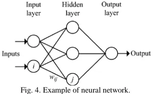
F. Neural Network

Along with fuzzy logic controllers came another technique of implementing MPPT—neural networks [10]–[13], which are also well adapted for microcontrollers. Neural networks commonly have three layers: input, hidden, and output layers as shown in Fig. 4. The number of nodes in each layer varies and is user-dependent. The input variables can be PV array parameters like VOC and ISC, atmospheric data like irradiance and temperature, or any combination of these.

Fig. 4. Example of neural network.

How close the operating point gets to the MPP depends on the algorithms used by the hidden layer and how well the neural network has been trained. The links between the nodes are all weighted. The link between nodes i and j is labeled as having a weight of wij in Fig. 4. To accurately identify the MPP, the wij ’s have to be carefully determined through a training process, whereby the PV array is tested over months or years and the patterns between the input(s) and output(s) of the neural network are recorded.

Since most PV arrays have different characteristics, a neural network has to be specifically trained for the PV array with which it will be used. The characteristics of a PV array also change with time, implying that the neural network has to be periodically trained to guarantee accurate MPPT.

G. RCC

When a PV array is connected to a power converter, the switching action of the power converter imposes voltage and current ripple on the PV array. As a consequence, the PV array power is also subject to ripple. Ripple correlation control (RCC) [28] makes use of ripple to perform MPPT

literature that use MPPT methods that resemble RCC. For example, [6] integrates the product of the signs of the time derivatives of power and of duty ratio. However, unlike RCC, which uses inherent ripple present in current and voltage, [9] disturbs the duty ratio to generate a disturbance in power. In [66] and [7], a hysteresis-based version of RCC is used. A low frequency dithering signal is used to disturb the power in [6]. In [68], a 90◦ phase shift in the current (or voltage) with respect to power at the MPP is discussed, just like in RCC. The difference in [8] is that the injection is an extra, low-frequency signal and not an inherent converter ripple.

H. Current Sweep

The current sweep [9] method uses a sweep waveform for the PV array current such that the I–V characteristic of the PV array is obtained and updated at fixed time intervals. The VMPP can then be computed from the characteristic curve at the same intervals.

Fig. 5. Topology for dc-link capacitor droop control as shown in

Once VMPP is computed after the current sweep, (17) can be used to double check whether the MPP has been reached. In [9], the current sweep method is implemented through analog computation. The current sweep takes about 50 ms, implying some loss of available power. In [69], it is pointed out that this MPPT technique is only feasible if the power consumption of the tracking unit is lower than the increase in power that it can bring to the entire PV system.

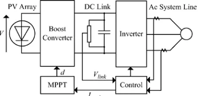
I. DC-Link Capacitor Droop Control

DC-link capacitor droop control [10], [11] is an MPPT technique that is specifically designed to work with a PV system that is connected in parallel with an ac system line as shown in Fig. 6.

Fig. 6. Topology for dc-link capacitor droop control as shown in [71].

the current going in the inverter increases the power coming out of the boost converter and consequently increases the power coming out of the PV array. While the current is increasing, the voltage Vlink can be kept constant as long as the power required by the inverter does not exceed the maximum power available from the PV array. If that is not the case, Vlink starts drooping. Right before that point, the current control command Ipeak of the inverter is at its maximum and the PV array operates at the MPP. The ac system line current is fed back to prevent Vlink from drooping and d is optimized to bring Ipeak to its maximum, thus achieving MPPT. DC-link capacitor droop control does not require the computation of the PV array power, but according to [12], its response deteriorates when compared to a method that detects the power directly; this is because its response directly depends on the response of the dc-voltage control loop of the inverter. This control scheme can be easily implemented with analog operational amplifiers and decision-making logic units.

Fig. 7. Different load types. 1: voltage source, 2: resistive, 3: resistive and voltage source, 4: current source, as shown in [78].

This is also true for nonlinear load types as long as they do not exhibit negative impedance characteristics. Therefore, for almost all loads of interest, it is adequate to maximize either

the load current or the load voltage to maximize the load power. Consequently, only one sensor is needed. In most PV systems, a battery is used as the main load or as a backup. Since a battery can be thought of as a voltage-source type load, the load current can be used as the control variable. In [13], [14], and [16], positive feedback is used to control the power converter such that the load current is maximized and the PV array operates close to the MPP. Operation exactly at the MPP is almost never achieved because this MPPT method is based on the assumption that the power converter is lossless.

K. dP/dV or dP/dI Feedback Control

With DSP and microcontroller being able to handle complex computations, an obvious way of performing MPPT is to compute the slope (dP/dV or dP/dI) of the PV power curve (Fig. 2) and feed it back to the power converter with some control to drive it to zero. This is exactly what is done in [9]– [5]. The way the slope is computed differs from paper to paper. In [9], dP/dV is computed and its sign is stored for the past few cycles. Based on these signs, the duty ratio of the power converter is either incremented or decremented to reach the MPP. A dynamic step size is used to improve the transient response of the system. In [80], a linearization-based method is used to compute dP/dV. In [21]–[23], sampling and data conversion are used with subsequent digital division of power and voltage to approximate dP/dV. In [22], dP/dI is then integrated together with an adaptive gain to improve the transient response. In [23], the PV-array voltage is periodically incremented or decremented and ΔP/Δ

V is compared to a marginal error until the MPP is reached. Convergence to the MPP was shown to occur in tens of milliseconds in [21].

L. Other MPPT Techniques

Other MPPT techniques include array reconfiguration [4], whereby PV arrays are arranged in different series and parallel combinations such that the resulting MPPs meet specific load requirements. This method is time consuming and tracking MPP in real time is not obvious. In [3], a linear current control is used based on the fact that a linear relationship exists between IMPP and the level of irradiance. The current

also needed. The maximum error in using LRCM to approximate the MPP was found to be 0.3%, but this was based only on simulation results. In [31], a slide control method with a buck-boost converter is used to achieve MPPT.

This control was implemented using a microcontroller that senses the PV array voltage and current. Simulation and experimental results showed that operation converges to the MPP in several tens of milliseconds.

IV. DISCUSSION

With so many MPPT techniques available to PV system users, it might not be obvious for the latter to

choose which one better suits their application needs. The main aspects of the MPPT techniques to be taken into consideration are highlighted in the following subsections.

A. Implementation

The ease of implementation is an important factor in deciding which MPPT technique to use. However, this greatly depends on the end-users’ knowledge. Some might be more familiar with analog circuitry, in which case, fractional ISC or VOC, RCC, and load current or voltage maximization are good options. Others might be willing to work with digital circuitry, even if that

TABLE III

MAJOR CHARACTERISTICS OF MPPT TECHNIQUES

may require the use of software and programming. Then, their selection should include hill climbing/P&O, IncCond, fuzzy logic control, neural network, and dP/dV or dP/dI feedback control. Furthermore, a few of the MPPT techniques only apply to specific topologies. For example, the dc-link capacitor droop control works with the system shown in Fig. 7 and the OCC MPPT works with a single-stage inverter.

B. Sensors

The number of sensors required to implement MPPT also affects the decision process. Most of the time, it is easier and more reliable to measure voltage than current. Moreover, current sensors are usually expensive and bulky. This might be inconvenient in systems that consist of several PV arrays with separate MPP trackers. In such cases, it might be wise to use MPPT methods that require only one sensor or that can estimate the current from the

voltage as in [25]. It is also uncommon to find sensors that measure irradiance levels, as needed in

the linear current control and the IMPP and VMPP computation methods.

C. Multiple Local Maxima

D. Costs

It is hard to mention the monetary costs of every single MPPT technique unless it is built and implemented. This is unfortunately out of the scope of this paper. However, a good costs comparison can be made by knowing whether the technique is analog or digital, whether it requires software and programming, and the number of sensors. Analog implementation is generally cheaper than digital, which normally involves a microcontroller that needs to be programmed. Eliminating current sensors considerably drops the costs.

E. Applications

Different MPPT techniques discussed earlier will suit different applications. For example, in space satellites and orbital stations that involve large amount of money, the costs and complexity of the MPP tracker are not as important as its performance and reliability. The tracker should be able to continuously track the true MPP in minimum amount of time and should not require periodic tuning. In this case, hill climbing/P&O, IncCond, and RCC are appropriate. Solar vehicles would mostly require fast convergence to the MPP. Fuzzy logic control, neural network, and RCC are good options in this case. Since the load in solar vehicles consists mainly of batteries, load current or voltage maximization should also be considered. The goal when using PV arrays in residential areas is to minimize the payback time and to do so, it is essential to constantly and quickly track the MPP. Since partial shading (from trees and other buildings) can be an issue, the MPPT should be capable of bypassing multiple local maxima. Therefore, the two-stage IncCond [31], [35] and the current sweep methods are suitable. Since a residential system might also include an inverter, the OCC MPPT can also be used. PV systems used for street lighting only consist in charging up batteries during the day. They do not necessarily need tight constraints; easy and cheap implementation might be more important, making fractional VOC or ISC viable.

For all other applications not mentioned here, we put together Table III, containing the major characteristics of all the MPPT techniques. Table III should help in choosing an appropriate MPPT method.

V. CONCLUSION

Several MPPT techniques taken from the literature are discussed and analyzed herein, with their pros and cons. It is shown that there are several other MPPT techniques than those commonly included in literature reviews. The concluding discussion and table should serve as a useful guide in choosing the right MPPT method for specific PV systems.

REFERENCES

[1] L. L. Buciarelli, B. L. Grossman, E. F. Lyon, and N. E. Rasmussen, “The energy balance associated with the use of aMPPT in a 100 kW peak power system,” in IEEE Photovoltaic Spec. Conf., 1980, pp. 523–527. [2] J. D. van Wyk and J. H. R. Enslin, “A study of wind power converter with microprocessor based power control utilizing an oversynchronous electronic scherbius cascade,” in Proc. IEEE Int. Power Electron. Conf., 1983, pp. 766–777.

[3] W. J. A. Teulings, J. C. Marpinard, A. Capel, and D. O’Sullivan, “A new maximum power point tracking system,” in Proc. 24th Annu. IEEE Power Electron. Spec. Conf., 1993, pp. 833–838.

[4] Y. Kim, H. Jo, and D. Kim, “A new peak power tracker for cost-effective photovoltaic power system,” in Proc. 31st Intersociety Energy Convers.Eng. Conf., 1996, pp. 1673–1678.

[5] O. Hashimoto, T. Shimizu, and G. Kimura, “A novel high performance utility interactive photovoltaic inverter system,” in Conf. Record 2000 IEEE Ind. Applicat. Conf., 2000, pp. 2255–2260.

[6] E. Koutroulis, K. Kalaitzakis, and N. C. Voulgaris, “Development of a microcontroller-based, photovoltaic maximum power point tracking control system,” IEEE Trans. Power Electron., vol. 16, no. 21, pp. 46– 54, Jan. 2001.

[7] M.Veerachary, T. Senjyu, andK.Uezato, “Maximum power point tracking control of IDB converter supplied PV system,” in IEE Proc. Elect. Power Applicat., 2001, pp. 494–502.

[8] W. Xiao and W. G. Dunford, “A modified adaptive hill climbing MPPT method for photovoltaic power systems,” in Proc. 35th Annu. IEEE Power Electron. Spec. Conf., 2004, pp. 1957–1963.

[9] O. Wasynczuk, “Dynamic behavior of a class of photovoltaic power systems,” IEEE Trans. Power App. Syst., vol. 102, no. 9, pp. 3031–3037, Sep. 1983.

[10] C. Hua and J. R. Lin, “DSP-based controller application in battery storage of photovoltaic system,” in Proc. IEEE IECON 22nd Int. Conf. Ind. Electron., Contr. Instrum., 1996, pp. 1705–1710.

[11] M. A. Slonim and L. M. Rahovich, “Maximum power point regulator for 4 kWsolar cell array connected through invertor to the AC grid,” in Proc. 31st Intersociety Energy Conver. Eng. Conf., 1996, pp. 1669–1672.

[12] A. Al-Amoudi and L. Zhang, “Optimal control of a grid-connected PV system for maximum power point tracking and unity power factor,” in Proc. Seventh Int. Conf. Power Electron. Variable Speed Drives, 1998, pp. 80–85.

[13] N. Kasa, T. Iida, and H. Iwamoto, “Maximum power point tracking with capacitor identifier for photovoltaic power system,” in Proc. Eighth Int. Conf. Power Electron. Variable Speed Drives, 2000, pp. 130–135. [14] L. Zhang, A. Al-Amoudi, and Y. Bai, “Real-time maximum power point tracking for grid-connected photovoltaic systems,” in Proc. Eighth Int. Conf. Power Electronics Variable Speed Drives, 2000, pp. 124–129. [15] C.-C. Hua and J.-R. Lin, “Fully digital control of distributed photovoltaic power systems,” in Proc. IEEE Int. Symp. Ind. Electron., 2001, pp. 1–6.

[16] M.-L. Chiang, C.-C. Hua, and J.-R. Lin, “Direct power control for distributed PV power system,” in Proc. Power Convers. Conf., 2002, pp. 311–315.

[17] K. Chomsuwan, P. Prisuwanna, and V. Monyakul, “Photovoltaic grid connected inverter using two-switch buck-boost converter,” in Conf. Record Twenty-Ninth IEEE Photovoltaic Spec. Conf., 2002, pp. 1527– 1530.

[18] Y.-T. Hsiao and C.-H. Chen, “Maximum power tracking for photovoltaic power system,” in Conf. Record 37th IAS Annu. Meeting Ind. Appl. Conf., 2002, pp. 1035–1040.

[21] T. Tafticht and K. Agbossou, “Development of a MPPT method for photovoltaic systems,” in Canadian Conf. Elect. Comput. Eng., 2004, pp. 1123– 1126.

[22] N. Femia, G. Petrone, G. Spagnuolo, and M. Vitelli, “Optimization of perturb and observe maximum power point trackingmethod,” IEEE Trans. Power Electron., vol. 20, no. 4, pp. 963–973, Jul. 2005.

[23] P. J. Wolfs and L. Tang, “A single cell maximum power point tracking converter without a current sensor for high performance vehicle solar arrays,” in Proc. 36th Annu. IEEE Power Electron. Spec. Conf., 2005, pp. 165–171.

[24] N. S. D’Souza, L. A. C. Lopes, and X. Liu, “An intelligent maximum power point tracker using peak current control,” in Proc. 36th Annu. IEEE Power Electron. Spec. Conf., 2005, pp. 172–177.

[25] N. Kasa, T. Iida, and L. Chen, “Flyback inverter controlled by sensorless currentMPPTfor photovoltaic power system,” IEEE Trans. Ind. Electron., vol. 52, no. 4, pp. 1145–1152, Aug. 2005.

[26] A. F. Boehringer, “Self-adapting dc converter for solar spacecraft power supply,” IEEE Trans. Aerosp. Electron. Syst., vol. AES-4, no. 1, pp. 102– 111, Jan. 1968.

[27] E. N. Costogue and S. Lindena, “Comparison of candidate solar array maximum power utilization approaches,” in Intersociety Energy Conversion Eng. Conf., 1976, pp. 1449–1456.

[28] J. Harada and G. Zhao, “Controlled power-interface between solar cells and ac sources,” in IEEE Telecommun. Power Conf., 1989, pp. 22.1/1–22.1/7.

[29] K. H. Hussein and I. Mota, “Maximum photovoltaic power tracking: An algorithm for rapidly changing atmospheric conditions,” in IEE Proc. Generation Transmiss. Distrib., 1995, pp. 59–64.

[30] A. Brambilla, M. Gambarara, A. Garutti, and F. Ronchi, “New approach to

photovoltaic arrays maximum power point tracking,” in Proc. 30th Annu. IEEE Power Electron. Spec. Conf., 1999, pp. 632–637.

[31] K. Irisawa, T. Saito, I. Takano, and Y. Sawada, “Maximum power point

tracking control of photovoltaic generation system under non-uniform insolation by means of monitoring cells,” in Conf. Record Twenty-Eighth IEEE Photovoltaic Spec. Conf., 2000, pp. 1707–1710.

[32] T.-Y. Kim, H.-G. Ahn, S. K. Park, and Y.-K. Lee, “A novel maximum power point tracking control for photovoltaic power system under rapidly changing solar radiation,” in IEEE Int. Symp. Ind. Electron., 2001, pp. 1011–1014.

[33] Y.-C. Kuo, T.-J. Liang, and J.-F. Chen, “Novel maximum-power-pointtracking controller for photovoltaic energy conversion system,” IEEE Trans. Ind. Electron., vol. 48, no. 3, pp. 594–601, Jun. 2001. [34] G. J. Yu, Y. S. Jung, J. Y. Choi, I. Choy, J. H. Song, and G. S. Kim, “A novel two-mode MPPT control algorithm based on comparative study of existing algorithms,” in Conf. Record Twenty-Ninth IEEE Photovoltaic Spec. Conf., 2002, pp. 1531–1534.

[35] K.Kobayashi, I. Takano, andY. Sawada, “A study on a two stagemaximum

power point tracking control of a photovoltaic system under partially shaded insolation conditions,” in IEEE Power Eng. Soc. Gen.Meet., 2003, pp. 2612–2617.