in the Dual-Solution Domain
Thesis by
Christopher A. Mouton
In Partial Fulfillment of the Requirements
for the Degree of
Doctor of Philosophy
California Institute of Technology
Pasadena, California
2007
c
2007
Christopher A. Mouton
Acknowledgements
I am sincerely grateful to my advisor, Dr. Hans Hornung, without whom none of this would
have been possible. He has given me so much room to grow and to explore my interest
in gas dynamics. His encouragement and guidance in all aspects of this work have been
invaluable to me, and are something I will never forget.
I am truly indebted to Bahram Valiferdowsi for his extensive help in the design,
manufac-ture, and repair of the Ludwieg tube facility. Without his expertise none of the experiments
presented in this thesis would have been possible. The work of John Korte of NASA Langley
Research Center on designing both the original Mach 2.3 as well as the Mach 4.0 is greatly
appreciated.
Nicolas Ponchaut has been an invaluable friend throughout my studies and research. He
has always been willing to assist me in my work, to criticize my math skills, to push me to
code more efficiently, and to discuss the many problems facing the world. He is truly one
of the smartest people I have met in my life, and I look up to him for that.
I would also like to thank the National Defense Science and Engineering Grant for
funding the first three years of my studies at Caltech. I also thank Dr. John Schmisseur
from the Air Force Office of Scientific Research for providing the funding and the trust to
pursue this study of Mach reflection.
A special thanks to Jeff Bergthorson, Jim Karnesky, Amy Lam, Stuart Laurence,
Daniel Lieberman, David Miller, Florian Pintgen, and Dr. Joseph Shepherd for giving me
advice or helping me with various tasks related to my experiments. Thanks to Julian
Cum-mings, Ralf Deiterding, and James Quirk for their help on the computational aspects of my
work. Thanks also to Joe Haggerty, Ali Kiani, Bradley St. John, and Ricardo Paniagua for
their work constructing many of the components of the Ludwieg tube facility.
Very importantly, I would like to thank my friends and family. The biggest thanks goes
and Paul, whose support and encouragement throughout my time at Caltech is something
I will always cherish. Thanks also to Damien for being an amazing friend and a perfect
business partner.
I greatly appreciate the inspiration and guidance of my previous professors and teachers:
Dr. David Goldstein, Jack McAleer, and Dr. Armando Galindo.
I also acknowledge the members of my committee: Dr. Hans Hornung, Dr. Joseph
Shep-herd, Dr. Dale Pullin, Dr. Paul Dimotakis, and Dr. Beverly McKeon for their suggestions
and for their time.
Abstract
A study of the shock-reflection domain for steady flow is presented. Conditions defining
boundaries between different possible shock-reflection solutions are given, and where
possi-ble, simple analytic expressions for these conditions are presented. A new, more accurate
estimate of the steady-state Mach stem height is derived based on geometric considerations
of the flow. In particular, the location of the sonic throat through which the subsonic
con-vergent flow behind the Mach stem is accelerated to dicon-vergent supersonic flow is considered.
Comparisons with previous computational and experimental work show that the theory
pre-sented in this thesis more accurately predicts the Mach stem height than previous theories.
The Mach stem height theory is generalized to allow for a moving triple point. Based on
this moving triple point theory, a Mach stem growth rate theory is developed. This theory
agrees well with computational and experimental results. Numerical computations of the
effects of water vapor disturbances are also presented. These disturbances are shown to be
sufficient to cause transition from regular reflection to Mach reflection in the dual-solution
domain. These disturbances are also modeled as a simple energy deposition on one of the
wedges, and an estimate for the minimum energy required to cause transition is derived.
Experimental results using an asymmetric wedge configuration in the Ludwieg tube
facility at the California institute of Technology are presented. A Mach 4.0 nozzle was
designed and built for the Ludwieg tube facility. This Mach number is sufficient to provide
a large dual-solution domain, while being small enough not to require preheating of the
test gas. The test time of the facility is 100 ms, which requires the use of high-speed
cine-matography and a fast motor to rotate one of the two wedges. Hysteresis in the transition
between regular to Mach reflection was successfully demonstrated in the Ludwieg tube
facil-ity. The experiments show that regular reflection could be maintained up to a shock angle
approximately halfway between the von Neumann condition and the detachment condition.
performed to measure the Mach stem height and its growth rate. These results are compared
with the theoretical estimates presented in this thesis. Excellent agreement between the
steady-state Mach stem height and the theoretical estimates is seen. Comparisons of Mach
stem growth rate with theoretical estimates show significant differences, but do show good
Contents
Acknowledgements v
Abstract vii
1 Introduction 1
1.1 Outline and Contributions . . . 6
2 Shock Reflection Domain 9 2.1 General Compressible Flow Equations . . . 9
2.2 Possible Shock Reflections . . . 11
2.2.1 Regular Reflection . . . 11
2.2.2 Regular Reflection with Subsonic Downstream Flow . . . 12
2.2.3 Mach Reflection . . . 12
2.2.4 Mach Reflection with Subsonic Downstream Flow . . . 13
2.2.5 Mach Reflection with a Forward-Facing Reflected Shock . . . 14
2.2.6 Inverted Mach Reflection . . . 14
2.2.7 Von Neumann Reflection . . . 15
2.3 Domain Boundaries . . . 17
2.3.1 Mach Wave Condition . . . 17
2.3.2 Sonic Incident Shock Condition . . . 17
2.3.3 Detachment Condition . . . 18
2.3.4 Von Neumann Condition . . . 22
2.3.5 Sonic Reflected Shock Condition . . . 26
2.3.6 Normal Reflected Shock Condition . . . 29
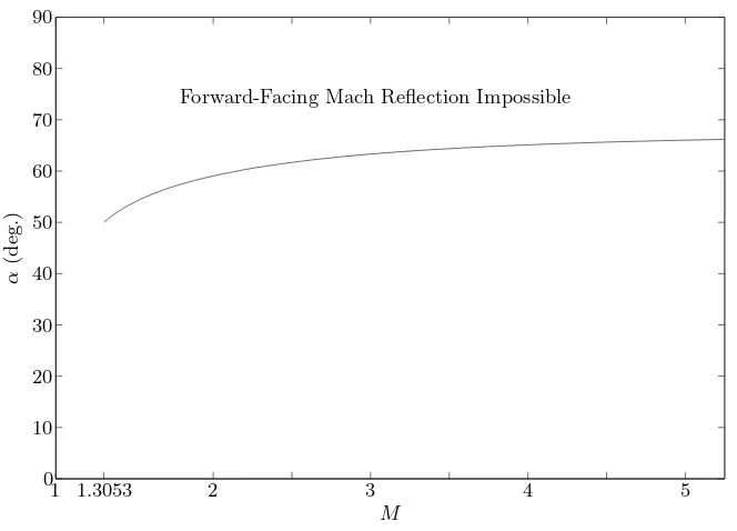
2.3.7 Sonic Forward-Facing Reflected Shock Condition . . . 31
7 Experimental Hysteresis 125
8 Experimental Transition 131
8.1 Energy Deposition Location . . . 134
8.2 Tunnel Disturbances . . . 134
9 Experimental Mach Stem Heights 139
9.1 Experimental Mach Stem Growth . . . 140
10 Conclusions and Future Work 143
A Mach Reflection Domain 147
B Alternative Plots 152
C Mach 4 Nozzle Design 156
D Double Wedge Model 174
D.1 Adjustable Wedge Model . . . 174
D.2 Fixed Wedge Model . . . 183
List of Figures
1.1 Pseudosteady regular reflection and Mach reflection. . . 2
1.2 Steady regular reflection and Mach reflection. . . 2
1.3 Steady von Neumann reflection. . . 3
2.1 Basic flow parameters for a wedge with an attached shock. . . 10
2.2 Regular reflection with supersonic downstream flow. . . 11
2.3 Regular reflection with subsonic downstream flow. . . 12
2.4 Mach reflection. . . 13
2.5 Mach reflection with subsonic downstream flow. . . 14
2.6 Mach reflection with a forward-facing reflected shock. . . 15
2.7 Inverted Mach reflection. . . 16
2.8 Von Neumann reflection. . . 16
2.9 Flow over a zero-degree wedge producing a Mach wave. . . 17
2.10 Shock reflection domain, forγ = 1.4, considering only the Mach wave condition. 18 2.11 Shock reflection domain, for γ = 1.4 considering only the sonic incident shock condition. . . 19
2.12 Flow over a wedge producing an incident and reflected shock. . . 19
2.13 Example of the detachment condition for M = 4 and γ = 1.4. . . 20
2.14 Shock reflection domain, for γ = 1.4 considering only the detachment condition. 22 2.15 Flow over a wedge producing a triple point at the von Neumann condition. . 23
2.16 Example of the von Neumann condition for M = 4 and γ = 1.4. . . 23
2.17 Shock reflection domain, for γ = 1.4 considering only the von Neumann con-dition. . . 27
the wedge and the two vertical supports. . . 123
7.1 Demonstration of the hysteresis phenomenon in the Ludwieg tube. The initial
wedge angles are set so that only regular reflection is possible. . . 126
7.2 Demonstration of the hysteresis phenomenon in the Ludwieg tube. The
condi-tions are within the dual solution domain, just below the point where transition
to Mach reflection will occur due to tunnel disturbances. . . 126
7.3 Demonstration of the hysteresis phenomenon in the Ludwieg tube. Transition
to Mach reflection is just beginning to occur due to tunnel disturbances. . . . 127
7.4 Demonstration of the hysteresis phenomenon in the Ludwieg tube. The upper
wedge angle is relatively large, and a large Mach stem exists. . . 127
7.5 Demonstration of the hysteresis phenomenon in the Ludwieg tube. The upper
wedge angle is relatively large, and a large Mach stem exists. . . 128
7.6 Demonstration of the hysteresis phenomenon in the Ludwieg tube. Return to
regular reflection as the von Neumann condition is approached. . . 129
8.1 Initial shock configuration below the von Neumann condition. Only regular
reflection is possible. . . 132
8.2 Shock configuration before laser energy is deposited onto the lower wedge.
Both regular reflection and Mach reflection are possible. . . 132
8.3 Blast wave resulting from the deposition of energy on the lower wedge using
a laser. . . 133
8.4 The leading shock is disturbed in the region of the reflection due to the laser
energy, which was previously deposited. Transition to Mach reflection will
immediately follow. . . 133
8.5 Energy deposition points on the lower wedge. . . 135
8.6 Effect of wedge rotation speed on tripping due to natural tunnel disturbances. 136
8.7 Tunnel disturbances, such as dust, are capable of tripping the flow from regular
theoret-D.4 Motor mount (part 9) drawing. . . 178
D.5 Rocket (part 10) drawing. . . 179
D.6 Moving wedge (part 11) drawing. . . 180
D.7 Rocker housing (part 16) drawing. . . 181
D.8 Rocker housing lid (part 17) drawing. . . 182
D.9 Fixed wedge model assembly drawing of the various primary components and their relationships to each other. . . 184
D.10 Fixed wedge (part 1) drawing. . . 185
D.11 Vertical support (part 2) drawing. . . 186
List of Tables
8.1 Summary of transition for various energy deposition locations. . . 134
9.1 Mach stem heights measured at various upper wedge angles. . . 139
C.1 Mach 4 nozzle contour (in inches) by J. J. Korte. . . 156
C.2 Primary components of the Mach 4 nozzle. . . 164
D.1 Primary components of the adjustable wedge model. . . 174
Chapter 1
Introduction
When a shock wave propagates over a solid wedge, the flow generated by the shock impinges
on the wedge thus generating a second reflected shock, which ensures that the velocity of
the flow is parallel to the wedge surface. Viewed in the frame of the reflection point, this
flow is locally steady, and the configuration is referred to as a pseudosteady flow. When
the angle between the wedge and the primary shock is sufficiently large, a single reflected
shock is not able to turn the flow to a direction parallel to the wall and transition to Mach
reflection occurs. These are illustrated in Figure 1.1
Much of the research in the field of Mach reflection has been done in this pseudosteady
configuration. The concern of this thesis, however is the transition between regular and
Mach reflection in steady flow. If a wedge is placed into a steady supersonic flow in such
a way that its oblique attached shock impinges on a flat wall parallel to the free stream,
the shock turns the flow toward the wall and a reflected shock is required to turn the flow
back to a direction parallel to the wall. When the shock angle exceeds a certain value, the
deflection achievable by a single reflected shock is insufficient to turn the flow back to a
direction parallel to the wall and transition to Mach reflection is observed. Both regular
reflection and Mach reflection in steady flow are illustrated in Figure 1.2.
The fundamental question regarding regular reflection and Mach reflection, is at which
flow conditions they occur.
Most steady flow studies of shock reflection have considered a wedge placed above a
planar surface. In experiments, the planar surface is most often replaced by a plane of
symmetry in order to remove boundary layer effects. In his 1943 report, von Neumann [1]
also considered this problem. He did so by first considering regular reflection, where the
(a) (b)
Figure 1.1: Pseudosteady regular reflection (a) and Mach reflection (b). The primary shock is traveling from left to right over the wedge.
(a) (b)
Figure 1.3: Steady von Neumann reflection. The free-stream flow is from left to right.
reflected shock is to turn the flow from behind the incident shock back to its initial angle.
However, he considers the fact that the reflected shock has a maximum turning angle, and
therefore a reflection directly off the planer surface (regular reflection) may not always
be possible. Based on this maximum turning angle, he defines what he calls the extreme
condition, which would later come to be known as the detachment condition. Simply put,
the detachment condition is the largest incident shock angle for which the oblique reflected
shock can turn the flow back to its original angle.
Von Neumann [1] in his analysis of Mach reflection considers the pseudosteady case.
He defines Mach reflection as the configuration in which the incident shock does not reflect
off the planar surface, but rather reflects from a triple point above the planar surface. In
addition to the reflected shock from this triple point there is an additional shock, the Mach
stem, which lies between the triple point and the planar surface. Also, a slipline originates
from this triple point because of the different flow conditions behind the reflected shock and
behind the Mach stem; even though the pressures behind both are the same.
In addition, von Neumann [1] postulates the possibility for what he calls quasi-stationary
Mach reflection, which in the case of steady flow is simply Mach reflection. The condition
for quasi-stationary Mach reflection is that the pressure behind the reflected shock is equal
to the pressure obtained behind a stationary normal shock. This condition would later be
renamed the von Neumann condition. For low Mach numbers von Neumann calculated
that Mach reflection was not possible, although something resembling Mach reflection
ex-isted in experiments. He called this type of reflection extraordinary Mach reflection, which
would later be renamed von Neumann reflection. Von Neumann reflection is illustrated in
Figure 1.3.
The conclusion of von Neumann [1] is that in the parameter range where Mach reflection
inside the dual-solution domain. For the case of a dense particle, the importance of
the impact shock, created when the particle impacts one of the wedges, is observed.
• Experiments show that using the newly constructed Mach 4.0 nozzle and the
exist-ing Ludwieg tube, hysteresis between regular reflection and Mach reflection can be
observed. Regular reflection was maintained approximately halfway into the
dual-solution domain. It is experimentally shown that the faster the shock configuration
enters the dual-solution domain the further into the dual-solution domain regular
reflection can be maintained.
• Experiments show that depositing energy onto one of the wedges can cause transition
from regular reflection to Mach reflection. The importance of the deposition location
is observed and is qualitatively consistent with the numerical and theoretical work of
this thesis.
• Both the steady-state Mach stem height and Mach stem growth rate were measured
experimentally. Excellent agreement between the Mach stem height theory, developed
in the thesis, and experimental measurements is seen. The time to reach the
steady-state Mach stem height agrees well with the theory developed in this thesis, although
M >1
M >1
M >1
P P∞
θ0(deg.) 1
(a) (b)
Figure 2.2: Regular reflection with supersonic downstream flow. Part (a) shows an example of regular reflection with supersonic flow downstream of the reflected shock. For simplicity the expansion wave originating from the downstream corner of the wedge is not shown. Part (b) shows an example shock polar diagram demonstrating regular reflection.
2.2
Possible Shock Reflections
There are several possible shock reflections. These are regular reflection with supersonic
downstream flow (RR), regular reflection with subsonic downstream flow (RRs), Mach
re-flection with supersonic flow downstream of the reflected shock (MR), Mach rere-flection with
subsonic flow downstream of the reflected shock (MRs), Mach reflection with a forward
facing reflected shock (MRf), inverted Mach reflection (IMR), and von Neumann reflection
(vNR).
2.2.1 Regular Reflection
The simplest configuration possible is regular reflection with supersonic flow downstream of
the reflected shock. An example of regular reflection is shown in Figure 2.2(a). In this case,
the reflected shock turns the flow by the exact same amount as the incoming shock, i.e., the
reflected shock turns the flow by the wedge angle so that the flow is again parallel to the
free-stream flow. The reflected shock, in this case, is sufficiently weak that the flow behind
it remains supersonic. Figure 2.2(b) shows an example shock polar with regular reflection.
The point where the reflected shock polar intersects the zero deflection line is denoted with
1 1
∞
M∞
Figure 2.9: Flow over a zero-degree wedge producing a Mach wave. The flow in region 1 is therefore identical to the free-stream flow.
2.3
Domain Boundaries
2.3.1 Mach Wave Condition
For any given free-stream Mach number,M∞, a minimum shock angle exists. This angle is
the Mach wave angle, αMW, and is given simply by
αMW=αμ(M∞). (2.7)
This defines the lower boundary of the Mach reflection domain, since no incident shock
can exist with a shock angle less than αMW. A Mach wave produces a zero-flow deflection
angle. A representative Mach wave is shown in Figure 2.9. An example of the shock
reflection domain considering only the Mach reflection condition is shown in Figure 2.10.
2.3.2 Sonic Incident Shock Condition
If the incident shock is strong (i.e., if the flow behind the incident shock is subsonic), a
reflected shock is not possible; therefore, no shock reflection can occur. This sets the upper
boundary for the reflection domain since no incident shock with a higher angle can produce
a shock reflection. This boundary is defined by the flow behind the incident shock being
sonic. Specifically, the relation for the leading shock angle at this condition, αSIS, is given
by
1 2 3 4 5 0
10 20 30 40 50 60 70 80 90
α
(deg
.)
M
Shock Reflection Impossible
Figure 2.11: Shock reflection domain, forγ = 1.4 considering only the sonic incident shock condition.
1
2
∞
αD (θ 1)D
-401 -30 -20 -10 0 10 20 αD30 40 50 60 10
100
P P∞
θ (deg.)
Figure 2.13: Example of the detachment condition for M = 4 and γ = 1.4. Note that the maximum deflection of the reflected shock corresponds to θ = 0. The ∗ denotes the sonic points of the shock loci.
the same. The Mach number behind the leading oblique shock at this condition is
(M1)D =M(M∞, γ, αD). (2.10)
Therefore the following must be satisfied,
θ(M∞, γ, αD) =θ
(M1)D, γ, αθmax((M1)D, γ)
. (2.11)
Solving Equation 2.11 forαD produces a fifth-order polynomial in sin2αD,
1
2 3
∞
αvN
Figure 2.15: Flow over a wedge producing a triple point. At the von Neumann condition the Mach stem is normal to the free-stream flow and therefore the flow behind it is parallel to the bottom surface. In addition, both the pressure and flow angle behind that reflected shock match that of the normal Mach stem.
-401 -30 -20 -10 0 10 αvN 30 40 50 60
10 100
P P∞
θ (deg.)
1 2 3
∞
αNRS
Figure 2.21: Flow over a wedge producing a reflected shock that is perpendicular to the flow behind the incident shock.
-151 -10 -5 0 5 αNRS 15 20 2
3
P P∞
θ (deg.)
-151 -10 -5 0 αSFRS 10 15 2
P P∞
θ (deg.)
Figure 2.25: Example of the sonic forward-facing reflected shock condition for M = 1.45 and γ = 1.4. Note that the intersection of the reflected and incident shock polars occurs when the reflected shock is forward facing and at its sonic point. The∗ denotes the sonic point of the shock loci.
reflected shock condition can be written as
ξ(M∞, γ,(αs)SFRS) =ξ(M∞, γ, αSFRS)ξ((M1)SFRS, γ,(α1)SFRS), (2.59)
θ(M∞, γ,(αs)SFRS) =θ(M∞, γ, αSFRS) +θ((M1)SFRS, γ,(α1)SFRS), (2.60)
where (αs)SFRS is the angle of the Mach stem with respect to the incoming flow, and
(α1)SFRS =α∗((M1)SFRS, γ), (2.61)
(M1)SFRS =M(M∞, γ, αSFRS). (2.62)
Note that Equations 2.59 through 2.62 are identical to Equations 2.46 through 2.49 except
Chapter 3
Mach Stem Height Prediction
Consider the reflection of a shock, generated by a wedge in steady supersonic flow, from a
wall (single wedge configuration) or from a plane of symmetry (double wedge configuration).
For a sufficiently high free-stream Mach number, there exists a range of wedge angles (the
dual-solution domain) in which both regular and Mach reflection are possible. To date there
is no accurate method of predicting the height of a Mach stem in steady flow. Predictions of
Mach stem height can be important in the design of supersonic inlets if the inlet is expected
to experience Mach reflection. An accurate prediction of the Mach stem height may also be
useful in understanding the behavior of the shock reflection in the dual-solution domain.
Azevedo [7, 18] (see also Ben-Dor [19]) developed a theory based on the location of
the sonic throat formed by the initially converging flow behind the Mach stem. However,
his prediction consistently underestimated the actual Mach stem height. The aims of the
present work are to relax some of the assumptions made by Azevedo in order to obtain more
accurate predictions of Mach stem height, and to analyze the rate of growth of a Mach stem
starting from a regular reflection in the dual solution domain. Work by Li and Ben-Dor [20]
corrects some of the flaws in the theory of Azevedo, but gives very similar approximations
of Mach stem height, which differ significantly from the experimental work of Hornung and
Robinson [6]. The works by Li et al [21] and Schotz et al. [22] consider downstream influences
on Mach stem height; however, the experimental work of Chpoun and Leclerc [23] shows
that the Mach stem height does not vary with downstream conditions. This is as expected,
since the flow in the expansion region and downstream of the sonic throat is supersonic and
therefore these influences cannot affect Mach stem height. There is therefore no need in the
current work to consider the flow downstream of the expansion wave corresponding to the
3.1
Problem Setup
The problem setup is shown graphically in Figure 3.1. We can either consider two opposing
wedges, or for inviscid flow, a wedge above a flat plate. The wedge, with a length w, is
declined at an angle θ1 with respect to the free-stream flow and produces a shock at an
angle α. The height of the triple point above the surface is the Mach stem height, denoted
s. In the case of two symmetric wedges, sis half the total Mach stem height. At the triple
point a slipline is created, which is initially declined at an angleδ with respect to the surface
or plane of symmetry. The reflected shock from the triple point is inclined at an angle φ
with respect to the surface.
In general the Mach stem height, s, is a function of the Mach number,M, the ratio of
specific heats, γ, the spacing between the wedge and the flat surface, g, the angle of the
wedge,θ1, and the wedge length,w. That is to say
s=f(M, γ, g, θ1, w), (3.1)
wheref is an unknown function. Nondimensionalizing this relationship we find that
s+=f+M, γ, g+, θ1, (3.2)
wheref+is the nondimensional version off,s+ = ws, andg+= wg. Normalizing lengths by
w is a good choice, since, in experiments,w will almost always be a fixed length and not a
function of the wedge angleθ1.
3.2
Mass and Momentum Balance
Azevedo [7] considers a problem setup as shown in Figure 3.1 subject to several
assump-tions. First, he assumes that the sonic throat occurs where the leading characteristic of
the expansion fan intersects the slipline. Second, he assumes that the region between the
slipline and the symmetry plane, and between the Mach stem and the sonic throat is an
isentropically converging ideal gas flow with a straight streamlineT H. To analyze the flow
Azevedo applies conservation of mass and momentum.
flow entering between the wedge tip,O, and the symmetry plane. This mass flow can then
be equated to the mass flow through EF, F H, and s . Equating these two mass fluxes
produces the following equation:
ρ∞u∞(g+wsinθ1) =ρ1u1sinμ1EF +ρ2u2sinμ2F H +ρ u s , (3.3)
whereμ1 and μ2 are the Mach angles and are given by
μ1 = sin−1 1
M1, (3.4)
μ2 = sin−1 1
M2. (3.5)
Next, he considers the conservation of momentum in the free-stream flow direction.
Equat-ing the pressure and momentum flux between the wedge tip and the solid surface with the
pressure and the momentum flux throughEF,F H, ands produces
P∞(g+wsinθ1)−P1wsinθ1+ sin (μ1+θ1)EF−P2sin (μ2+δ)F H −P s
=ρ1u21sinμ1cosθ1EF +ρ2u22sinμ2cosδ F H+ρ u2s −ρ∞u2∞(g+wsinθ1). (3.6)
Similarly, for conservation of momentum perpendicular to the free-stream flow direction, he
finds that
P∞(xs+wcosθ1) +P3x −P1wcosθ1+ cos (μ1+θ1)EF−P2cos (μ2+δ)F H
=−ρ1u21sinμ1sinθ1EF −ρ2u22sinμ2sinδ F H. (3.7)
Azevedo takesP3to be the average pressure in Region 3, which is the average of the pressure
at the sonic throat and the pressure right behind the Mach stem. The numerical result is
almost identical if we takeP3 to be the integrated pressure using the area ratio relationship.
Equations 3.3, 3.6 and 3.7 can be written in nondimensional form with the superscript+
refering to nondimensional quantities. Specifically, density is normalized by the free-stream
density, ρ∞, velocities are normalized by the free-stream velocity, u∞, pressures are
important to note that there is no simple way of matching the pressure across the slipline.
Since the pressure is not correct a solution that tries to conserve momentum is also incorrect
and produces an inconsistent geometry. Therefore, it may be useful to fix the geometry and
continue to allow the pressure across the slipline to be mismatched.
3.3
Geometric Solution
In Azevedo’s solution the most restrictive assumption is that the sonic throat occurs at the
leading characteristic of the expansion fan. Also, Azevedo does not force the geometry to
be self-consistent, specifically, the condition that the slipline, T H intersects the expansion
wave, F H, and the sonic throat at a point is not imposed. To solve the latter problem
we can write five equations that fix the geometry, assuming that all shocks and sliplines
are straight. It is important to not that these equations implicitly satisfy the mass and
momentum equations because the shock-jump conditions, which are used to generate the
geometry, satisfy the mass and momentum equations. These equations are
sinα OT +s=g+wsinθ1, (3.69)
s + sin (δ+μ2)F H + sin (μ1+θ1)EF =g, (3.70)
cosα OT+ cosδ T H−cos (δ+μ2)F H−cos (μ1+θ1)EF =wcosθ1, (3.71)
cosα OT+ cosφ T F −cos (μ1+θ1)EF =wcosθ1, (3.72)
sinα OT −sinφ T F −sin (μ1+θ1)EF =wsinθ1. (3.73)
Given the area ratio betweensand s , we can write cosδ T H as
O
E
F
H s
g w
T
s
θ1
α
δ
φ
∞
1
3
a
Figure 3.3: Flow setup, allowing for a sonic throat downstream of the leading characteristic, used to predict the Mach stem height.
3.4
Generalized Geometric Solution
The problem still remains that all of these solutions assume that the sonic throat of the
flow behind the Mach stem occurs at the leading characteristic of the expansion fan. To
eliminate this problem, we will allow the sonic throat to occur further downstream. This
generalized setup is shown in Figure 3.3. The geometrical considerations are the same as
those leading to Equation 3.80, withF andHreplaced byF andH, respectively. Also,μ1
and μ2 refer to the Mach angle along the characteristic corresponding to the sonic throat,
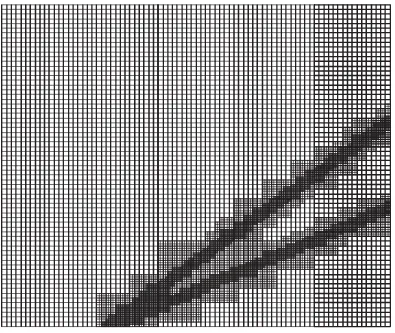
Figure 3.4: Representative mesh refinement for the calculation of the Mach stem height using Amrita.
g
δ
φ w
θ1
∞
1
α
Utp
a 3
Figure 3.7: Flow setup, allowing for a moving triple point, used to calculate the Mach stem height growth.
3.7
Moving Triple Point Analysis
The triple point analysis presented earlier assumed a stationary Mach stem. We will now
consider the case where the Mach stem moves with an upstream velocity, UMs, subject to
a quasi-steady flow assumption. This may occur in a steady free stream, e.g., if transition
to Mach reflection is initiated by some disturbance when the flow is initially in the
dual-solution region. The rate at which the Mach stem moves upstream, UMs, is related to the
speed at which the triple point travels up along the lead shock,Utp, by
Utp= UMs
cosα. (3.86)
Figure 3.7 shows the flow setup when the triple point is moving.
To perform the triple-point analysis we must examine the flow both in the lab-fixed
reference frame and in the frame of the triple point. Quantities calculated in the reference
1 100
0 10
10 20 30 40 Stationary Shock Polar
Moving Triple Point
θ(deg.)
P P∞
Figure 3.9: Shock polar illustrating the effects of a moving Mach stem. In the case where the Mach stem is moving upstream the pressure ratio is higher than the stationary-case value, and vice-versa. Each point on the moving triple point curve represents the pressure and deflection angle for a given Mtp. M∞=4, γ=1.4,θw=24◦.
be moving downstream so fast that the relative flow into the reflected shock is subsonic.
This means that the perpendicular component of the flow into the reflected shock must be
supersonic. As the flow speed into the reflected shock decreases, the pressure rise across
the reflected shock also decreases, and we would expect the pressure and the flow deflection
to be similar to that of the leading shock alone. In other words, as the triple point moves
downstream, the jump across the reflected shock becomes weaker and the flow deflection
across the reflected shock decreases. This is indeed seen in Figure 3.9, where the moving
triple-point line terminates near the incident shock point.
3.8
Mach Stem Height Variation
As the Mach stem grows, it also slows down. Thus, for a given Mach stem speed a
corre-sponding Mach stem height exists. Using Equation 3.81 and substituting the modified flow
parameters, as found in Section 3.7, it is possible to calculate the Mach stem height at a
the steady-state height, in particular, the speed of the Mach stem during the Mach stem
growth phase.
To understand the growth phase of the Mach stem, let us consider a very small Mach
stem, as is shown in Figure 3.10. If the Mach stem were stationary, the slipline originating
from the triple point would have a finite angle and therefore reach the wall before the
leading characteristic. Since it is not physically possible for the slipline to intersect the wall
we know that this solution can not be correct, and therefore the Mach stem must move in
order to produce a different slipline angle. Specifically, we need the slipline angle to be at a
small enough angle such that it reaches the first characteristic. We therefore now know that
the triple point must move in a way as to decrease the slipline angle. Let us now consider a
slipline angle sufficiently small that it intersects the first characteristic just above the wall.
In this case, the area ratio between the Mach stem and the intersection of the slipline with
the first characteristic would be very large.
From Figure 3.9, we see that the deflection angle is decreased if the shock is moving
upstream. Additionally, the flow Mach number behind the Mach stem will decrease if the
Mach stem moves upstream, which produces a large area ratio. Based on this we can
hypothesize that for small Mach stems, the Mach stem must travel upstream. Based simply
on geometry, a Mach stem traveling upstream also increases in height.
The moving Mach stem changes the slipline angle, δ, the reflected shock angle, φ, the
Mach angle in region 2, and the area ratio between the Mach stem and the sonic throat,
Ar. Assuming quasi-steady flow, that is to say, the speed at which the triple point grows
g w
θ1
α
∞
1
−0.25 0 0.25 0.5
0 0.2 0.4 0.6
s/w
M
tp
Figure 3.11: Mach stem velocity as a function of Mach stem height based on Equation 3.80. Positive Mtp indicates upstream speed. Calculated for M∞=4, g/w=0.4, γ=1.4, and
θ1=25◦.
height growth for a wedge angle ofθ1=23◦.
In Figure 3.13 we see that the predicted Mach stem height is about 60% greater than
in the numerical computation. This figure represents what is a relatively extreme case.
Specifically, the numerically calculated Mach stem height,s/w, is slightly under 0.2, whereas
most theoretical predictions of Mach stem height, including those presented in this thesis,
only appear to be valid for Mach stem heights below about 0.1. Experimental results
presented later in this thesis show that for large Mach stems, the theory developed in this
thesis significantly over predicts the Mach stem height. We see in Figure 3.14, that there is a
significant difference between the shape of the slipline originating from the triple point and
the slipline used in the theoretical estimate. Specifically, the computed slipline gradually
approaches 0◦ thereby giving it a lower average angle. This lower average angle causes a
decrease in the Mach stem height. For the cases considered, the theory appears to locate
0 0.02
0.04 0.06 0.08
0 2 4 6 8
c∞t/w
s/
w
Numerical Theoretical
Figure 3.12: Theoretical and numerical results for the height of the Mach stem as a function of time as it grows from an initial regular reflection condition. Calculated for M∞ = 4, g/w= 0.3907, γ = 1.4, andθ1= 23◦.
0 0.1 0.2 0.3
0 2 4 6 8
c∞t/w
s/
w
Numerical Theoretical
Figure 3.14: A quasi-schlieren image showing a comparison between the theoretical shock structure and an Euler computation. The image shows that the shape of the slipline in the computation is significantly different from what is assumed in the theory. This difference between computation and theory most likely accounts for most of the error between the two. The theoretical lines are shown as dotted lines. Calculated forM∞ = 4, g/w = 0.42, γ = 1.4, andθ1= 25◦.
3.9
Three-Dimensional Mach Stem Growth
Consider a three-dimensional flow with a regular reflection in the dual-solution domain.
When a Mach stem is first formed, it is both small in height and in width in the spanwise
direction. As it grows it both increases in height and expands outward in the spanwise
direction. This opening is referred to as a mouth because of its shape [11]. The spanwise
region where the transition from a Mach stem to a regular reflection occurs is characterized
by a 5-point theory. This point exists at the intersection of five shocks, those being the
incoming shock, the regularly reflected shock, the Mach stem, the Mach stem reflected shock,
and a fifth shock dividing the downstream flow region between the regular reflection and
the Mach reflection. Farther away from this point, we can expect the behavior of the Mach
stem to follow that of the two-dimensional theory in the appropriate frame of reference. We
can therefore conclude that the expansion rate of the Mach stem in the spanwise direction
is determined by a complex system of five shocks; whereas, the overall change in height of
the Mach stem is governed by the two-dimensional theory presented in Section 3.8. Using
the two-dimensional theory for the height and setting the spanwise expansion of the Mach
stem to a constant, produces the evolution of a Mach stem that is seen in Figure 3.15. This
0.01 0.02 0.03 0.04 0.05 0.06
-10 -5 0
0 5 10
x wMx
s/
w
Figure 3.16: Growth of a Mach stem considering a Mach stem with an initial finite width,
s, and spanwise width of Mach stem,x, which is propagating outward at a Mach number,
Mx. Curves for flow times (a∞t/w) between 1 and 10, in increments of 1, with the lower
curves corresponding to lower times. Calculated for M∞ = 3, g/w = 0.4516, w = 150, γ = 1.4, andθ1= 21◦.
it will depend only on the local flow conditions around the five shock solutions; therefore,
x
c∞t =h(M∞, γ, θw), (3.109)
which gives a constant spanwise expansion speed for any given flow parameters. The use
of the two-dimensional theory from Section 3.7 and the best-fit spanwise growth rate yields
very good agreement to computations. Figures 3.17 through 3.19 show the progression of
0.01 0.02 0.03 0.04 0.05
-1.50 -1 -0.5 0 0.5 1 1.5
x wMx
s/
w
Numerical Theoretical
Figure 3.19: Numerical and theoretical growth of Mach stem height, s, and growth in the spanwise direction, x, at c∞t/w=0.79. The Mach stem is propagating outward at a Mach number, Mx = 0.5916. Calculated for M∞ = 3, g/w = 0.4516, w = 150, γ = 1.4, and
Chapter 4
Dense Gas Disturbances
It has been observed by Sudani et al. [11] that water vapor can cause transition to occur
closer to the von Neumann condition than it does otherwise. The studies by Sudani et al.
did not fully account for the mechanism by which water vapor causes transition from regular
reflection to Mach reflection. This section will present two-dimensional computations where
water vapor is modeled as a dense and cold region of gas. Calculations where the impact of
the dense gas on the wedge is modeled as an energy deposition are also presented. In the
case of energy being deposited on the surface of the wedge, a minimum required energy for
transition is given. In addition, several three-dimensional calculations were performed. In
all computations presented here, the free-stream pressure and density are set to unity.
4.1
High Density Gas Region
Numerical studies using high-density gas regions were conducted in both two dimensions
and three dimensions. The results of these studies are presented in this section.
The first set of numerical studies model the disturbance as a small, cold, and dense
region of gas. Initially, the gas has the same pressure and velocity as the free stream.
All two-dimensional computations were performed using Amrita [24] with the assistance of
James Quirk. The details of the Amrita system are discussed in Section 3.5. In all the
cases, the free-stream Mach number was set to 4, and the ratio of specific heats was set to
1.4. The computational domain was 300 cells wide and 240 cells high. Each cell could be
refined to either 9 cells or 81 cells depending on the local density gradient. The geometry
g G
d
w
θ1
∞
1
α
Reflected Bow Shock
Disturbed Bow Shock
Recompression Shock
Reflected Bow Shock
Impact Shock
Reflected Bow Shock
Impact Shock
Figure 4.7: Quasi-schlieren image showing the reflected bow shock and impact shock from an area of gas with an initial radius of 1 cell and an initial density of 1500 times the free-stream density after they have reached the leading oblique shock. The dense gas originated 75 cells above the centerline, and the wedge angle is 25◦.
Figure 4.7, both the reflected bow shock and the impact shock reach the leading shock.
As the impact shock travels downstream it will pass over the reflection point, and locally
increase the shock angle. This is seen in Figure 4.8.
If the disturbance is strong enough, a Mach stem will form. The first sign of a Mach
stem is shown in Figure 4.9.
Once the Mach stem is formed a communication link between the expansion wave and
the Mach stem is created. This communication tells the Mach stem how large it should
be, and it will continue to grow until it reaches its steady state height. An example of this
Reflected Bow Shock
Impact Shock
g G
d
l1
l2
Rs(t)
w
θ1
∞
1
α
d
E0
×
10
4
0 4 8 12
50 60 70 80
θ1= 22◦
θ1= 25.5◦
Figure 4.21: A lower bound on the energy, E0, required for the blast wave to reach the
point of reflection. If the energy added is less than this minimum energy, transition from regular to Mach reflection is impossible. Computations done for M = 4, ρ∞ = 1, ν = 2, γ = 1.4, andG= 120. The wedge angle, θ1, varies between 22◦ and 25.5◦ in increments of
d
E0
×
10
6
0 2 4 6
50 60 70 80
θ1= 22◦
θ1= 25.5◦
Figure 4.22: A lower bound on the energy, E0, required for the blast wave to reach the
point of reflection. If the energy added is less than this minimum energy, transition from regular to Mach reflection is impossible. Computations done for M = 4, ρ∞ = 1, ν = 3, γ = 1.4, andG= 120. The wedge angle, θ1, varies between 22◦ and 25.5◦ in increments of
Yesy
d
E0
×
10
4
0 1 2 3
60 70 80
Theoretical Numerical Transition
Figure 4.23: Energy, E0, required for transition from regular to Mach reflection to occur.
Chapter 5
Asymmetric Oblique Shocks
The theory for the reflection of two shocks at different angles with respect to the flow can
be developed in much the same way as was done in Chapter 2. A generalized setup allowing
for different oblique shock angles in presented in Figure 5.1.
For the purposes of this section, we will limit ourselves to higher Mach numbers, and
consider only Mach reflection and regular reflection, allowing for subsonic flow downstream
of the reflected shock. First we will consider the detachment condition. For shock angles
greater than this condition, regular reflection can not exist. In Section 2.3.3, we said the
flow angle behind the reflected shock must be equal to that of the incoming flow; however,
when there are two incident shocks of different angles this is no longer true. The flow
directions after the reflected shocks must be the same; however, they do not need to be
parallel to the free-stream flow. An example shock polar at the detachment condition is
shown in Figure 5.2. The detachment condition for asymmetric wedges is defined simply
as the point at which the two reflected shock polars intersect once and are tangent at the
intersection. This condition can also be thought of as the point where any further separation
of the reflected shock polars would result in no intersection of the two polars. A plot of the
detachment condition for various Mach number is shown in Figure 5.3. Figure B.1 is the
detachment condition plotted with shock angles rather than deflection angles.
Similarly, an example shock polar at the von Neumann condition is shown in Figure 5.4.
This condition occurs when both reflected shock polars and the incident shock polar intersect
one another at a single point. A plot of this condition for various Mach numbers is shown
in Figure 5.5. Figure B.2 is a similar plot of the von Neumann condition, but plots the
shock angles instead of the deflection angles.
Fig-2g w
θupper
αupper
θlower
αlower
αlower(deg.)
αupp
er
(deg
.)
15 25 35 45 55 65
20 30 40 50 60 Von Neumann Condition Equivalence Curves
Figure 5.7: Dashed lines represent equivalence curves, with the * representing the symmetric case. Cases that are only slightly different than the symmetric case can be related to the symmetric case that lies on their equivalence curves.
angle space, from the von Neumann condition can be used. These equivalence curves, i.e.,
Chapter 6
Experimental Setup
Several experiments were conducted using the Ludwieg Tube at the Graduate Aeronatuical
Laboratories of the California Institute of Technology (GALCIT). The details of the facility
and the specific test setup will be discussed in this chapter.
6.1
Ludwieg Tube
A Mach 4 nozzle was designed, constructed and taken into operation for the existing Ludwieg
tube at GALCIT. The Ludwieg tube consists of a 17 m long 300 mm inner diameter tube,
a transition piece to allow for the upstream insertion of particles, an axisymetric nozzle, a
diaphragm station (located either just upstream of the throat or downstream of the test
section) and a dump tank; see Figure 6.1.
Before a run, the tube is filled with the test gas at a pressure of up to 700 kPa and
the dump tank is evacuated. To start the run, the diaphragm is ruptured, thus causing an
expansion wave to propagate through the nozzle and into the tube. When the diaphragm is
in the downstream position, the diaphragm is ruptured in a controlled way using a cutting
device. In the future upstream position, the diaphragm is ruptured by creating a sufficient
pressure difference across the diaphragm, since any cutting device upstream of the nozzle
would disrupt the flow. During the time it takes for the expansion wave to travel to the
end of the tube and for the reflected wave to return to the nozzle, the reservoir conditions
for the nozzle flow are almost perfectly uniform, thus giving a constant condition test time
of 80 to 100 ms.
A Mach number of 4 was chosen because it is necessary to operate at a Mach number
Figure 6.1: Overview drawing of the Ludwieg tube laboratory. The dump tank is shown on the right, the expansion tube on the left, and the test section in between.
avoid having to heat the gas in the tube, it is necessary to operate at a Mach number no
higher than 4, to avoid condensation of the test gas in the nozzle expansion.
At this Mach number it was better to make the nozzle axisymmetric rather than
rect-angular. In part, this is to eliminate the unavoidable secondary flow in the corners, and
the complications of a circular to rectangular transition piece. Since the test rhombus is
very slender at Mach 4, a considerable portion of the test rhombus lies downstream of the
nozzle exit, so that a useful portion of the test section can be fitted with flat windows set
back from the nozzle edge, so that no reentrant corner is visible to the flow.
The contours for the Mach 4.0 nozzle, shown in Figure 6.4 and listed in Table C.1, and
the original Mach 2.3 nozzle were designed by J. J. Korte of NASA Langley Research Center.
Korte [30, 31, 32] uses an efficient code to solve the parabolized Navier-Stokes equations
and couples this with a least-squares optimization procedure. The objective function of the
least-squares routine consists of the Mach number distribution along the centerline and the
exit profile of both the Mach number and flow angle. By doing this, the nozzle contour is
designed to compensate for viscous effects. Detailed drawings of the Mach 4.0 nozzle are
shown in Appendix C. The Mach 2.3 nozzle has been calibrated by using the weak Mach
wave technique. Weak waves are generated by thin adhesive strips taped to the walls. These
are visualized using the schlieren technique, thus giving a pattern of lines that correspond
very closely to the characteristics in the flow, see Figure 6.2. Measurement of the angles
at the intersection of these lines gives the Mach number and flow angle distribution in the
1 1.5 2 2.5
0 10 20 30 40 50 60 70 80 90 100
x(cm)
M
Shock Expansion Computation
x(cm)
r
(cm)
-20 0 20
0 30 60 90 120
Figure 6.4: Mach 4.0 nozzle contour designed by J. J. Korte of NASA Langley Research Center.
when the diaphragm separates the high pressure gas in the tube and nozzle from the low
pressure region in the dump tank. At t = 4 ms the shock generated by the diaphragm
rupture has traveled downstream into the dump tank and an expansion wave propagates
upstream through the nozzle. At t= 8 ms the expansion wave has partially reflected from
the nozzle and formed a reflected shock, this shock is seen just downstream of the throat.
Att= 12 ms andt= 16 ms the reflected shock continues to travel downstream through the
nozzle. It is important to note that the reflected shock is moving against the nozzle flow
and therefore travels slowly in the lab-fixed frame. At t = 20 ms the reflected shock has
traveled downstream past the first expansion characteristic from the end of the nozzle, and
steady flow in the test section is established. A 20 ms startup time is quite acceptable and
is almost identical to the startup time with the previous Mach 2.3 nozzle.
Early experiments showed that the flow, using the downstream diaphragm, did not
properly start. An image taken halfway through the test time is shown in Figure 6.6. The
maximum steady flow time achieved with this configuration was no more than 20 ms.
Amrita simulations were conducted to understand the problem, in particular, the
t= 0 ms
t= 4 ms
t= 8 ms
t= 12 ms
t= 16 ms
t= 20 ms
Figure 6.6: Experimental flow at approximately 50 ms into the test time showing unstart.
Figure 6.7: Simulation showing the unstart of the nozzle, 51.8 ms after the rupturing of the diaphragm, as a result of the reflected shock from the end of the dump tank. The left boundary condition, just upstream of the throat, is extrapolated, while the right boundary condition, at the end of the dump tank, and the outer wall of the dump tank are reflective.
and the shock generated when the diaphragm is ruptured.
6.3
Dump Tank
In previous experiments using the Ludwieg tube with a Mach 2.3 nozzle the shock that
propagated into the dump tank and reflected back posed no problems. However, with
the Mach 4.0 nozzle this reflected shock returned to the section and disrupted the flow.
Computations using Amrita with the dump tank fully modeled confirmed this problem. An
extensive study of possible solutions was made to find a way both to reduce the strength
of this reflected shock and to prevent it from reentering the test section. Figure 6.7 is a
simulation done using Amrita and shows the reflected shock from the dump tank inside the
test section and Figure 6.8 shows anx-tdiagram of this computation.
In the simulations, the addition of a baffle and a tube extension inside the dump tank,
0 ms
100 ms
Figure 6.9: Simulation showing undisturbed flow in the test section, 51.7 ms after diaphragm rupture. The influence of the reflected shock has been kept away from the test section as the result of the addition of the baffle and tube extension. The left boundary condition, just upstream of the throat, is extrapolated, while the right boundary condition, at the end of the dump tank, and the outer wall of the dump tank are reflective.
Figure 6.9 shows an Amrita computation with the addition of the baffle and the tube
extension. The flow inside the test section remains steady throughout the 100 ms of test
time. The design and placement of the baffle and extension tube are shown in Figure 6.10.
The baffle is supported by three Unistruts attached to the dump tank flange. There is also a
505 mm outer diameter tube placed between the three Unistruts and attached to the dump
tank flange.
A sensitivity study in Amrita with respect to the location of the baffle showed that the
baffle had to be placed within about one foot of the design location, which, given the limits
to fully model the physics of the problem, was cause for concern. Experiments with these
modifications to the dump tank again resulted in flow unstart, very similar to what is seen
in Figure 6.6. The more drastic modification of moving the diaphragm upstream of the
throat was then considered.
6.4
Upstream Diaphragm Station
Further computations done using Amrita, with the diaphragm moved just upstream of the
converging nozzle section, showed no problems with flow unstart and also produced a flow
start time of only 3 ms, as opposed to the 20 ms required with the downstream diaphragm.
Two quasi-schlieren images of the flow after the rupturing of the upstream diaphragm are
seen in Figures 6.11 and 6.12. Figure 6.13 shows an x-tdiagram of this computation.
Unfortunately, there are significant drawbacks to having the diaphragm upstream of
the test section. Specifically, the ruptured diaphragm will cause disturbances due to its
presence and due to the production of small pieces of debris. Experiments conducted using
Figure 6.10: Dump tank with modifications including the addition of a baffle and a tube extension. The baffle is connected to the dump tank with a series of unistruts.
Figure 6.11: Simulation showing the starting of the nozzle, 2.7 ms afterthe rupturing of the diaphragm located just upstream of the converging section of the nozzle. The left boundary condition, just upstream of the throat, is extrapolated, while the right boundary condition, at the end of the dump tank, and the outer wall of the dump tank are reflective.
0 ms
100 ms
6.6
High Speed Schlieren Photography
The Ludwieg tube was equipped with a high speed schlieren system. The primary
compo-nent of the system is a Visible Solutions Phantom v7.1 camera. At the full resolution of
800×600 px the camera has a frame rate of 4,800 fps. The frame rate increases to 8,300 fps at 512×512 px and to 27,000 fps at 256×256 px. A key feature of the camera is the ability for the user to specificy the exact aspect ratio and resolution. By doing this, no pixels are
wasted on uninteresting parts of the flow, this results in the effective resolution and the
speed being higher compared to that of a fixed-aspect-ratio camera.
The light source for the system is an Oriel 66181 and a corresponding power supply.
The unit has a 1000 W Quartz Tungsten Halogen lamp. The remainder of the schlieren
Chapter 7
Experimental Hysteresis
Computationally, the hysteresis phenomenon is easily demonstrated. However,
experimen-tally, due to tunnel noise, the hysteresis phenomenon is more difficult to show and the
range of angles over which the hysteresis occurs is reduced. Examining the hysteresis in the
Ludwieg tube provides a metric of the quietness of the tunnel. That is to say, the further
one can go into the dual-solution domain while maintaining regular reflection, the quieter
and cleaner the tunnel. This can be measured as a percentage between the von Neumann
condition and the detachment condition.
In order to demonstrate the hysteresis phenomenon, the upper adjustable wedge was
set so that the shocks are below the von Neumann condition, and therefore only regular
reflection is possible. This initial configuration is shown in Figure 7.1.
The angle of the upper wedge was then slowly increased, over 40 ms, to bring the shocks
into the dual-solution domain, while maintaining regular reflection. Figure 7.2 shows regular
reflection inside the dual-solution domain, and illustrates the highest angles obtainable in
the Ludwieg tube, without transitioning to Mach reflection.
A slight increase in the upper wedge angle will cause a transition to Mach reflection
inside the dual-solution domain. Figure 7.3 shows a schlieren ima


![Figure 3.1: Flow setup used by Azevedo [7] to predict Mach stem height.](https://thumb-us.123doks.com/thumbv2/123dok_us/1056456.1131932/64.612.139.515.157.593/figure-flow-setup-used-azevedo-predict-mach-height.webp)


![Figure 3.6: Comparison of current Mach stem height calculations against those of Azevedo[7, 18] and of Li [20], measurements by Hornung and Robinson [6], computations by Vuillonet al](https://thumb-us.123doks.com/thumbv2/123dok_us/1056456.1131932/79.612.117.451.85.306/comparison-calculations-azevedo-measurements-hornung-robinson-computations-vuillonet.webp)

