R E S E A R C H
Open Access
Recursive analytical performance evaluation of
broadcast protocols with silencing: application to
VANETs
Stefano Busanelli
*, Gianluigi Ferrari and Roberto Gruppini
Abstract
In this article, we present a novel theoretical framework suitable for analytical performance evaluation of a family of multihop broadcast protocols. The framework allows to derive several average performance metrics, including reliability, latency, and efficiency, and it is targeted to Vehicular Ad-hoc NETworks (VANETs) applications based on an underlying IEEE 802.11 protocol. It builds on the assumption that the positions of the nodes of a VANET can be statistically modeled as Poisson points. However, the proposed approach holds for any spatial vehicle distribution with constant average distance between consecutive vehicles. In this work, the proposed analytical framework is applied to the class ofprobabilisticbroadcast multihop protocols with silencing, but can be generalized to non-probabilistic protocols as well. More specifically, this work considers a few broadcast protocols with silencing, differing for the probability assignment function. The validity of the proposed analytical approach is assessed by means of numerical simulations in a highway-like scenario.
Keywords:poisson point process, VANET, broadcast protocol, performance analysis, IEEE 802.11, ns-2, highway, VanetMobiSim
1 Introduction
Nowadays, most of the vehicles available on the market are provided by sensorial, cognitive, and communication skills. In particular, leveraging on inter-vehicular com-munications–a set of technologies that gives networking capabilities to the vehicles–vehicles can create decentra-lized and self-organized vehicular networks, commonly denoted as vehicular Ad-hoc NETworks (VANETs), involving either vehicles and/or fixed network nodes (e. g., road side units).
Vehicular Ad-hoc NETworks present a few unique characteristics: (i) the availability of virtually unlimited energetic and computational resources (in each vehicle); (ii) very dynamic network topologies, due to the high average speed of the vehicles; (iii) nodes’ movements constrained by the underlying road topology; (iv) the need for broadcast communication protocols, used as truly information-bearing protocols (especially in multi-hop communication scenarios) and not only as auxiliary
supporting tools. For instance, a multihop broadcast protocol fulfills well the requirements of applications such as the diffusion of safety-related messages (e.g., warning alerts) or public interest information (e.g., road interruptions).
Reducing the number of redundant packets, while still ensuring good coverage and low latency, is one of the main objectives in multi-hop broadcasting. In fact, a too large number of transmissions acts unavoidably leads to unsustainable levels of latency, retransmissions, and col-lisions: the overall phenomenon is typically referred to as broadcast storm problem [1] and it mainly affects dense networks. The problem of minimizing the number of transmissions has been deeply investigated by the Mobile Ad-hoc NETworks (MANETs) research commu-nity: the theoretically optimal solution consists in desig-nating, as relays, the nodes belonging to the minimum connected dominant set (MCDS) of the network [2]. The nodes within the MCDS have the following proper-ties: (i) they form a connected graph; (ii) every other node of the network is one-hop connected with a node in the MCDS; (iii) the MCDS has the lowest cardinality * Correspondence: [email protected]
Department of Information Engineering, University of Parma, Viale G.P. Usberti 181/A, 43124 Parma, Italy
over all the possible collections of nodes that satisfy the previous two requirements.
Following the “idealized” MCDS-based design approach, a plethora of multihop broadcast protocols have been recently proposed in the VANET literature. Some of them, such as the emergency message dissemi-nation for vehicular environments (EMDV) protocol [3], achieve remarkable performance by exploiting partial or complete knowledge of the network topology [4]. How-ever, since collecting this information may be very expensive in terms of overhead, other techniques (requiring a reduced information exchange) have been proposed. An efficient IEEE 802.11-based protocol, denoted as urban multihop broadcast (UMB), was pro-posed in [5] and further extended in [6]. UMB sup-presses the broadcast redundancy by means of a black-burst contention approach [7], followed by a ready-to-send/clear-to-send (RTS/CTS)-like mechanism. Accord-ing to this protocol, a node can broadcast a packet only after having secured channel control. A different approach is adopted by another IEEE 802.11-based pro-tocol, denoted as smart broadcast (SB) [8]. Similarly to UMB, SB partitions the transmission range of the source, associating non-overlapping contention windows to different regions. The binary partition assisted proto-col (BPAB) [9] uses concepts from both UMB and SB, thus presenting similar performance, with an improve-ment, with respect to the SB protocol, in VANETs with low vehicle spatial density and irregular topologies. Finally, a different approach is considered when analyz-ing the class of probabilistic broadcast protocols, designed around the idea that each node forwards a received packet according to a characteristic probability assignment function (PAF), computed by each node in a distributed manner [10,11]. An entire class of probabilis-tic broadcast protocols is proposed and analyzed in [12]. In one-dimensional networks, as those considered in this work, knowledge of inter-node distances is neces-sary to implement the MCDS solution. For this reason, most of the proposed multihop broadcast protocols assume, at least to some extent, this knowledge. There-fore, the first step for deriving an analytical model con-sists in statistically characterizing the spatial distribution of the vehicles. In the literature, the node positions are frequently generated with a poisson point process (PPP), that allows to accurately model the real characteristics of the road topology. Despite its apparent simplicity, the derivation of an analytical performance evaluation fra-mework based on the assumption of Poisson spatial dis-tribution of the vehicles is not straightforward.
This work is motivated by the need of having a low complexity theoretical framework, useful for characteriz-ing the main performance metrics of a family of prob-abilistic multihop broadcast protocols with applications
to VANET scenarios. First, we show that the average positions of a given number of points of a PPP falling in a segment with finite length are equally spaced. Then, assuming asilencingmechanism at each hop, we derive a recursive (hop-wise) theoretical performance evalua-tion framework which exploits the assumpevalua-tion of fixed and equally spaced vehicles positions in each retrans-mission hop. In particular, this performance analysis is likely to be representative of the average (with respect to the nodes’ spatial distribution) performance of the broadcast protocols at hand, as will be confirmed by ns-2 simulations. Moreover, the proposed analytical model applies also to other vehicle spatial distributions, pro-vided that the average inter-vehicle distance is fixed. The impact of node mobility will also be evaluated. Although we consider two novel illustrative broadcast protocols, we underline that our approach is general.
This article is structured as follows. In Section 2, mul-tihop broadcast protocols for linear networks are intro-duced. Section 3 is devoted to the derivation of the average distribution of a given number of points of a PPP in a segment with finite length. In Section 4, a suc-cinct overview of the IEEE 802.11b standard is provided. In Section 5, the family of probabilistic broadcast proto-col with silencing is accurately described. In Section 6, an analytical framework for performance evaluation of the probabilistic broadcast protocols of interest, is pre-sented. In Section 7, after the validation of the analytical framework by means of numerical simulation, the per-formance of the novel probabilistic broadcast protocols is investigated and compared with that of other (known) protocols. Finally, Section 8 concludes the article.
2 Multihop broadcast protocols 2.1 Reference scenario
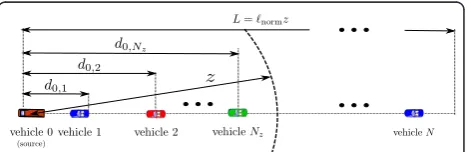
Figure 1 shows the linear network topology of reference for a generic multihop broadcast protocol: a static one-dimensional wireless network with a source and N (receiving) nodes. The assumption of static nodes is not restricting. In fact, from the perspective of a single transmitted packet, because of the very short transmis-sion time (with typical IEEE 802.11 transmistransmis-sion rates), the network appears as static [13]. At the same time, a one-dimensional network is suitable for analyzing
highway-like VANETs, where the width of the road (lying in the interval [10-40 m]) is significantly smaller than the transmission range of an IEEE 802.11 network interface. These motivations will be justified by simula-tion results in Secsimula-tion 7.
We consider a deterministic free-space propagation model (i.e., without fading) and a fixed transmit power: therefore, each vehicle has a fixed transmission range, denoted as z (dimension: [m]). The network size (the line length) is set to L(dimension: [m]). For generality, we denote as normalized network sizethe positive real numbernormL/z. Generally, ℓnorm> 1 and this
moti-vates the need for multihop communication protocols. On the basis of empirical traffic data [14], the nodes’ positions are generated according to a PPP of parameter rs, where rs is the vehicle (linear) spatial density
(dimension: [veh/m])–the symbol“veh” it is not a realis-tic unit of measure, but it will be used for the sake of clarity. Consequently, Nis a random variable character-ized by a one-dimensional Poisson distribution with parameterrsL. Similarly, the random variableNz,
denot-ing the number of nodes lydenot-ing in the transmission range of the source (e.g., within the interval (0,z)), has a Pois-son distribution with parameter rsz. Thanks to the
properties of the Poisson distribution, the inter-vehicle distance is exponentially distributed with parameterrs
and the (constant) average distance between two conse-cutive vehicles is 1/rs.
As shown in Figure 1, the source node, denoted as node 0, is placed at the west end of the network, and we assume a single propagation direction (eastbound). Each of the remaining Nnodes is uniquely identified by an index iÎ {1, 2,...,N}. The distance between the i-th andj-th nodes (i, jÎ{1, 2,...,N},i≠j) is denoted asdi,j.
Each vehicle can exactly estimate the value ofdi,j, thanks
to the following assumptions: (i) the position of the source is a-priori known by every node; (ii) each vehicle knows its own position under the assumption of the presence (on board) of a global positioning system (GPS) receiver; (iii) each rebroadcaster inserts its own geographical coordinates within the packet.
In the (one-dimensional and with a single propagation direction) scenario described in Figure 1, the operational principle of a multihop broadcast protocol is quite sim-ple. The initial transmission of a new packet from the source is denoted as the 0-th hop transmission, while the source itself identifies the so-called 0-thtransmission domain(TD). After the source transmission, the packet is then received by theNz source’s neighbors, that are
the potential rebroadcasters at the 1-st hop. Hence, their ensemble constitutes the 1-st TD. Each vehicle in the 1-st TD decides to forward the packet according to a PAF specified by the broadcast protocol. The use of
silencing corresponds to the fact that the “fastest” retransmitter (among the set of those which have decided to retransmit) silences the others. Note that a collision may happen if at least two nodes of a TD retransmit simultaneously. The propagation process is therefore constituted by multiple packet retransmissions, that continue at most till the east end of the network– as will be clear in the following, with a probabilistic broadcasting protocol the retransmission process might terminate before reaching the end of the network.
2.2 Performance metrics of interest
In this work, the performance of probabilistic multihop broadcast protocols will be investigated using the fol-lowing average metrics: (i) the REachability (RE), (ii) the transmission efficiency (TE), and (iii) the end-to-end delay (D). The RE (adimensional), originally introduced in [1], is the fraction of nodes that receive the source packet among the set of all reachable nodes. The cardin-ality of the set of the reachable nodes is denoted as nreach, and can be expressed as nreach = min(N, n*),
where n* is the minimum index such as the condition dn*, n* + 1 >z is verified. This definition is necessary
since in PPP scenarios, as those considered in this work, there can exist a pair of disconnected consecutive nodes (n*,n* + 1). The TE (adimensional) is defined as the ratio between the RE of a packet and the overall number of rebroadcast acts experienced during its transmission to the last reachable node. Finally, D (dim: [ms]) is defined as the duration of the packet trip between the source and the last reachable node. We remark that only the packets received correctly at the nreach-th node
of the network are considered for the evaluation of D. Therefore, this definition of D corresponds to a worst case scenario.
Owing to the symmetry of the forwarding process, the entire network can be modeled on the basis of the (local) analysis of a single TD. Therefore, in Section 3 we focus on a single TD–the reasons behind this assumption will be better clarified in Section 5.
3 Average distribution of poisson points in a segment with finite length
We now present a constructive definition of a PPP with parameterrs Î ℝ+, directly inspired from the one
pre-sented in [15, Ch. 3]. Given a finite interval (-T/2,T/2)⊂
ℝ, place n Î N points in (-T/2,T/2), under the con-straint thatn/T=rs. A PPP is obtained by lettingn®
∞ and T ® ∞, under the constraint that n/T remains equal tors. A PPP has the following properties: (i) the
finite interval I(0,z)⊂Ris a random variable with a Poisson distribution with parameter rsz. In Figure 2, an
illustrative realization of a PPP with parameter rs is
shown. With reference to Figure 2, denoting by n the number of Poisson points falling in I it is possible to define then-dimensional positions vector
R(n)= [R1R2...Rn] (1)
whereRi (iÎ {1, 2,..., n}) is the distance of the i-th
point from the source (placed in zero)–in the illustrative case in Figure 2,n= 2.
In Appendix 1, it is shown that the marginal probabil-ity densprobabil-ity function (PDF) ofRjis the following:
fR(nj)(r) =
⎧ ⎨ ⎩
n!
zn
(z−r)n−jrj−1
(n−j)!(j−1)! r∈(0,z) j= 1, ...,n 0 otherwise.
(2)
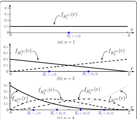
In Figure 3, the PDFs of the positions of consecutive nodes are shown for various values ofn: (a) 1, (b) 2, and (c) 4. In Appendix 1, it is also shown that the average position of thej-th node can be expressed as follows:
R(jn)=
z
0
rn! zn
(z−r)n−jrj−1
(n−j)!(j−1)!drj=j
z
n+ 1 j= 1, ...,n.(3) From Equation (3), it emerges clearly that, for a given number of nodes falling in a finite segment I, their average positions are equally spaced. The average nodes’ positions, for various values of the number nof nodes inI, are also shown in Figure 3.
Thanks to these results, the average performance analysis of a broadcast protocol in a network with Poisson node distribution can be carried out by simply studying a deterministic scenario, where the nodes are placed in correspondence to the average positions of the corresponding Poisson-based scenario. Moreover, this average analysis applies to other vehicle spatial distributions (e.g., taking into account the constraint on the vehicle lengths) with equally spaced average positions.
4 A quick overview of the IEEE 802.11b standard
In this work, we assume that the physical and the med-ium access control (MAC) layers of every node adhere to the IEEE 802.11b standard [16]. In this section, we first recall the basic features of this standard. Due to the broadcast nature of the communications, the contention channel is managed through the basic access (BA) mechanism, the operational principle of which can be briefly described as follows. When a node has a frame ready to be transmitted, it checks if the channel remains idle for a period of time at least longer than a distribu-ted interframe space (DIFS): if this is the case, the node is free to immediately transmit. On the opposite, if the wireless medium is busy, the node defers its transmis-sion until the medium remains idle for a whole DIFS without interruption. In the latter case, once the DIFS has elapsed, the node generates a random backoff per-iod, which corresponds to an additional waiting time before transmitting (pre-backoff). The node transmits when the backoff time has elapsed. At each transmission act, the backoff time is uniformly chosen in the range [0, cw -1], wherecwis the current backoff window size, that is constant and equal to the minimum value defined by the standard, denoted asCWmin, and
corre-sponding to 32. The backoff period is slotted and the duration of the backoff, expressed in terms of number of backoff slots, is denoted as backoff counter (BC). This number is decremented as long as the medium is sensed idle, and it is frozen when a transmission is detected on the channel (this is an instance of a colli-sion avoidance mechanism). Decrementing restarts when the medium is sensed idle again for more than a DIFS. At the end of every packet transmission, the node is forced to enter a post-backoff phase that coincides Figure 2 Illustrative realization of a PPP (the points
corresponds to X).
Figure 3The marginal distributions of the positions ofnnodes for various values ofn. The marginal distributions({fR(n)
i (r)}
with the subsequent pre-backoff if the node has another packet in the transmission queue.
It is important to observe that when a relay finds the channel idle, itcanimmediately transmit, but this is not mandatory. In order to reduce the number of collisions within a TD, we have interpreted the standard in a non-persistent manner, imposing that every relay enters into the pre-backoff phase, regardless of the channel status. We also remark that the extension of our approach to scenarios with IEEE 802.11p [17] communications, as envisioned in VANETs, is straightforward. Our approach (based on the IEEE 802.11b standard) is meaningful under the assumption of smartphone-based vehicular communications [18,19].
5 Probabilistic broadcast protocols with silencing 5.1 Preliminaries considerations
The general goal of a multihop broadcast protocol is to attain the widest network coverage in the shortest possi-ble time. This can be obtained by pursuing three inter-mediate goals: (i) minimizing the number of communication hops; (ii) minimizing the number of effective retransmissions in every hop; (iii) minimizing the latency associated with a single hop. The number of transmission hops can be minimized by designating, as relays, the nodes forming the MCDS. However, the number of retransmissions and the latency are directly affected by the protocol characteristics, and there is no general rule for minimizing them–this motivates the presence, in the literature, of a large number of heuristic broadcast protocols.
Aprobabilisticbroadcast protocol tries to achieve the goals outlined in the previous paragraph in a probabilistic and completely distributed manner: (i)probabilistic, in the sense that every intermediate node decides to retransmit a packet according to a certain PAF, com-puted on a per-packet manner–even if, in general, one could introduce a per-flow PAF, in this work we focus on single packet transmissions; (ii)distributed, in the sense that every node autonomously makes a retransmission decision without any coordination with its neighbors.
In“classical”probabilistic broadcast protocols (without silencing), without adopting suitable counter-measures it is possible that more than one node in a TD decides to rebroadcast the packet (even without collisions). This leads to inefficiencies–besides complicating the mathe-matical analysis. A more efficient probabilistic broadcast protocol, regardless of the expression of the PAF, is obtained in the presence of a single retransmitting node in every TD. This can be obtained by imposing that the reception of a packet sent by a node of a TD silences the preceding nodes of the same TD. As a consequence, the next TD starts from the node which follows the
“silencer.” Note that the last TD partially overlaps with the previous one if the“silencer” is not a member of the MCDS.
In this work, we consider two novel probabilistic broadcast protocols with silencing, whose operations can be described as follows, with respect to the first TD.
(1) The source sends a new packet (directly mapped on a IEEE 802.11 frame).
(2) The nodes within a distancez from the source receive the packet and form the 1-st TD. Their number is denoted asNz.
(3) Every node in the 1-st TD probabilistically deci-des, according to the given PAF and taking into account its distance from the source, to retransmit (or not) the packet.
(4) The potential forwarders (i.e., the nodes of the 1-st TD which have decided to retransmit) compete for channel access, by using the BA mechanism of the IEEE 802.11b standard (described in Section 4), first entering in the pre-backoff phase and, then, generating a random waiting time (denoted, in Sec-tion 4, as BC). For the purpose of analytical simpli-city, we assume that the BCs of the losing contenders are set to∞.
(5) The BCs are continuously decreased by all nodes, until (in the case of a successful forwarding) only one of them reaches 0, say thek-th BC. During a transmission of a node the other BCs freeze. Should there be the BCs of at least two nodes which reach simultaneously zero, both nodes would transmit and, thus, collide. We assume that the packets involved in a collision are considered undetectable and ignored by the other nodes. The correspondingk-th node retransmits the packet.
(6) The remaining Nz-1 nodes decode the packets,
reset their timers, and discard the potentially queued packet. The nodes (spatially) preceding the k-th node will refrain from retransmitting from then on. (7) The whole process (from Step 1) is restarted at the 2-nd TD, for which the k-th node acts as the source. The 2-nd TD is composed by all nodes lying in the interval (d0,k, d0,k +z) ⊂ℝ, and it can also
include some former nodes of the 1-st TD (those following thek-th node).
The two novel probabilistic broadcast protocols, poly-nomial and SIF, are described in the following two subsections.
5.2 Polynomial broadcast protocol
p(d,z,g)
d z
g
(4)
where: d denotes the distance (dimension: [m]) between the node of interest and the previous relay (or source, in the case of the first TD); z is the already introduced transmission range;gÎ Nis the polynomial order. According to the assumptions in Section 2, both z andd are assumed to be known without the need of exchanging additional messages. In fact,z can be esti-mated by knowing the transmit power and the channel propagation model, while dcan be estimated by simply inserting the position of the source vehicle in every transmitted packet (under the assumption of having an accurate GPS receiver).
The shape ofp, as a function ofd, is shown in Figure 4, for different values ofg. It can be observed that the functionpis monotonic and concave for all values ofg. For high values of g, it becomes quite “selective,”since it is approximately zero everywhere, but in the proxi-mity of z. Note that the case withg = 0 (p= 1,∀d) cor-responds to the flooding protocol, i.e., each node retransmits. In this case, the BC value is randomly selected in {0, 1,..., cw - 1} as mandated by the IEEE 802.11 standard (Section 4).
5.3 Silencing irresponsible forwarding
This broadcast protocol directly derives from the irre-sponsible forwarding (IF) protocol, originally presented in [20], with the introduction of the silencing mechan-ism with the introduction of the silencing mechanmechan-ism outlined in Section 5.2. Besides this difference, IF and
SIF share the same following PAF:
p(d,z,g)exp
−ρs
(d−z)
c (5)
where cis an adimensional shaping coefficient and rs
is the vehicle spatial density. The latter can be estimated in a straightforward manner. In fact, under the assump-tion of knowing with a sufficient accuracy its transmis-sion range, a node can estimate its local vehicular spatial density by simply counting the number of nodes lying within its transmission range and dividing them by the transmission range. The design of an efficient method for accurate estimation of the vehicular spatial density goes beyond the scope of this manuscript. How-ever, intuitively it is sufficient to periodically send (and receive) Hello messages to the surrounding nodes. Alter-natively, it is possible to rely on already existing beacon-ing mechanisms, such as the exchange of cooperative awareness messages (CAMs) foreseen by the European car-to-car consortium (broadcasted by default every 500 ms) [21].
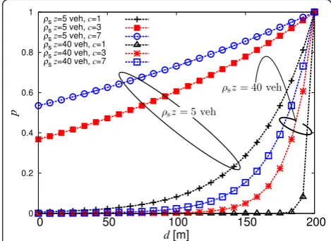
Similarly to the PAF of the polynomial broadcast pro-tocol, also the PAF of SIF “rewards” the farthest nodes (with respect to the transmitter). However, unlike the polynomial PAF, the PAF of SIF also takes into accounts the (linear) vehicular spatial density, thus allowing to better adapt to different traffic conditions– this is the very idea of IF. The shape of p, as a function of d, is shown in Figure 5, for different values of c and rs. It
can be observed that the PAF of SIF is monotonically increasing and concave for all values ofc. Moreover, it becomes selective far small values of c(e.g., 1), while it tends to flatten for high values ofc and for low values of rs. Also in this case, the BC value is randomly
0 0 0.2 0.4 0.6 0.8 1
Figure 4Probability of retransmission (denoted asp) of the polynomial probabilistic protocol as a function of the distance
dfor several values ofg.
0 0.2 0.4 0.6 0.8 1
0 50 100 150 200
[m]
ρs=5 veh, =1 ρs=5 veh, =3 ρs=5 veh, =7 ρs=40 veh, =1 ρs=40 veh, =3 ρs=40 veh, =7
Figure 5Probability of retransmission (denoted asp) of the SIF
protocol as a function of the distancedfor several values ofc
selected in {0, 1,..., cw - 1} as mandated by the IEEE 802.11 standard (Section 4).
6 A recursive analytical performance evaluation framework
In Section 2, it has been stated that, since all TDs are statistically identical, the global behavior of the network can be modeled by analyzing a single TD. By exploiting the properties of probabilistic broadcast protocols with silencing (described in Section 5), the following assump-tions hold: (i) the inter-node distance is characterized by a (memoryless) exponential distribution, so that the topology of every TD is (statistically) identical; (ii) the PAF only depends on the distance and is, therefore, memoryless; (iii) the IEEE 802.11b contention mechan-ism is memoryless, in the sense that it is restarted at every retransmission. Under these assumptions, every retransmission act can be interpreted as a renewal that resets the statistics of the forwarding process. Moreover, since all TDs are statistically identical, without loss of generality we can focus on the first TD.
Therefore, a complete analytical performance evalua-tion framework can be derived in the following manner: (i) characterizing the first TD withlocal performance metrics (e.g., the successful transmission probability and the delay); (ii) derivingglobalperformance metrics (e.g., D, RE, TE), by means of a recursive approach.
In Section 6.1, the local performance (i.e., single TD) is investigated under the assumption of a given number of equally spaced nodes, by considering, without loss of generality, the first TD. In Section 6.2, we derive the global metrics for an overall deterministic network sce-nario, where the nodes are equally spaced in the interval (0,L). Then, in Section 6.3 the results obtained in the deterministic scenario are extended to the original PPP-based scenario.
6.1 Local (single TD) performance analysis with a given number of nodes
Without loss of generality, we focus on the first TD, corresponding to the interval I introduced in Section 3. We consider a deterministic scenario with a fixed number n of nodes equally spaced in the interval
I= (0,z)⊂R. Every node in a TD is identified by an index i Î {1, 2, ..., n}. The nodes are thus positioned as in Figure 3 and the positions vector R(n)is defined as in (1).
According to the operational principles of the consid-ered protocol, after the reception of a packet in a given TD, each node decides to (or not to) retransmit accord-ing to the protocol’s PAF. The nodes that lose the con-tention set their BCs to∞, while the winners set their BCs according to the policy of the specific broadcast
protocol. The protocol execution could lead to three dif-ferent outcomes: (i) nobody decides to retransmit; (ii) some nodes decide to retransmit, but all their trans-mitted packets collide; (iii) some nodes decide to retransmit, and a single node transmits successfully (when its BC because zero, no other BC is zero). It is useful to define the following events, associated to the forwarding process in a TD:
F1{nobody decides to retransmit} ={BCi=∞, ∀i∈ {0, 1, ...,n}} F2{all the transmitted packets collide}
={∀i∈ {0, 1, ...,n}: BCi<∞,∃j∈ {0, 1, ...,n},j=i, BCj<∞such as BCi= BCj} F{nobody wins the contention}=F1∪F2
Si{the nodeisuccessfully retransmits} i∈ {1, ...,n} ={BCi<∞, BCi= min({BCm}nm=1)
∪ {if∃j∈ {1, ...,n},i=j: BCj<BCi, then∃m∈ {1, ...,n},m=j,m=i: BCj= BCm} i∈ {1, ...,n}
S{a node successfully retransmits}= n
i=1 Si
The probabilities of the above defined events are the following:
p(rtxn)(i)P{Si} i= 1, 2, ...,n
p(succn) P{S}=
n
i=1 p(rtxn)(i)
p(failn)1−P{S}= 1−
n
i=1 p(rtxn)(i).
Let us now introduce the random variable YÎ {0, 1, 2, ... ,n} with the following PMF:
PY(y) =P{Y=y}=
p(failn) y= 0 p(rtxn)(y)y∈ {1, 2, ...,n}.
Since the event {Y= 0} identifies the failure event, the random variableYindicates either which node has effec-tively retransmitted or a failure. Moreover, it can be observed that:
n
y=1
{Y =y}=F∪S.
Obviously,
PY(y|S) =PY(Y=y|S) = ⎧ ⎪ ⎨ ⎪ ⎩
0 y= 0
p(rtxn)(x)
n
t=1p
(n) rtx(i)
y∈ {1, 2, ...,n}.
In other words, if there is a retransmission (S), then
PY(y|S) (y∈ {0, 1, 2, ...,n})is the probability that the
y-thnode has retransmitted.
p(rtxn)(i) =pi
node and depends on the considered protocol; q(m)is the probability that thei-th node wins the contention among a set of m competing nodes (the same for a given value of n);Vi(n)∈ {0, ...,n−1}is the following discrete random variable:
V(in){number of nodes, among thennodes, competing with thei−th node}.
The derivation ofq(m)and of the PMF ofVi(n)can also be found in Appendix 2.
After deriving p(n)
rtx(i), it is possible to compute the per-hop delay, denoted asDi, of a retransmission from
the i-th node. Since the per-hop delay is meaningful only if thei-th node decides to retransmit, it is of inter-est to study the statistical distribution ofDi conditioned
onSi. For this reason, we introduce the random variable
Di|i, which can be defined as follows: Di|iTslot(DIFS+Nibo|i) +T
tx
i= 1, ...,n
where:Ttx (dimension: [s]) is the transmission time; Tslot (dimension: [s/slot]) is the deterministic duration of
the backoff slot; DIFS(dimension: [slot]) is the duration of the DIFS; andNboi|i (dimension: [slots]) is the number of slots spent by thei-th node during thebackoff (condi-tionally on the event Si). We assume that both the
packet size, defined as P (dimension: [bits]), and the transmission rate, denoted asR(dimension: [bits/s]), are constant, thus leading to a deterministic packet trans-mission timeTtx =P/R. Taking into account that DIFS,
where, according to the derivation in Appendix 3,
Nboi|i=
(v/2))denotes the maximum number of collisions that can happen in slots 0, 1, ..., k -1, while the matrixPv={Pv(k,j)}is defined in Appendix
3.
Proceeding in a similar manner, it is also possible to obtain the average number of retransmissions per-hop of the nodei, denoted asNhoprtx (i):
h) are defined in Appendix 3.
6.2 Global performance analysis with fixed number of nodes
Once the per-TD performance has been analyzed (as described in Section 6.1), the global performance metrics introduced in Section 2.2 (namely, RE, TE, and D) can be computed by following a recursive approach, based on the inductive principle. This recursive approach is extensively described, for the evaluation of D, in Appendix 4, but can be directly re-adapted for the evaluation of RE and TE. In the remainder of this sub-section, we outline the final results, trying to provide the reader with the intuition behind them.
Recall that we consider a deterministic scenario with a fixed number Nof nodes equally spaced in the interval (0,L)⊂ℝ, whereL=zℓnorm. For simplicity, we assume
that a generic TD containsn=N/ℓnormnodes. This
cor-responds to a best-case scenario, where the farthest node of each TD is the domain forwarder (the “ silen-cer,”as denoted in Section 5).
DelayThe computation of the average D is carried out taking into account only the packets successfully arriv-ing at the end of the network (i.e., at the last reachable node) and ignoring the (remaining) packets which stop earlier. On the basis of the approach described in detail in Appendix 4, the average end-to-end delay can be given the following recursive formulation:
DD(N)=Ttxsrc+ - i nodes and Ttxsrcis the average transmission time of the source, which differs from those of the following nodes, since the source does not contend with any other node and its transmission is not affected by collisions. Since the average time spent in the backoff is Ttxsrc can be expressed as
REThe average RE can be defined as follows:
RE Nreach
where Nre a c h is a random variable denoting the
number of nodes reached by a packet. As a conse-quence of our assumptions, Nreach is lower bounded
by n, since the transmission from the source reachesn nodes (those of the first TD) with probability 1. The average value Nreachcan be obtained by following the approach described in Appendix 4, but for the repla-cement of pY(i|S)withpY(i) and of Di|iwith the
num-ber of additional nodes covered by a new transmission. For example: a transmission from the 1-st node of the fir1-st TD will reach only one additional node (namely, the (n + 1)-th); a transmission from the 3-rd node will reach three additional nodes (namely, the (n + 1)-th, (n + 2)-th, and (n + 3)-th); and so on. Please note that, unlike the delay, in the computation of the RE we are not conditioning on the fact of reaching the N-th node of the network, i.e., the last reachable node of the network. Therefore, also the packets which stop being retransmitted are taken into account.
After the execution of the recursive approach outlined in Appendix 4, it is sufficient to add a constant equal to n, corresponding to the number of nodes directly reached by the source at the first hop. The final expres-sion ofNreachbecomes (using the notation of Appendix 4):
Nreach=N (N) reach=n+
n
i=1
N(reachN−i)+ipY(i)
=n+
n
i=1
N(reachN−i)+ip(rtxn)(i)
(13)
where N(reachN−i)corresponds to the average number of nodes reached in a network withN- inodes and can be recursively computed in the same way.
TEIn order to reduce the computational burden, we adopt the following approximated formulation of TE:
TE RE Nrtx
(14)
where Nrtx denotes the average overall number of retransmissions over all hops. From a computation view-point Nrtx is approximated by Nm
(∗)
rtx , where m* corre-sponds to the average number of reached nodes-it is a sort of approximated indicator of the“depth”of the pro-pagation process. Since the RE can be interpreted as the ratio between the average number of reached nodes and the total number (N) of nodes, m* can be approximated as follows:
m∗ N·RE.
At this point, Nm(∗)
rtx can be computed by applying the recursive approach presented in Appendix 4, by repla-cing (i)pY(i|S)withpY(i) and (ii)Di|iwith the average
number of transmissions per hop, denoted by Nhop rtx and given in (9).
6.3 Generalization to a PPP-based scenario
According to the original PPP-based model, described in Section 2, the number of nodes within I, denoted asNz,
has the following Poisson distribution:
pNz(n,ρsz) = e−ρsz(ρ
sz)n
n! n∈ {0, 1, 2, ...}.
However, since a real vehicle has a finite length, it is not possible to have an infinite number of vehicles within I. Therefore, it makes sense to impose an arbi-trary limit to the maximum number of nodes within I, denoted asNc. The new truncated Poisson random
vari-able, denoted asNz, has the following distribution:
pNz(n,ρsz) =
e−ρsz(ρ
sz)n n! Nc
i=1 e−ρsz(ρ
sz)i i!
n∈ {1, 2, ...,Nc}
where we have also removed the event n = 0–this would correspond to an empty TD.
In order to exploit the results of Section 6.1, the sto-chastic network topology of the PPP needs to be mapped into a deterministic one with equally spaced nodes. In order to do this, the interval I is partitioned in Nint sub-intervals of lengthz/Nint, whereNintÎ {Nc,
Nc + 1,Nc+ 2,...} is a design parameter. The
computa-tional burden and the accuracy are directly related to the value of Nint. After some numerical tests, we observed that the valueNint = 100 is a good tradeoff between precision and computational time. The i-th sub-interval thus is:
Ii=
(i−i)z
Nint , iz Nint
i= 1, 2, ...,Nint .
Every sub-interval can contain at most one node: in general, we assume that in each sub-interval there is a “virtual”node. Consequently, it is possible to associate a transmission probability peqrtx(i)to the generic sub-inter-val Ii, defined as peqrtx(i), and a corresponding per-node delay, denoted asD(i)eq(i= 1,...,Nint).
We define as p(rtxn)(j)the probability of retransmission of thej-th node, given that there are exactlynnodes in the interval I. Using the total probability theorem,
peqrtx(i) =
Nc
n=1
(peqrtx(i)|Nz=n)P(Nz=n)
=
Nc
n=1
n
j=1
p(rtxn)(j)f(i,j,n)pNz(n,ρsz)i∈ {1, ...,Nint }
(15)
where f(i,j,n) is an indicator function defined as fol-lows:
f(i,j,n)
1 R(jn)∈Ii
0 R(jn)∈/ Ii.
(16)
The probabilitypeqrtx(i)is now a function ofp(rtxn)(i)(nÎ {1, 2,..., Nc}, i Î {1, 2,..., n}), which can be computed
with combinatorics, since it is associated with a determi-nistic scenario withnstatic nodes equally spaced in [0, z].
At this point, by using (6) in Equation (15), it is possi-ble to obtain a closed-form expression forpeqrtx(i). Lever-aging on the knowledge of peqrtx(i), by using Equations (15) into (7) and (9), it is possible to obtain, respectively, D(i)eq(i= 1,...,Nint) andnhoprtx eq. Then, it is possible to use the framework presented in Section 6.2 to derive RE, TE, and D for a deterministic network composed by Ncℓnorm nodes, since Nc is the (imposed) number of
nodes in the interval I (and, thus, in each TD).
As anticipated at the end of Section 1, we remark that the presented analytical framework can be employed to study other types of broadcast protocols, not necessarily probabilistic, by simply re-adapting the definition of
p(rtxn)(i) and Di|i. This is the subject of our current
research activities.
7 Theoretical performance analysis and simulation-based validation
7.1 Polynomial protocol
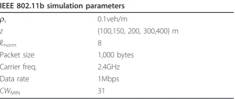
In this section, we compare the results obtained with the analytical framework presented in Section 6 with results obtained through numerical simulations carried out with the ns-2.34 simulator [22]. In particular, the polynomial protocol has been“inserted” on top of the IEEE 802.11b model, after fixing the bugs reported in [23]. We observe that, conditionally on the fact of suita-bly scaling the packet size and the packet generation rate, from the perspective of our framework the IEEE 802.11a/p standards will offer the same performance of the IEEE 802.11b standard. All the results presented are accurate within ±5% of the values shown with 95% con-fidence. The relevant parameters of the simulation are listed in Table 1. The results are obtained for a fixed node spatial densityrs = 0.1 veh/m, while the possible
values of the transmission rangezare listed in Table 1. In particular, the values of z are selected so that the
corresponding values of rsz are between 10 and 40veh.
In the numerical simulations, we do not consider any case withrsz< 10 veh, since this corresponds to
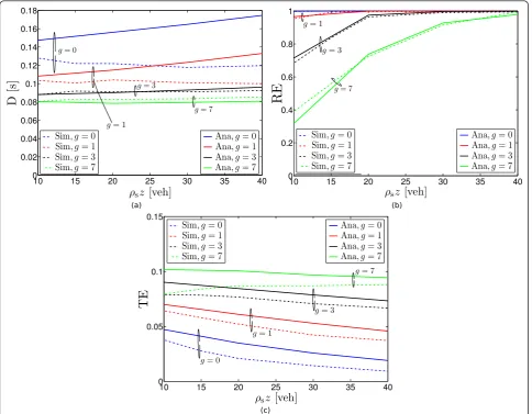
topolo-gies that are disconnected with a high probability, as shown in [10]. In Figure 6, (a) D, (b) RE, and (c) TE are shown as functions of rsz, for different values ofg, by
taking into account both the results of the analytical fra-mework and of the numerical simulations, thus allowing to assess the validity of the analytical model. As shown in [10], using the considered values of rsz (between 10
and 40 veh), the network is fully connected (i.e.,nreach=
N) with a high probability. From Figure 6b it emerges that, in terms of RE, there is an excellent match between the results of the theoretical framework and those of the simulator. As shown by Figure 6c, the agreement between analysis and simulations is still good also in terms of TE. On the other hand, the delay pre-dicted by the analytical framework overestimates the true delay for small values of g(e.g., g = 0), whereas it becomes very accurate for large values ofg (e.g.,g = 7). The comparative investigation of analytical and simula-tion results indicates the validity of the proposed frame-work (especially for large values ofg).
According to the results in Figure 6a,c, it emerges that a higher polynomial degree leads to a better perfor-mance, regardless of the value ofrsz, in terms of both D
and TE. Conversely, since the PAF is highly selective for large values of g (as shown in Figure 4), this leads to poor performance in terms of RE, as shown in Figure 6b. By considering small values ofg (e.g.,g = 0 corre-sponds to flooding), one observes the opposite phenom-enon: a drastic improvement in terms of RE, at the price of a slightly higher D and a smaller TE.
In order to better understand the impact ofgandrsz
on the protocol performance: in Figure 7a, D is shown, parametrized with respect tog, as a function of RE for different values of rsz; while in Figure 7b D is shown,
parametrized with respect torsz, as a function of RE for
different values of g. From the results in Figure 7a, it emerges that even little variations ofg lead to radically different protocol behaviors. On the contrary,rszhas an
impact on the performance only for small values ofrsz,
Table 1 Main IEEE 802.11b network simulation parameters
IEEE 802.11b simulation parameters
rs 0.1veh/m
z {100,150, 200, 300,400} m
ℓnorm 8
Packet size 1,000 bytes Carrier freq. 2.4GHz
Data rate 1Mbps
while for increasing values of rsz (e.g., larger than 20
veh) its impact vanishes.
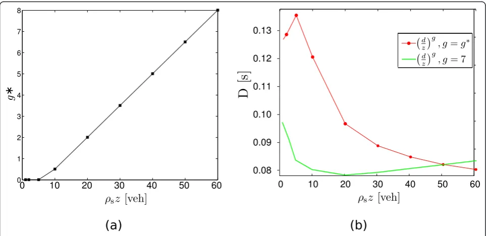
From the results in Figures 6 and 7, it emerges clearly that there is no optimal value of g. However, the pro-posed framework allows to optimize a single perfor-mance metric, after having imposed some constraints on the other metrics, on the basis of proper quality of ser-vice criteria. A possible choice consists in ignoring TE and minimizing D under the constraint of attaining a target value of RE. Since D is a decreasing function ofg, it is possible to define the following quasi-optimalg*:
g∗(ρsz) ={max(g)|RE(ρsz)>0.95}.
Selectingg=g* allows to achieve the minimum delay under a constraint on the RE. The obtainedg* is shown, as a function ofrsz, in Figure 8a, and the following
considera-tions can be drawn: (i) g* is an increasing monotonic
function ofrsz; (ii) with the exception of the region in
proximity torsz= 0, whereg* tends to 0,g* has a
quasi-lin-ear dependence with respect torsz. It can be shown that if RE1for each value ofrsz. Note that the selection ofg*
allows to maximize RE. However, as shown in Figure 8, D is always higher than 0.08s, a delay which is instead guar-anteed by the use ofg= 7, as shown in the same figure.
7.2 Silencing irresponsible forwarding
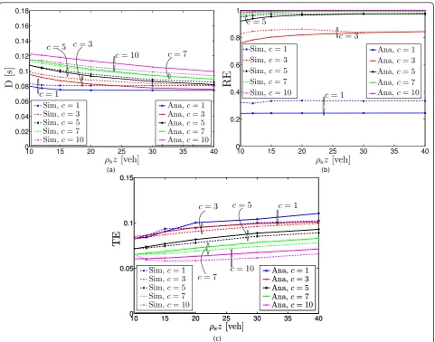
As pointed out in Section 6, the proposed framework can be applied to a large family of broadcast protocols. In this section, the framework is applied to SIF. In parti-cular, the validity of the proposed analytical framework is clearly shown in Figure 9, where (a) D, (b) RE, and (c) TE are shown, as functions ofrsz, for different values of
c, by directly comparing both analytical and simulation results. As with the polynomial broadcast protocol, in
10 15 20 25 30 35 40
0 0.02 0.04 0.06 0.08 0.1 0.12 0.14 0.16 0.18
10 15 20 25 30 35 40
0 0.2 0.4 0.6 0.8 1
10 15 20 25 30 35 40
0 0.05 0.1 0.15
Figure 6Simulation and analytical performance results of the polynomial protocol. (a) D,(b)RE, and(c)TE, as a function ofrsz, obtained
this case as well there is a good agreement between the results obtained with the analytical model and the simu-lations. In particular, it can be observed that the accu-racy of the model depends on the value of the shape parameter c (the highest average accuracy, over all metrics, is observed withc= 7). By comparing Figures 6 and 9, one can observe that polynomial and SIF proto-cols have a different dependence onrsz. In particular, in
the case of SIF, as the productrszincreases RE remains
roughly the same, while D decreases and TE increases.
In other words, SIF performs better in dense networks. On the other hand, in the case of the polynomial proto-col (Figure 6), D and TE have an opposite behavior (namely, D slightly increases and TE slightly decreases for increasing values of rsz), and RE strongly depends
on rsz, especially in sparse networks. In general, SIF
outperforms the polynomial broadcast protocol.
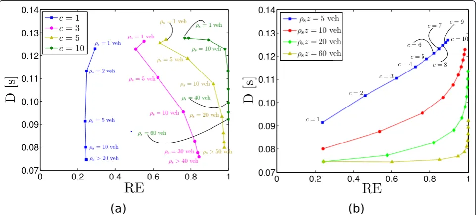
Furthermore, from Figure 9 it is clear that also for SIF there is no optimal value of the parameter c which simultaneously optimizes the performance according to
0.1 0.2 0.3 0.4 0.5 0.6 0.7 0.8 0.9 1
0.06 0.08 0.1 0.12 0.14 0.16 0.18
0.1 0.2 0.3 0.4 0.5 0.6 0.7 0.8 0.9 1
0.08 0.09 0.1 0.11 0.12 0.13 0.14 0.15 0.16 0.17
Figure 7Analytical performance results of the polynomial protocol. D as a function of RE, parametrized with respect to (a)rsz(for various values ofg) and (b)g(for various values ofrsz). The results are obtained by consideringCW= 31,lnorm= 8,P= 1000 bytes, andR= 1 Mbps.
0 10 20 30 40 50 60
0.08 0.09 0.10 0.11 0.12 0.13
0 1 2 3 4 5 6 7 8
0 10 20 30 40 50 60
all considered metrics. This fact can be better under-stood from Figure 10, where D is shown as a function of RE, parametrized, respectively, with respect to (a) rsz
and (b)c. In particular, from Figure 10b it emerges that if one wants to guarantee a minimum value of RE (say 0.95), it is necessary to use a sufficiently high value of c. This, in turns, does not minimizeD, which, as shown in Figure 10b, is directly proportional toc. Moreover, the results in Figure 10a strengthen the observations carried out regarding the results in Figure 9. In fact, they clearly evidence two important characteristics of SIF: (i) RE is not affected by the value of rsz, as SIF automatically
adapts; (ii) counterintuitively D is a decreasing function ofrsz(e.g., SIF performs better in dense networks). 7.3 Comparison with benchmark protocols
As aforementioned, the theoretical framework presented in this manuscript can be used for evaluating a large
number of broadcast protocols. In this subsection, it is applied to two benchmark broadcast protocols: (i) the flooding protocol (denoted with“FLOOD”), where each node forwards a received message; (ii) the optimal MCDS-based protocol (denoted with“MCDS”), where a hypothetical network genius selects as relays only the nodes belonging to the MCDS set (as described in Sec-tion 1). In both cases, the silencing mechanism is employed.
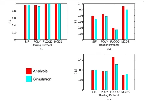
These benchmark protocols are compared with the SIF and polynomial protocols, considering a vehicle spa-tial distribution characterized by a Poisson distribution with parameterrsz = 16veh. In order to have a
signifi-cant comparison, the optimal values ofcandg(c* = 4.8 and g* = 2.7) are considered. These values, obtained through the analytical framework, allow to minimize D under the constraint of having a RE higher than 0.95, in a scenario with rsz = 16veh. The results, attained
10 15 20 25 30 35 40
0 0.02 0.04 0.06 0.08 0.1 0.12 0.14 0.16 0.18
10 15 20 25 30 35 40
0 0.2 0.4 0.6 0.8 1
10 15 20 25 30 35 40
0 0.05 0.1 0.15
10 15 20 25 30 35 40
0 0.05 0.1 0.15
through both simulations and theoretical analysis, are shown in Figure 11. From the results in Figure 11, a few considerations can be drawn. First, for all considered metrics, there is a performance loss between the MCDS-based and the optimized SIF/polynomial proto-cols. At the same time, the SIF/polynomial protocols exhibit a similar performance gain with respect to flood-ing (with the exception of the RE metric). It is also pos-sible to observe that, counterintuitively, the SIF and the polynomial protocols offer a similar performance level. This result can be motivated by considering that their PAFs tend to converge to a common shape, when using, respectively, the optimal values g* and c* as their key parameters. Finally, it can be also be noticed an excel-lent match between simulation and theoretical results can be observed.
7.4 Impact of topology on the protocol performance
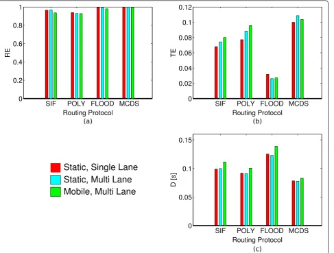
The goal of this subsection is to assess (a-posteriori) the validity of the assumption, made in Section 2, of consid-ering auni-dimensional staticnetwork. The validation is performed through simulations, by taking into account the protocols considered in Section 7.3 (namely, flooding, MCDS-based, SIF, and polynomial protocols). According to our assumption, we expect that the performances offered by these protocols will not be significantly affected by the network topology. To this end, we con-sider three different scenarios: (i) the uni-dimensional (single-lane) static network presented in Section 2; (ii) a multi-lane static network; (iii) a multi-lane mobile net-work. The multi-lane static scenario is composed by
Nlane= 6 adjacent lanes, each with width equal towlane=
4 m. This network is obtained by simply replicating the single-lane topology. In particular, in each lane the posi-tions of the vehicles are generated according to a PPP of parameterrs/Nlane. Similarly, the multi-lane mobile
sce-nario is composed by Nlane= 6 adjacent lanes (3 per
direction of movement), each with width equal towlane=
4 m. In this case, the vehicles are moving according to the intelligent driver motion with lane changes (IDM-LC) mobility model [24] and, therefore, their positions do not have Poisson distribution. The mobility traces have been obtained using VanetMobiSim [25] and plugged in the ns-2 network simulator. The vehicles’ speeds are independent and uniformly distributed in the interval (20-40) m/s. Greater insights about the mobility models and the trace generation process are provided in [26]. It should be noticed that the value of the per-lane vehicular density (rs) is time-averaged, since it is computed directly
from the mobility trace and thus is time-varying. In Fig-ure 12, we show the results obtained by consideringrs=
16 veh and the optimal values ofcandg(c* = 4.8 andg* = 2.7). It can be easily noticed that the performances obtained in the considered scenarios are quite similar. Hence, this proves (a-posteriori) that the assumptions made in Section 2 are substantially correct. More specifi-cally, it can be observed that increasing the width of the network leads to very similar values of RE and D, and to slightly higher TE (this can be justified by considering that there is a higher number of nodes in the neighbor-hood of a vehicle). Instead, if we consider the same sce-nario but with mobile vehicles, one can observe that the
0 0.2 0.4 0.6 0.8 1
0.07 0.08 0.09 0.10 0.11 0.12 0.13 0.14
0 0.2 0.4 0.6 0.8 1
0.07 0.08 0.09 0.10 0.11 0.12 0.13 0.14
Figure 10Simulation and analytical performance results of the SIF protocol. (a) D,(b)RE, and(c)TE, as a function ofrsz, obtained using
RE becomes slightly lower, while D and TE become higher. This behavior is motivated by the tendency of mobile VANETs to form ephemeral clusters of vehicles [27], leading to a reduced RE and increased D but to a higher TE.
Finally, the limited impact of the vehicle mobility on the protocols’performance could have been expected by considering the values of the worst case transmission time (about 0.2 s) and of the the maximum allowed speed (roughly equal to 40 m/s, corresponding to 144km/h). In these conditions, two vehicles proceeding in opposite directions on a highway have a differential speed of 80 m/s, and this leads, in turn, to a distance variation of 16 m during a packet transmission time. A distance of 16 m (the worst-case variation) corresponds to a small fraction of the transmission range of a typical IEEE 802.11 network interface (in Figure 12, we have consideredz= 160 m).
8 Conclusions
In this article, we have presented a theoretical frame-work, based on a recursive computational approach,
for average performance analysis of multihop broadcast protocols with silencing. We have then considered its application to VANET scenarios. The framework can be used in all the scenarios where the nodes’positions are distributed in such a way that their average posi-tions are equally spaced. For example, it can be readily used for topologies where the nodes’ positions have approximately a Poisson distribution. The proposed framework can be applied to a broad family of proto-cols and its validity has been assessed by means of ns-2 simulations, by considering several VANET scenar-ios. In particular, the framework allows to characterize the average performance of broadcast multihop proto-cols in highway-like scenarios, either static or mobile, thus preventing the use of time-wasting numerical simulations.
Appendix 1: Derivation of the average nodes positions
In this appendix, we derive the average value of the positions vector R(n) (n Î N) of nPoisson points fall-ing in the finite interval I= (0,z). The average values
TE
SIF POLY FLOOD MCDS
0 0.05 0.1 0.15
Routing Protocol
D [s]
SIF POLY FLOOD MCDS
0 0.2 0.4 0.6 0.8 1
Routing Protocol
RE
SIF POLY FLOOD MCDS
0 0.02 0.04 0.06 0.08 0.1 0.12
Routing Protocol
can be computed by firstly deriving the joint PDF of the vectorR(n), denoted as fR(n)(r), and defined over a proper n-dimensional domain Dn. From fR(n)(r), it is
then possible to derive the marginal PDF of Rj (j = 1,
2,..., n), denoted as fR(nj)(rj)and, from this, the average
valueR(jn).
A single point in I
In this case, n = 1 and Dn=I. In this case, R1 has a
uniform distribution in I and its (marginal) PDF is given by:
fR(1)1 (r1) = 1
z r1∈D1 0 otherwise.
The average value is:
R(1)1 = z 2.
Two points inI
Without loss of generality, it is possible to order the points by imposing thatr2 >r1. Thanks to this
assump-tion,D2can be expressed as follows:
D2={(r1,r2)∈R2:r1∈(0,z),r2∈(0,z),r1<r2}.
The joint PDF is uniform over D2 and can be expressed as follows:
fR1R2(r1,r2) = ⎧ ⎨ ⎩
1 Area(D2)
(r1,r2)∈D2
0 otherwise
= 2
z2 (r1,r2)∈D2 0 otherwise
SIF POLY FLOOD MCDS
0 0.2 0.4 0.6 0.8 1
Routing Protocol
RE
SIF POLY FLOOD MCDS
0 0.02 0.04 0.06 0.08 0.1 0.12
Routing Protocol
TE
SIF POLY FLOOD MCDS
0 0.05 0.1 0.15
Routing Protocol
D [s]
Static, Single Lane
Static, Multi Lane
Mobile, Multi Lane
Figure 12Simulation analysis of the impact of the network topology on the performance of several protocols. (a) D,(b)RE, and(c)TE, obtained using the SIF, polynomial, flooding, and MCDS protocols, withrsz= 16 veh,c* = 4.8, andg* = 2.7. The results are obtained through
From the joint PDF, the marginal PDFs ofR1 andR2
Using Equations (17) and (18), the average values of R1andR2 can be expressed:
A generic number ofnpoints inI
As in the case with n = 2, it is possible to order the points as that r1 <r2< · · · <rn, without losing any
gen-erality. Hence, the n-dimensional domain can be expressed as follows:
Dn={(r1, ...,rn)∈Rn:ri∈(0,z)∀i∈ {1, ...,n},r1<r2<· · ·<rn}.
The joint PDF of the nPoisson points has the follow-ing expression:
The marginal PDF of the position of thei-th point is given by:
On the basis of Equation (19), it is straightforward to derive the marginal PDF of Ri(i= 1, 2, ...,n), given the
presence ofnpoints in the intervalI:
fR(ni)(ri) =
Finally, from Equation (20) the average value ofRican
be expressed as follows:
R(in)=
Appendix 2: Per-node retransmission probability in a network with equally spaced nodes
We consider the deterministic scenario introduced in Section 6.1, composed by a fixed number n of nodes equally spaced in the interval I= (0,z)⊂R, with the positions vector R(n) defined in Equation (1). In this appendix, we derive the following probabilities:
where the eventSiwas defined in Section 6.1. In order
to derivep(rtxn)(i), it is helpful to introduce the following auxiliary events:
•Bi{the nodeiis designated as a relay};
• Ci{the nodei wins the contention among a set
ofnnodes}; •D(m)
i A {the nodeiwins the contention among a
set ofmcontending nodes};
• Wk {the value BC = k is chosen by a single
node}k= 0,...,cw- 1;
•W{at least a value of BCÎ[0, cw- 1] is chosen by a single node}.
The event Si, defined in Subsection 6.1, is verified if
both the eventsBiandCihappen. Therefore,p(rtxn)(i)can
be expressed as:
p(rtxn)(i) = P{Si}= P{Bi∩Ci}= P{Bi}P{Ci}
where the last equality is motivated by the indepen-dence of the eventsBiand Ci. The probabilityP{Bi}is
known, since it should be replaced with one of the PAF used by the protocols considered in this work (defined in Equations (4) and (5)). On the opposite, the unknown probabilityP{Ci}can be derived by applying the total
probability theorem, thus obtaining:
p(rtxn)(i) =P{Bi}P{Ci}
discrete random variable defined as:
V(in){the number of nodes competing with nodeigivennnodes}. the BA mechanism of the IEEE 802.11b standard. In
particular, it emerges thatq(m)(i) is independent ofiand can be expressed as follows:
q(m)(i) =q(m)= P{W}
Since the events{Wk}are not disjoint, it is necessary
to use the generalized union probability formula [29, Ch.4] to computeP{W}:
Since the addenda of each single sum of the right-hand side of (22) are the same, taking into account the number of possible combinations, the generic right-hand side of (22) can be then expressed as follows:
(−1)r+1
Thanks to Equation (22),q(n)can be finally given the following expression:
where the term min (n, cw) is introduced to deal with the casen<cw.
Appendix 3: Per-node delay in a network with equally spaced nodes
In this appendix, we derive the number of slots spent by the i-th node during the backoff conditioned to the eventSi, denoted as Nboi|i. By analyzing the BA
mechan-ism of the IEEE 802.11b standard, one obtains:
Nboi|i =E
can be derived by means of the Bayes theorem as follows:
Instead,E
can be derived by obser-ving that the delay associated with the event {the nodei transmits with success givenvcontending nodes} depends on two factors: (i) the slotBCiÎ{0,...,cw-1} selected by
the nodeifor transmitting; (ii) the number of collisions occurred in the slots 0,...,k- 1, which, given thatBCi=k,
corresponds to the following random variable:
Ncolk,v={number of collisions in slots 0,. . .,k−1}N
col
k,v∈ {0,Jk,v}
where Jk,v min(k,
(v/2))denotes the maximum number of collisions that can happen in slots 0,...,k-1. On the basis of these considerations it can be shown that:
E+Nbo
In order to derivePvit is necessary to define the
fol-lowing random variables:
orem and the total probability theorem:
Pv(k,j) = P{BCi=k∧Ncolk,v=j|V
In order to reduce the computational burden, the matrix
Mk,vcan be derived by means of a recursive strategy. In
particular, it can be observed that the number of collisions at thek-th hop is identical to (if nobody select the value BC =k- 1) or greater than 1 (if at least two nodes selects that value). Hence, once derived M1,vit is possible to
determineMk,vfor all the remaining values ofk. In
parti-cular, the direct formulation fork= 1 is the following:
M1,v(j,h) =
from which it is possible to derive Mk+1,v for any
values ofk:
where the indicator functionIj,kis defined as
Ij,k
1j=k 0j=k.
Finally, using Equations (24) and (25) in (23), one obtains the final expression:
This allows to determineDi|ifor every node of a given
TD.
Appendix 4: Recursive approach for the evaluation of the performance global metrics
In this appendix, we outline the recursive approach which, coherently with an inductive principle, allows to derive the average global performance metrics (namely, RE, D, and TE), on the basis of the average local perfor-mance metrics of a generic TD. We recall that, thanks to the assumptions of the deterministic approach, all the TDs are identical and composed of nnodes. The recur-sive approach is detailed by considering the computation of D, but with the same approach it is also possible to derive RE and TE. The computation of the average D is carried out taking into account only the packets success-fully arriving at the last reachable node, ignoring the unsuccessful retransmissions.
For all the values of m such that m ≤ n, all the n nodes within the 1-st TD are reached by the source. Therefore, the average delay coincides with the average transmission time of the source, given by Equation (11), i.e.,
D(m)=Ttxsrc, 1<m≤n.
However, for all the valuesm>n, at least a retransmis-sion is necessary to reach them-th node. In particular, if we consider the casem=n+ 1, the (n+ 1)-th node can be reached only and only if a successful transmission is carried out by a node of the 1-st TD. This event can happen inndifferent ways, each associated with a differ-ent delay. The tree of the possible decisions is repre-sented in Figure 13, where every branch is labeled with the associated probability and with the corresponding value of delay. Since we are conditioning to the fact of having a successful transmission, the probability of the event {the i-th node transmits} is given by pY(i|S).
Therefore, the average delay D(n+1)can be obtained as follows:
D(n+1)=Tsrctx +
n
i=1
Di|ipY(i|S).
Whenm=n+ 2 the situation is slightly more compli-cated, since when the 1-st node is selected in the 1-st TD, two transmissions are needed to reach the (n + 2)-th node. In 2)-this case, a second TD, identical to 2)-the first, is formed, thus leading to the addition ofnbranches to the tree, as shown in Figure 14. However, since the two TDs are identical, the branches following the event
{y= 1|S}, can be replaced by the average delay com-puted form=n+ 1. Therefore, one obtains:
D(n+2)=Tsrctx + (D (n+1)
+Di|i)pY(1|S) + n
i=2
Di|ipY(i|S).
Similar considerations can be drawn in the case with m =n + 3: the corresponding tree is shown in Figure 15. In this case, the two circled branches in the left fig-ure, can be replaced byD(n+1), obtaining the tree in the central figure that can be further simplifying by using
D(n+2), thus leading to the following expression:
D(n+3)=Ttx src+
D(n+2)+D1|1
pY(1|S) +
D(n+1)+D2|2
pY(2|S) + n
i=3
Di|ipY(i|S).
Now, by induction it is possible to derive the formula-tion ofD(N)given in (10).
Abbreviations
VANETs: vehicular ad-hoc NETworks; MANETs: mobile ad-hoc NETworks; MCDS: minimum connected dominant set; RTS/CTS: ready-to-send/clear-to-send; UMB: urban multihop broadcast; SB: smart broadcast; BPAB: binary partition assisted protocol; PPP: poisson point process; GPS: global positioning system; RE: REachability; TE: transmission efficiency; D: delay; MAC: medium access control; BA: basic access; DIFS: distributed interframe Figure 13Tree-based computation of the average delayD(m),
whenm=n+ 1.
Figure 14Tree-based computation of the average delayD(m),
whenm=n+ 2.
Figure 15Tree-based computation of the average delayD(m),