Numerical solution of Volterra partial integro differential equations based on sinc collocation method

(1)

R E S E A R C H

Open Access

Numerical solution of Volterra partial

integro-differential equations based on

sinc-collocation method

Atefeh Fahim

1

_{, Mohammad Ali Fariborzi Araghi}

1*

_{, Jalil Rashidinia}

1,2

_{and Mehdi Jalalvand}

3

*_{Correspondence:}

[email protected]

1_{Department of Mathematics,}

Central Tehran Branch, Islamic Azad University, Simaye Iran Street, Tehran, 14676-86831, Iran Full list of author information is available at the end of the article

Abstract

We provide the numerical solution of a Volterra integro-diﬀerential equation of parabolic type with memory term subject to initial boundary value conditions. Finite diﬀerence method in combination with product trapezoidal integration rule is used to discretize the equation in time and sinc-collocation method is employed in space. A weakly singular kernel has been viewed as an important case in this study. The convergence analysis has been discussed in detail, which shows that the approach exponentially converges to the solution. Furthermore, numerical examples and illustrations are presented to prove the validity of the suggested method.

MSC: 65R99; 45A99; 45K05

Keywords: partial integro-differential equation; sinc-collocation method; finite difference method; product trapezoidal integration rule

1 Introduction

We consider a Volterra integro-diﬀerential equation with memory term of the form

ut(x,t) =

t



k(t–s)uxx(x,s)ds+f(x,t), x∈,t∈J, ()

subjected to initial and boundary conditions

u(a,t) =u(b,t) = , t∈J,

u(x, ) =u(x), x∈,

()

where= [a,b]⊆RandJ= [,T]. Hereut=∂∂ut,uxx=

∂u

∂x, andkis a real-valued and

positive deﬁnite kernel, that is,

T



ϕ(t)

t



k(t–s)ϕ(s)ds dt≥ ()

for allT>  and any continuousϕ: [,T]−→R, andf is a real-valued function. Ifkis a smooth function onR+_{, equation () is hyperbolic, whereas if}_k_{has a weak singularity at}

(2)

, such ask(t) =tβ₍–_β₎,  <β< , then it adopts a parabolic behavior [–]. Withuxx=∇u, the evolution equation () is sometimes called a fractional wave equation [], because in the limiting case whereβ= , after diﬀerentiation with respect tot, we obtain

utt(x,t) =∇u(x,t) +f(x,t),

and asβ→, we get the heat equation

ut(x,t) =∇u(x,t) +f(x,t).

Modeling phenomena in viscoelasticity, biological models, chemical kinetics, heat con-duction in materials with memory, population dynamics, fluid dynamics and nuclear re-actor dynamics, mathematical biology, financial mathematics, compression of viscoelastic media, and other similar areas are all done by partial integro-differential equations of type (). See, for example, [] and the references therein. This problem governs many physical systems occurring in diffusion problems as a particular case [].

To treat the partial integro-differential equations (PIDEs), a substantial number of meth-ods have been applied. For example, the pseudo-spectral Legendre-Galerkin method for solving a parabolic PIDE with convolution-type kernel was presented in []. Combina-tion of radial basis funcCombina-tions and finite difference for solving nonlinear-type PIDEs with smooth kernel containing an unknown function was considered in []. Also, a spectral method was proposed in [] for the PIDEs with a weakly singular kernel.

The numerical solution of equation () with a weakly singular kernel was considered by many authors, such as finite-element methods [, ], finite-difference methods [, ], compact difference schemes [], spectral collocation methods [], orthogonal spline col-location methods [], variational iteration and Adomian decomposition methods [], radial basis functions methods [], and quasi-wavelet methods []. However, construc-tion of precise numerical methods for integro-differential equaconstruc-tions is still a challenge owing to the weak singularity of the kernelkthat contains sharp states of transitions in the solution. This lack of smoothness of the solution neart=  results in a decay in the order of the practical performance of familiar timestepping methods for equation (). For instance, the trapezoidal rule with product integration of the quadrature term does not produce expectedO(t_{) errors [].}

The sinc approximation has been studied by many authors to solve various equations such as integral equations [], ordinary differential equations [], partial differential equations [–], integro-differential equations [], and so on, due to high accuracy, exponential rate of convergence, and near optimality of this method []. With these back-grounds, we extend the sinc-collocation method for solving partial integro-differential equations of type ().

(3)

This paper is organized as follows. Section  provides some basic definitions, assump-tions, and preliminaries of sinc approximation. In Section , we develop the sinc collo-cation method to solve Volterra partial integro-differential equations. In Section , we discuss the convergence analysis of the proposed method. Finally, in Section , numerical examples are solved to verify the accuracy and efficiency of the proposed approach.

2 Preliminaries

The goal of this section is to recall notation and deﬁnitions of the sinc function and state some known theorems important for the rest of this paper, which were discussed thor-oughly in [, ].

The sinc method is basically deﬁned on the real line. So, the sinc function is deﬁned on the whole real line by

sinc(z) =

⎧ ⎨ ⎩

sin(πz)

πz , z= ,

, z= ,

and the translated sinc functions with evenly spaced nodes are given as

S(j,h)(z) =sinc

z–jh

h

, j= ,±,±, . . . . ()

The sinc function at the interpolating pointsxk=khis given by

S(j,h)(kh) =δ()_jk =

⎧ ⎨ ⎩

, k=j,

, k=j.

They are based on the inﬁnite stripDdin the complex plane

Dd=

w=u+iv:|v|<d≤π

 .

Letf be a function defined onR, and let h>  be the mesh size. Then the Whittaker cardinal function is defined by the infinite series as follows:

C(f,h,x) =

∞

j=–∞

f(jh)S(j,h)(x).

However, in practice, the ﬁnite number of terms are used in this series such as j= –N, . . . ,N, where N+  is the number of sinc grid points. So,

C(f,h,x)≈ N

j=–N

f(jh)S(j,h)(x),

(4)

To construct an approximation on the interval= [a,b], we consider the conformal map

φ(z) =log

z–a b–z

. ()

The mapφcarries the eye-shaped region

DE=

z=x+iy:arg

z–a b–z

<d≤π



ontoDdsuch thatφ(a) = –∞,φ(b) =∞, wherea,bare the boundary points ofDE with

a,b∈∂DE. For the sinc method on the interval= [a,b], basis functions are derived from the composite translated sinc functions

Sj(z) =S(j,h)◦φ(z)=sinc

φ(z) –jh h

, j= ,±,±, . . . .

The inverse map ofw=φ(z) is

z=φ–(w) =a+be w

 +ew .

Letψdenote the inverse map ofφ, so we deﬁne the range ofφ–_{on the real line as}

=ψ(u) =φ–(u)∈DE: –∞<u<∞

= [a,b].

Forh> , let the pointsxkonbe given by

xk=ψ(kh) =

a+bekh

 +ekh , k∈Z. ()

Deﬁnition ([], p. ) LetB(DE) denote the class of functionsf analytic inDE such that, for some constantγ with ≤γ < ,

ψ(u+)

f(z)dz=O|x|γ, u→ ±∞,

where={iη:|η|<d≤π

}, and, for a simple closed contourδinDE,

N(f,DE)≡ lim

δ→∂DE

δ

f(z)dz<∞,

where∂DErepresents the boundary ofDE.

Deﬁnition ([], p. ) ByLα(DE) we denote the set of all analytic functionsf for which there exists a constant,Csuch that

f(z)≤C |ρ(z)|

α

( +|ρ(z)|)α, z∈DE,  <α≤, ()

(5)

The following theorem presents the convergence result on the approximation of deriva-tives particularly useful for approximate solving some diﬀerential equations.

Theorem ([], p. ) Ifφu∈B(DE)and

The sinc-collocation method requires the derivatives of the composite sinc function to be evaluated at the nodes. So, we need to recall the following lemma.

Lemma ([], p. ) Letφbe the conformal one-to-one mapping of the simply connected domain DEonto Ddgiven by().Then

3 Description of the method

In this section, we give the sinc-collocation method for solving the partial integro-diﬀerential equation with kernelk(t–s) = (t–s)–β_:

ut(x,t) =

t



(t–s)–βuxx(x,s)ds+f(x,t),  <x< ,t∈J, ()

with boundary and initial conditions

u(,t) =u(,t) = , ≤t≤T,

u(x, ) =u(x), ≤x≤.

()

(6)

a weakly singular kernel. First of all, a description of the spatial-temporal discretization for this type of equations is provided in detail. The sinc-collocation algorithm is then de-scribed for solving equation ().

3.1 Discretization in time

Now, the backward Euler method is applied for time derivatives in equation (). Lettn=

ntwith time stept,un₌_u₍_x_,_t_{n), and}_fn₌_f₍_x_,_t_{n) for}_n_{= , , . . . ,}_M_,_M_{= [}T

k],k∈N. By

substitutingt=tn+into the left-hand side of () for the ﬁrst term, we have

ut(x,tn+)≈

un+₍_x_{) –}_un₍_x₎

t +Rn+,,  <x< ,n≥, ()

whereRn+,=O(t) is the order of the backward Euler method. The integral term of ()

can be approximated by unusual quadrature approximation, that is, a kind of the product trapezoidal integration rule [] as follows:

tn+

Substituting equations () and () into equation (), we get the temporal semi-discrete form of () as follows:

(7)

and with additional initial condition

u(x) =u(x). ()

Ignoring the small error termRn+, we arrive at the semidiscrete scheme

un+(x) –Bn,nunxx+(x) =tfn+(x) +un(x) + n

l=

ρn,lulxx(x),  <x< ,n≥. ()

The scheme () is implicit because the integral term depends onun+ and is accurate of orderRn+=O(t). In fact, we ﬁnd that

u(x) –B,u_xx(x) =tf(x) +u(x),

and, forn≥, by applying () at each step the right-hand side involves the solution at all previous time levels. As a consequence, we have a linear ordinary diﬀerential equation in the form () with boundary conditions () in each time level. Now, in each time level, we can use the sinc-collocation method to estimate the solution of the linear boundary value problem ()-().

3.2 Discretization in space: sinc-collocation method

We discretize the spatial direction by the described sinc-collocation method. Assume that the approximate solution of () deﬁned by

un_m(x) = N

j=–N

cn_jS(j,h)◦φ(x), m= N+ , ()

and

φ(x) =log

x

 –x

()

and that the unknown coeﬃcients cn_j in () are determined by the sinc-collocation method. The points in the sinc-collocation method are

xk=

ekh

 +ekh, k= –N, . . . ,N,h=

πd

αN, ()

so

d dxu

n

m(x) =

N

j=–N

cn_j d 

dx

S(j,h)◦φ(x)

= N

j=–N

cn j

φ(x)S()_j (x) +φ(x)S_j()(x), ()

where

S(_jl)(x) = d

(l)

dφ(l)

(8)

Thus, by Theorem ,

By substituting () and () into () we have

N the identity matrix, andI()andI()are symmetric and skew-symmetric Toplitz matrices of order N+ , respectively. We deﬁne the (N+ )×(N+ ) diagonal matrix as follows:

By multiplying both sides of () by 

(φ(xi)) we have

Therefore, system () can be written in a matrix form as

or in a compact form as

PCn+=RtFn++Cn+ n

l=

(9)

where

Q=

hD



φ

I()+ 

hI ()_,

R=D



φ



,

P=R–Bn,nQ,

()

and

Cn+=cn_–+_N,c_–n+_N_+, . . . ,cn_N+t, Fn+=f_–n_N+,f_–n_N+_+, . . . ,f_Nn+t. ()

If we set

Gn+=RtFn++Cn+ n

l=

ρn,lQCl, ()

then the system of equations can be written as follows:

PCn+=Gn+ ()

with additional initial condition

C=u(x–N),u(x–N+), . . . ,u(xN)

t

. ()

For eachn, system () is a linear system of equations consisting of N+  equations and N+  unknowns. The coeﬃcientscn

j in the approximate solution () can be determined by solving this linear system.

4 Convergence analysis

In this section, we consider the ODE (), and for simplicity, we can rewrite it as

un+(x) –Bn,n

d dx

un+(x)=g(x), ()

where

g(x) =tfn+(x) +un(x) + n

l=

ρn,l

d dx

ul(x),

associated with boundary conditions

un+() =un+() = .

Letun+₍_x_{) be the exact solution of ODE (), that is, the solution of given equations}

()-() at time level (n+ )th. Also, we assume thatun+

(10)

equation () by using the sinc-collocation (). The computed solution of equations

()-, which is given in the following lemma.

Lemma  Let the matrix P be deﬁned by equation().For x∈φ–((–∞,∞)),we can

where(·)∗denotes the conjugate transpose of a matrix,and

H=D

If the eigenvalues of matrix H are nonnegative,then there exists a constant c,independent of N,such that

for a suﬃciently large N.

Proof Letλi(·),i= , , . . . , N+ , be the eigenvalues of a matrix ordered asλi(·)≤λi+(·),

and letσibe the singular values of the matrixPsatisfyingσi≤σi+. Note that the matrix I()_{is a symmetric, negative deﬁnite Toeplitz matrix with bounded eigenvalues and matrix} I()_{is a skew-symmetric Toeplitz matrix with complex eigenvalues ([], p. -). From}

([], p. , []) we have

The following theorem gives a bound for|un+

(11)

Theorem  Let un+

m (x)be an approximate solution of equation(),and let wnm+(x)be an

approximate solution of equations()-().Then,there exists a constant c,independent of N,such that

Proof By equations () and () and the Cauchy-Schwarz inequality we have

_un+

Using equation () in (), we have

_Cn+_–_Vn+

. For simplicity, we denote

rk=

PVn+–Gn+_k, k= –N, . . . ,N,

and using equation (), we obtain

|rk|=g(xk) –gm(xk)

Now, using Theorem , we obtain

(12)

wherecandcare constants independent ofN, andK=c+Bn,nc. We know that

PVn+–Gn+_≤√N+ PVn+–Gn+_∞,

and using inequality (), we obtain

PVn+–Gn+_≤√K Nexp–(πdαN)/. ()

Now, using Lemma  and inequality () in (), we have

Cn+–Vn+_≤ √

dK( +c)

απBn,n

Nexp–(πdαN)/. ()

So, from () and () we get

sup

x∈

un_m+(x) –wn_m+(x)≤cNexp–(πdαN)/,

wherec=

√

dK(+c)c

απBn,n .

Theorem  Let un+₍_x₎_{be the exact solution of ODE}_(),_{and let u}n+

m (x)be its sinc

ap-proximation deﬁned by Eq. ().Then,under the assumptions of Theoremsand,there exists a constant c,independent of N,such that

sup

x∈

un+(x) –un_m+(x)≤cNexp–(πdαN)/. ()

Proof Applying the triangular inequality,

un+(x) –un_m+(x)≤un+(x) –w_mn+(x)+wn_m+(x) –un_m+(x). ()

After Applying Theorem , there exists a constantcindependent ofNsuch that

un+(x) –w_mn+(x)≤cN/exp

–(πdαN)/. ()

Also, using Theorem , we obtain

wn_m+(x) –un_m+(x)≤cNexp–(πdαN)/, ()

wherecis a constant independent ofN. Finally, applying solutions to () and (), we conclude

sup

x∈

un+(x) –u_mn+(x)≤cNexp

–(πdαN)/,

wherec=max{c,c}.

(13)

O(t) andO(t–β_{), respectively [–, , ]. Then, by applying () the truncation}

error of the proposed approach for solution of equations ()-() can be written as fol-lows:

u(x,t) –um(x,t)_∞≤γ

Nexp–(πdαN)/+t,

whereγ is a constant independent ofN.

5 Numerical results

In this section, we provide numerical experiments of the suggested method. In all exam-ples, we set the parametersd=π_ andα=  and denote the computational solution and exact analytical solution byuappanduex, respectively. The error estimation is given to show the accuracy of approximation, and the following maximum pointwise error between the exact and approximate solution is given:

· ∞= Max

i,n uapp(xi,tn) –uex(xi,tn), i= –N, . . . ,N,n= , , . . . ,M.

To implement the method, the following algorithm is given.

The linear algebraic system in step  of Algorithm  is solved directly by using ‘linsolve’ command from ‘LinearAlgebra’ package in Matlab Ra software, and to overcome the ill-conditioning faced in this problem, we used the following Tikhonov regularization [], which states that ‘solve the systemAx=bby replacing minx∈RnAX–b_ by the least square problemmin_x_∈_Rn{AX–b_+μX_}’. All the calculations were supported by In-tel CORE Dual-Core at . GHz CPU with  GB RAM.

Algorithm Implementation of the proposed approach

: InputM,N,n,u(x),f(x,t),uex(x,t),

: Setxi:= e ih

+eih,i= –N, . . . ,N,

: Settj:=jt,j= , , . . . ,n,

: Computeuex(xi,tj),

: Computeuapp(xi,tj) as follows:

: Setuapp(xi,t) :=C_,_i_{= –}_N_{, . . . ,}_N_{, based on Eq. ()}

forj=  :n–  do fori= –N:Ndo

uapp(xi,tj+) :=Cj+by applying Eqs. (), (), and ()

error(xi,tj) :=|uex(xi,tj) –uapp(xi,tj)|, end do

end do

(14)

Example  Consider the following homogenous Volterra partial integro-diﬀerential equation []:

ut(x,t) =

t



(t–s)–/uxx(x,s)ds,  <x< ,  <t< ,

u(,t) =u(,t) = , ≤t≤,

u(x, ) =sin(πx), ≤x≤,

with analytic solution [, ]

u(x,t) =

∞

k=

(–)k

 k+ 

–

π/t/k_sin₍_π_x_).

To evaluate the analytic solution practically at a speciﬁc point, we truncate this inﬁnite series by the term k= . In Table , the outcomes of the three-point explicit method (TPEM), three-point implicit method (TPIM), Crank-Nicolson method (CNM), Crandall method (CM) (see []) witht= –_{are presented in order to compare with the}

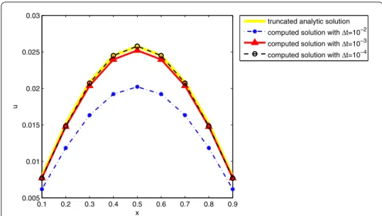
sinc-collocation method solving the arising system solved by the Linsolve package (SMLP) and the sinc-collocation method solving the arising system by the Tikhonov regularization (SMTR) witht= –_,_t_{= }–_{, and}_t_{= }–_{. In Figure  and Figure , we can also}

observe that the computational solution is highly consistent with the truncated analytical solution whentis selected small enough. Furthermore, in Table , the maximum point-wise errors and condition numbers for various values ofNatt= .,t= –_{, and}_T_{= }

for SMLP and SMTR are reported, which shows the improved rate of convergence when the number of sinc points increases. Also, the global maximum pointwise errors atN=  andt= –_{are plotted in Figure (a) for SMLP and in Figure (b) for SMTR in order}

to compare with the thin plate spline-radial basis function method (TPS-RBF), inverse multiquadric-radial basis function method (IMQ-RBF), and hyperbolic secant-radial ba-sis function method (Sech-RBF) (see []) witht= –_at_N_{= . These ﬁgures show}

that our method achieved more accurate results with less data grid points. Convergence curves of Table  are plotted in Figure . This ﬁgure indicates that the maximum errors decline at an exponential rate with respect to N for both SMLP and SMTR, and these graphs conﬁrm the theoretical results.

Example  Consider the following nonhomogenous Volterra partial integro-diﬀerential equation [, ]:

ut(x,t) =

t



(t–s)–/uxx(x,s)ds+f(x,t),  <x< ,  <t< ,

u(,t) =u(,t) = , ≤t≤,

u(x, ) =sin(πx), ≤x≤.

In the case of

f(x,t) = t

/ √

π

(15)

(16)

Figure 1 Truncated analytic and computed solutions of Example 1 withN= 4 att= 1 by using the Linsolve package.

Figure 2 Truncated analytic and computed solutions of Example 1 withN= 4 att= 1 by using

Tikhonov regularization.

Table 2 Results for Example 1 att= 0.01

N SMLP SMTR Cond(P) =PP–1

4 1.10×10–2 _8.27_×₁₀–3 _4.61_×₁₀2

8 2.85×10–3 _7.94_×₁₀–4 _6.71_×₁₀3

16 4.68×10–4 9.32×10–5 3.88×104 32 9.75×10–5 4.71×10–5 1.30×105

the analytic solution is given byu(x,t) =sinπx– _t√/

π sinπx. We apply our presented

(17)

Figure 3 The global maximum pointwise errors atN= 4 andt= 10–3(a) by using the Linsolve package, (b) by using of Tikhonov regularization.

Figure 4 Convergence of the SMLP and SMTR methods for various values ofNatt= 0.01,t= 10–4_,

andT= 1.

Table 3 Results for Example 2

n t = 10–5 t = 10–6

QWM SMLP SMTR QWM SMLP SMTR

50 4.9343e–004 5.1621e–005 7.5561e–006 1.5630e–005 9.8142e–006 2.7356e–006 150 2.5228e–003 2.9006e–004 8.6902e–005 8.0470e–005 9.8142e–006 2.9441e–006 250 5.3616e–003 6.4177e–004 1.1924e–004 1.7272e–004 2.0303e–005 9.1242e–006 350 8.7631e–003 1.0796e–003 6.6327e–004 2.8572e–004 3.4165e–005 1.5836e–005 450 1.2588e–002 1.5898e–003 1.1745e–004 4.1611e–004 5.0328e–005 2.3042e–005

in the solutions have been computed for th, th, th, th, and th time levels and tabulated in Table , which shows that the sinc method in comparison with QWM is considerably accurate. The analytic and exact solutions are compared in Figure  for

(18)

Figure 5 Analytic and computed solutions of Example 2 witht= 10–6_and_N_{= 32 by using the} Linsolve package.

Figure 6 The global maximum pointwise errors atN= 32 andt= 10–6(a) by using the Linsolve

package, (b) by using Tikhonov regularization.

Figure 7 The global maximum pointwise errors forN= 32 att= 0.00045,t= 10–6, andT= 1 (a) by

using the SMLP method, (b) by using the SMTR method.

Example  Consider equation () in the nonhomogenous form whenk(t–s) = (π(t–

(19)

solu-Table 4 Results for Example 3

N t = 10–5 t = 10–6 t = 10–7

SMLP SMTR SMLP SMTR SMLP SMTR

8 2.75×10–3 _8.52_×₁₀–4 _1.05_×₁₀–3 _8.28_×₁₀–4 _3.57_×₁₀–6 _9.81_×₁₀–7

2.83×10–3 _8.94_×₁₀–4 _2.58_×₁₀–3 _8.41_×₁₀–4 _1.65_×₁₀–4 _7.34_×₁₀–6

2.87×10–3 _9.86_×₁₀–4 _2.61_×₁₀–3 _9.73_×₁₀–4 _4.35_×₁₀–4 _6.52_×₁₀–5

2.88×10–3 _9.71_×₁₀–3 _2.61_×₁₀–3 _8.84_×₁₀–3 _6.13_×₁₀–4 _1.41_×₁₀–4

16 2.75×10–4 _7.32_×₁₀–5 _2.63_×₁₀–4 _7.28_×₁₀–5 _9.00_×₁₀–5 _6.87_×₁₀–7

2.92×10–4 _6.54_×₁₀–5 _2.66_×₁₀–4 _1.79_×₁₀–5 _2.56_×₁₀–4 _5.62_×₁₀–6

6.45×10–4 _8.30_×₁₀–5 _2.67_×₁₀–4 _5.48_×₁₀–5 _2.61_×₁₀–4 _6.42_×₁₀–6

1.08×10–3 9.24×10–5 2.67×10–4 6.74×10–5 2.61×10–4 7.83×10–6

32 5.28×10–5 9.12×10–6 9.81×10–6 5.41×10–6 8.66×10–6 1.19×10–7 2.92×10–4 4.37×10–5 9.81×10–6 4.09×10–6 8.66×10–6 4.72×10–7 6.45_×10–4 _5.83_×₁₀–5 _2.04_×₁₀–5 _6.49_×₁₀–6 _8.66_×₁₀–6 _7.28_×₁₀–7

1.08_×10–3 _7.34_×₁₀–5 _3.43_×₁₀–5 _8.51_×₁₀–6 _8.66_×₁₀–6 _8.63_×₁₀–7

64 5.28×10–5 _3.41_×₁₀–6 _1.67_×₁₀–6 _9.86_×₁₀–7 _6.11_×₁₀–8 _7.53_×₁₀–8

2.92×10–4 _1.92_×₁₀–5 _9.24_×₁₀–6 _5.17_×₁₀–6 _2.28_×₁₀–7 _8.91_×₁₀–8

6.45×10–4 _4.56_×₁₀–5 _2.04_×₁₀–5 _6.84_×₁₀–6 _6.45_×₁₀–7 _9.52_×₁₀–8

1.08×10–3 _5.37_×₁₀–5 _3.43_×₁₀–5 _7.13_×₁₀–6 _9.44_×₁₀–7 _1.54_×₁₀–7

Figure 8 Truncated analytic and computed solutions of Example 3 witht= 0.00001 andN= 16 by

using the Linsolve package.

tion is given by []

u(x,t) =

_∞

k=

(–)k(π

_t/₎k

( + k)

+t ∞

k=

(–)k (π

_t/₎k

( + k)

sin(πx).

To evaluate the analytic solution practically at a specific point, the infinite series given above is truncated by the termk= . In Table , we show the results of the th, th, th, and th time levels of the three different grid sizest= –_,_t_{= }–_{, and}

t= –_{for SMLP and SMTR methods when}_N_{= , , , , which verify that the sinc}

(20)

Figure 9 The global maximum pointwise errors atN= 16 andt= 10–5_{(a) by using the Linsolve} package, (b) by using Tikhonov regularization.

Figure 10 The global maximum pointwise errors forN= 16 att= 0.0035,t= 10–5_{, and}_T_{= 1 (a) by}

using the Linsolve package, (b) by using Tikhonov regularization.

6 Conclusions

In this paper, the sinc-collocation method was applied to solve linear Volterra partial integro-differential equations by using the Linsolve package and Tikhonov regularization methods for a final ill-conditioned system. To illustrate the effectiveness of the method, some examples were solved based on the proposed algorithm. Also, the convergence of the method was given. The results show that the proposed method is practically reliable and consistent in comparison with other mentioned methods, and using the Tikhonov regularization method for solving the final ill-conditioned algebraic system, the rate of convergence improved.

Acknowledgements

The authors would like to thank the reviewers for their constructive comments to improve the quality of this work.

Competing interests

The authors declare that they have no competing interests.

Authors’ contributions

(21)

Author details

1_{Department of Mathematics, Central Tehran Branch, Islamic Azad University, Simaye Iran Street, Tehran, 14676-86831,}

Iran.2_{School of Mathematics, Iran University of Science and Technology, Daneshgah Street, Tehran, 16846-13114, Iran.} 3_{Department of Mathematics, Shahid Chamran University of Ahvaz, Golestan Blvd, Ahvaz, 61357-83151, Iran.}

Publisher’s Note

Springer Nature remains neutral with regard to jurisdictional claims in published maps and institutional aﬃliations.

Received: 10 July 2017 Accepted: 31 October 2017

References

1. McLean, W, Mustapha, K: A second-order accurate numerical method for a fractional wave equation. Numer. Math.

105(3), 481-510 (2007)

2. McLean, W, Thomée, V, Wahlbin, LB: Discretization with variable time steps of an evolution equation with a positive-type memory term. J. Comput. Appl. Math.69(1), 49-69 (1996)

3. McLean, W, Thomée, V: Numerical solution of an evolution equation with a positive-type memory term. ANZIAM J.

35(1), 23-70 (1993)

4. Schneider, W, Wyss, W: Fractional diﬀusion and wave equations. J. Math. Phys.30(1), 134-144 (1989) 5. Renardy, M, Nohel, JA: Mathematical Problems in Viscoelasticity, vol. 35. Longman, Harlow (1987)

6. Yanik, EG, Fairweather, G: Finite element methods for parabolic and hyperbolic partial integro-diﬀerential equations. Nonlinear Anal., Theory Methods Appl.12(8), 785-809 (1988)

7. Fakhar-Izadi, F, Dehghan, M: An eﬃcient pseudo-spectral Legendre-Galerkin method for solving a nonlinear partial integro-diﬀerential equation arising in population dynamics. Math. Methods Appl. Sci.36(12), 1485-1511 (2013) 8. Avazzadeh, Z, Rizi, ZB, Ghaini, FM, Loghmani, G: A numerical solution of nonlinear parabolic-type Volterra partial

integro-diﬀerential equations using radial basis functions. Eng. Anal. Bound. Elem.36(5), 881-893 (2012) 9. Fakhar-Izadi, F, Dehghan, M: Space-time spectral method for a weakly singular parabolic partial integro-diﬀerential

equation on irregular domains. Comput. Math. Appl.67(10), 1884-1904 (2014)

10. Mustapha, K, McLean, W: Discontinuous Galerkin method for an evolution equation with a memory term of positive type. Math. Comput.78(268), 1975-1995 (2009)

11. Dehghan, M: Solution of a partial integro-diﬀerential equation arising from viscoelasticity. Int. J. Comput. Math.83(1), 123-129 (2006)

12. Tang, J, Xu, D: The global behavior of ﬁnite diﬀerence-spatial spectral collocation methods for a partial

integro-differential equation with a weakly singular kernel. Numer. Math., Theory Methods Appl.6(3), 556-570 (2013) 13. Luo, M, Xu, D, Li, L: A compact difference scheme for a partial integro-differential equation with a weakly singular

kernel. Appl. Math. Model.39(2), 947-954 (2015)

14. Kim, CH, Choi, UJ: Spectral collocation methods for a partial integro-diﬀerential equation with a weakly singular kernel. ANZIAM J.39(3), 408-430 (1998)

15. Bialecki, B, Fairweather, G: Orthogonal spline collocation methods for partial diﬀerential equations. J. Comput. Appl. Math.128(1), 55-82 (2001)

16. Yoon, J-M, Xie, S, Hrynkiv, V: Two numerical algorithms for solving a partial integro-diﬀerential equation with a weakly singular kernel. Appl. Appl. Math.7(1), 133-141 (2012)

17. Biazar, J, Asadi, MA: FD-RBF for partial integro-diﬀerential equations with a weakly singular kernel. Appl. Comput. Math.4(6), 445-451 (2015)

18. Long, W, Xu, D, Zeng, X: Quasi wavelet based numerical method for a class of partial integro-diﬀerential equation. Appl. Math. Comput.218(24), 11842-11850 (2012)

19. Linz, P: Analytical and Numerical Methods for Volterra Equations. SIAM, Philadelphia (1985)

20. Rashidinia, J, Zarebnia, M: Solution of a Volterra integral equation by the sinc-collocation method. J. Comput. Appl. Math.206(2), 801-813 (2007)

21. Rashidinia, J, Maleknejad, K, Taheri, N: Sinc-Galerkin method for numerical solution of the Bratu’s problems. Numer. Algorithms62(1), 1-11 (2013)

22. Rashidinia, J, Barati, A, Nabati, M: Application of sinc-Galerkin method to singularly perturbed parabolic convection-diﬀusion problems. Numer. Algorithms66(3), 643-662 (2014)

23. Rashidinia, J, Barati, A: Numerical solutions of one-dimensional non-linear parabolic equations using sinc collocation method. Ain Shams Eng. J.6(1), 381-389 (2015)

24. El-Gamel, M: A note on solving the fourth-order parabolic equation by the sinc-Galerkin method. Calcolo52(3), 327-342 (2015)

25. Maleknejad, K, Khalilsaraye, IN, Alizadeh, M: On the solution of the integro-diﬀerential equation with an integral boundary condition. Numer. Algorithms65(2), 355-374 (2014)

26. Sugihara, M: Near optimality of the sinc approximation. Math. Comput.72(242), 767-786 (2003) 27. Lund, J, Bowers, KL: Sinc Methods for Quadrature and Diﬀerential Equations. SIAM, Philadelphia (1992) 28. Stenger, F: Numerical Methods Based on Sinc and Analytic Functions, vol. 20, p. 565. Springer, New York (2012) 29. Dixon, J: On the order of the error in discretization methods for weakly singular second kind non-smooth solutions.

BIT Numer. Math.25(4), 623-634 (1985)

30. Marshall, AW, Olkin, I, Arnold, B: Inequalities: Theory of Majorization and Its Applications. Springer, London (2010) 31. Hansen, PC: Rank-Deﬁcient and Discrete Ill-Posed Problems: Numerical Aspects of Linear Inverse p. 128. SIAM,

Philadelphia (1998)

32. Tang, T: A finite difference scheme for partial integro-differential equations with a weakly singular kernel. Appl. Numer. Math.11(4), 309-319 (1993)