Alternate control delayed systems

(1)

R E S E A R C H

Open Access

Alternate control delayed systems

Yuming Feng

1,2

_{, Dan Tu}

3

_{, Chuandong Li}

1*

_{and Tingwen Huang}

4

*_{Correspondence: [email protected]} 1_{School of Electronic Information}

Engineering, Southwest University, Chongqing, 400715, P.R. China Full list of author information is available at the end of the article

Abstract

In the previous paper (Fenget al.in Adv. Differ. Equ. 2014:305, 2014), we have already used sandwich control to control a system. But when we considered the influence of delay, can sandwich control also be applied in the delayed system? In order to answer this question, we first introduce the alternate delayed system, then we study the exponential stability of delayed chaotic neural networks by means of alternate control. Some sufficient conditions are given in terms of a set of linear matrix inequalities to ensure the exponential stability of the system. Numerical simulations are presented to verify the correction of the obtained results.

Keywords: alternate control delayed system; globally exponential stabilization; Lu oscillator

1 Introduction

Alternate control [] is a special case of switching control [] and is a generalization of in-termittent control [, ]. In an alternate control system, two diﬀerent controls are applied alternately. So there is notrest timefor the control. This system is suitable for the case in which the time is precious.

In [] Fenget al.studied the alternate control system without delay. They have obtained some conditions in terms of LIMs to ensure the stability of the non-delayed system. For delayed systems [–], we know that the methods used are diﬀerent from the ones without delay. There are many papers about delayed system [–]. A delayed system is much more diﬃcult to study than the non-delayed one, we are trying to get some conditions to ensure the stability of the delayed system in the theory of control [–].

In this paper, we consider the inﬂuence of the delay of the system by means of alternate control, that is to say, we study the delayed system by means of alternate control. First of all, we introduce an alternate delayed system. Then we investigate the stability of it by constructing a Lyapunov function, and we obtain stability conditions in terms of LMIs. Lastly we study the stability of Lu oscillator by using the results obtained in the paper.

2 Problem formulation and preliminaries

Consider a class of delayed nonlinear systems described by

˙

x(t) =Ax(t) +f(x(t)) +g(x(t–τ)) +u(t), t> ,

x(t) =φ(t), t∈[–τ, ], ()

wherex∈Rn_{presents state vector,}_f _and_g_{are continuous nonlinear functions of}_Rn_→_Rn

withf() =g() =  and there exist two diagonal matricesL =diag(l(),l ()  , . . . ,l

() n )≥

(2)

andL=diag(l() ,l

For stabilizing the origin of system () by means of periodically alternate control, we assume that the control imposed on the system is of the following form:

u(t) =

It is obvious that system () is a classical switched system where the switching rule only depends on the time. Speciﬁcally, the switching rule of system () depends onTandθ.

In the sequel, we will use the following deﬁnitions and lemmas.

Lemma (Sanchez and Perez []) Given any real matrices,, of appropriate

(3)

Lemma (Halany inequality []) Assume thatτ > andω: [μ–τ,∞)→[,∞)is a continuous function such that

˙

ω(t)≤–aω(t) +b sup

t–τ≤θ≤t ω(θ)

is satisﬁed for all t≥μ.If a>b> ,then

ω(t)≤ω(μ)exp–γ(t–μ), t≥μ,

whereω(t) =sup_t–_τ_≤_θ_≤_tω(θ)andγ> is the smallest real root of the equation

a–bexp(γ τ) =γ.

Lemma ([]) Assume thatτ> andω: [μ–τ,∞)→[,∞)is a continuous function such that

˙

ω(t)≤aω(t) +bω(t–τ)

is satisﬁed for all t≥μ.If a> and b> ,then

ω(t)≤ω(μ)expη(t–μ+τ), t≥μ,

whereω(t) =sup_t–_τ_≤θ≤_tω(θ)andη> is the unique root of the equation

a+bexp(–ητ) =η.

Throughout this paper, we usePT_,_λ

M(P) andλm(P) to denote the transpose, the

maxi-mum eigenvalue and the minimaxi-mum eigenvalue of a square matrixP, respectively.xis used to denote the Euclidean norm of the vectorx. The matrix norm · is also re-ferred to as the Euclidean norm. We useP>  (< ,≤,≥) to denote a symmetrical positive (negative, semi-negative, semi-positive) deﬁnite matrixP.f(x(t–_)) is deﬁned by

f(x(t–

)) =limt→t– f(x(t)).

3 Main results

Theorem  Ifθ>τ and there exist a symmetric and positive deﬁnite matrix P∈Rn×n_, positive scalar constants g> ,g> ,q> ,q> ,> ,> ,η> andη> such that the following hold:

() PA+ATP+PK+KTP+ (+η)P+–L+gP≤,

() PA+AT_P₊_PK

+KTP+ (+η)P+– L–gP≤,

() η_–L–qP≤,

() η–_ L–qP≤,

() g>qandγ(θ–τ) –η(T–θ+τ) > ,

(4)

exponentially stable,and

Proof Let us construct the following Lyapunov function:

(5)

which implies that

Vx(t)≤Vx(mT+θ)expη(t–mT–θ+τ), () whereη>  is the unique root of the equationg+qexp(–ητ) =η.

It follows from () and () that () If  <t≤θ, then we have that

Vx(t)≤Vx()exp(–γt). So

Vx(θ)= sup

θ–τ≤t≤θ

V(t)≤ sup

θ–τ≤t≤θ

Vx()exp(–γt)=Vx()exp–γ(θ–τ).

() Ifθ<t≤T, then we have that

Vx(t)≤Vx(θ)expη(t–θ+τ)

≤Vx()exp–γ(θ–τ) +η(t–θ+τ).

So

Vx(T)≤Vx()exp–γ(θ–τ) +η(T–θ+τ). () IfT<t≤T+θ, then we have that

Vx(t)≤Vx(T)exp–γ(t–T)

≤Vx()exp–γ(t–T) –γ(θ–τ) +η(T–θ+τ).

So

Vx(T+θ)≤Vx()exp–γ(θ– τ) +η(T–θ+τ). () IfT+θ<t≤T, then we have that

Vx(t)≤Vx(T+θ)expη(t–T–θ+τ)

≤Vx()expη(t–T–θ+τ) –γ(θ– τ) +η(T–θ+τ).

So

Vx(T)≤Vx()expη(T–θ+τ) – γ(θ–τ). () If T<t≤T+θ, then we have that

Vx(t)≤Vx(T)exp–γ(t– T)

(6)

So

V(x(T+θ)≤Vx()expη(T–θ+τ) – γ(θ–τ).

() If T+θ<t≤T, then we have that

Vx(t)≤Vx(T+θ)expη(t– T–θ+τ)

≤Vx()expη(t– T–θ+τ) + η(T–θ+τ) – γ(θ–τ).

So

Vx(T)≤Vx()expη(T–θ+τ) – γ(θ–τ).

By induction, we have that

() IfmT<t≤mT+θ,i.e., t–_Tθ<m≤_Tt, then we have that

Vx(t)≤Vx()exp–γt–m(T–θ+τ)+mη(T–θ+τ). ()

() IfmT+θ<t≤(m+ )T,i.e., _Tt <m+ ≤t+T–_T θ, then we have that

Vx(t)≤Vx()expη(t–mT–θ+τ) +mη(T–θ+τ) – (m+ )γ(θ–τ)

=Vx()exp–γ(m+ )(θ–τ) +ηt– (m+ )(θ–τ). ()

From () we know that

Vx(t)≤Vx()exp–γt–m(T–θ+τ)+mη(T–θ+τ)

≤Vx()exp–γmT–m(T–θ+τ)+mη(T–θ+τ) =Vx()exp–γ(θ–τ) –η(T–θ+τ)m

<Vx()exp

–γ(θ–τ) –η(T–θ+τ)t–θ

T

, ()

wheremT<t≤mT+τ. From () we know that

Vx(t)≤Vx()exp–γ(m+ )(θ–τ) +ηt– (m+ )(θ–τ)

≤Vx()exp–γ(m+ )(θ–τ) +η(m+ )T– (m+ )(θ–τ) =Vx()exp–γ(θ–τ) –η(T–θ+τ)(m+ )

<Vx()exp

–γ(θ–τ) –η(T–θ+τ)t

T

≤Vx()exp

–γ(θ–τ) –η(T–θ+τ)t–θ

T

, ()

(7)

It follows from () and () that, for anyt> ,

From Lemma , we know that the two conditions of Theorem  are equivalent to the following two LMIs, respectively:

Proof In fact, the previous four conditions can imply

(8)

and

Thus, the ﬁfth condition of Theorem  is valid. So the proof is completed.

Remark  In order to judge the global exponential stability of system (), Corollary  needs to determine the existence of a symmetric and positive deﬁnite matrixP∈Rn×n

and seven positive scalar constants,,η,η,q,qandηby the four linear matrix

in-equalities listed in it, while Theorem  has to determine the existence of a symmetric and positive deﬁnite matrixP∈Rn×nand eight positive scalar constants,,η,η,q,q,g

andgby the ﬁve conditions of it. From this view of point, Corollary  is more applicative

than Theorem .

4 Numerical example

Consider the neural oscillator model described by the following delayed diﬀerential equa-tion:

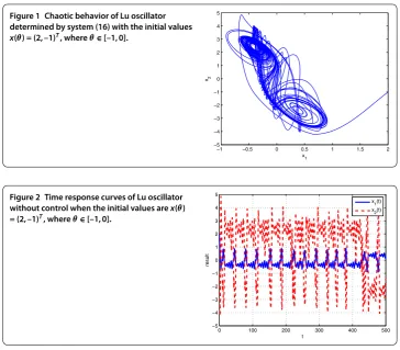
This model was namedLu oscillator[] and it is shown to be chaotic as in Figure . The time response curves are shown in Figure .

It is easy to obtain that

fx(t)  =fTx(t)fx(t)

(9)

Figure 1 Chaotic behavior of Lu oscillator determined by system (16) with the initial values

x(θ) = (2, –1)T, whereθ∈[–1, 0].

Figure 2 Time response curves of Lu oscillator without control when the initial values arex(θ) = (2, –1)T_{, where}_θ_∈_{[–1, 0].}

Choosing

K=diag(–, –), K=diag(–, –),

withT=  andθ= ., solving LMIs (), (),η_–L–qP≤,η– L–qP≤ and

in-equalitiesg>q,γ(θ– ) –η(T–θ+ ) > , whereγ >  is the smallest real root of the

equationg–qexp(γ) =γ andη>  is the unique root of the equationg+qexp(–η) =η,

we obtain a feasible solution:

= ., = ., η= , η= , g= ., g= .,

q= ., q= .,

and

P=

. . . .

.

Thus by Theorem  we obtain that the origin of system () is globally exponentially sta-ble. The time response curves of Lu oscillator with alternate control are shown in Figure , while Figure  shows the corresponding control signal.

(10)

Figure 3 Time response curves of Lu oscillator under alternate control withT= 3,θ= 1.5,K1

= diag(–10, –10),K2= diag(–6, –6) and the initial

valuesx(θ) = (2, –1)T_{, where}_θ_∈_{[–1, 0].}

Figure 4 Control signal for Lu oscillator ofT= 3, θ= 1.5,K1= diag(–10, –10) andK2= diag(–6, –6).

Choosing

K=diag(–, –), K=diag(–, –),

withT=  andθ= ., solving LMIs (), (),η–_ L–qP≤ andη– L–qP≤, where g=γ +qexp(γ τ) andγ =η(T–_θ_–θ_τ+τ)+qandg=η–qexp(–ητ) > , we obtain a feasible

solution:

= ., = ., η= , η= ,

q= ., q= ., η= .

and

P=

. . . .

.

(11)

Figure 5 Time response curves of Lu oscillator under alternate control withT= 3,θ= 1.5,K1

= diag(–15, –15),K2= diag(–11, –11) and the

initial valuesx(θ) = (2, –1)T_{, where}_θ_∈_{[–1, 0].}

Figure 6 Control signal for Lu oscillator ofT= 3, θ= 1.5,K1= diag(–15, –15) andK2= diag(–11,

–11).

5 Conclusions

This paper studies the delayed system by using alternate control method. Some conditions to ensure the stability of the system are given in terms of linear matrix inequalities. By the results obtained, the Lu oscillate is controlled.

Competing interests

The authors declare that they have no competing interests.

Authors’ contributions

The ideal ofalternate control delayed systemwas proposed by CL and YF. The main theory was proved by YF and DT. The paper was typed by YF and TH and all the ﬁgures were provided by TH. All authors read and approved the ﬁnal manuscript.

Author details

1_{School of Electronic Information Engineering, Southwest University, Chongqing, 400715, P.R. China.}2_{School of}

Mathematics and Statistics, Chongqing Three Gorges University, Wanzhou, Chongqing, 404100, P.R. China.3_Department

of Mathematics, Texas A&M University at Qatar, P.O. Box 23874, Doha, Qatar.4_{School of Physical Education, Southwest}

University, Chongqing, 400715, P.R. China.

Acknowledgements

This research is supported by the Natural Science Foundation of China (Grant No: 61374078), NPRP Grant No. NPRP 4-1162-1-181 from the Qatar National Research Fund (a member of Qatar Foundation), Scientiﬁc & Technological Research Foundation of Chongqing Municipal Education Commission (Grant Nos. KJ1401006, KJ1401019) and the Fundamental Research Funds for the Central Universities (Grant No. XDJK2015D004).

Received: 2 December 2014 Accepted: 24 April 2015

References

1. Feng, Y, et al.: Alternate control systems. Adv. Diﬀer. Equ.2014, 305 (2014)

2. Tanwani, A, Shim, H, Liberzon, D: Observability for switched linear systems: characterization and observer design. IEEE Trans. Autom. Control58(4), 891-904 (2013)

(12)

4. Huang, T, Li, C, Liu, X: Synchronization of chaotic systems with delay using intermittent linear state feedback. Chaos

18, 033122 (2008)

5. Xia, W, Cao, J: Pinning synchronization of delayed dynamical networks via periodically intermittent control. Chaos19, 013120 (2009). doi:10.1063/1.3071933

6. Yang, X, Cao, J: Stochastic synchronization of coupled neural networks with intermittent control. Phys. Lett. A373(36), 3259-3272 (2009)

7. Yang, X: Can neural networks with arbitrary delays be ﬁnite-timely synchronized? Neurocomputing143, 275-281 (2014)

8. Zheng, G, Cao, J: Robust synchronization of coupled neural networks with mixed delays and uncertain parameters by intermittent pinning control. Neurocomputing141(2), 153-159 (2014)

9. El’sgol’ts, LE, Norkin, SB: Introduction to the Theory and Application of Diﬀerential Equations with Deviating Arguments. Academic Press, New York (1973)

10. Liao, X, Wang, L, Yu, P: Stability of Dynamical Systems. Monograph Series on Nonlinear Science and Complexity. Elsevier, Amsterdam (2007)

11. Liao, X, Yu, P: Absolute Stability of Nonlinear Control Systems. Springer, New York (2008)

12. Yu, J, Liu, L, Wang, L, Tan, M, Xu, D: Turning control of a multilink biomimetic robotic ﬁsh. IEEE Trans. Robot.24(1), 201-206 (2008)

13. Shen, Y, Xu, D, Tan, M, Yu, J: Mixed visual control method for robots with self-calibrated stereo rig. IEEE Trans. Instrum. Meas.59(2), 470-479 (2010)

14. Dong, D, Petersen, IR: Quantum control theory and applications: a survey. IET Control Theory Appl.4(12), 2651-2671 (2010)

15. Sanchez, EN, Perez, JP: Input-to-state stability (ISS) analysis for dynamic NN. IEEE Trans. Circuits Syst. I, Regul. Pap.

46(11), 1395-1398 (1999)

16. Boyd, S, Ghaoui, L, Feron, EEI, Balakrishnan, V: Linear matrix inequalities in system and control theory. In: Linear Matrix Inequalities in System and Control Theory. SIAM, Philadephia (1994)

17. Horn, R, Johnson, C: Matrix Analysis. Cambridge University Press, Cambridge (1985)

References

1. Feng, Y, et al.: Alternate control systems. Adv. Differ. Equ.2014, 305 (2014)