Effects of patch size and number within a simple model of patchy colloids

Effects of patch size and number within a simple model of patchy colloids

Achille Giacometti,1,a兲 Fred Lado,2,b兲 Julio Largo,3 Giorgio Pastore,4,c兲 and Francesco Sciortino5,d兲

1

Dipartimento di Chimica Fisica, Università Ca’ Foscari Venezia, Calle Larga S. Marta DD2137, Venezia I-30123, Italy

2_{Department of Physics, North Carolina State University, Raleigh, North Carolina 27695-8202, USA} 3_{Departamento de Física Aplicada, Universidad de Cantabria, Avenida de los Castros s/n,}

Santander 39005, Spain

4_{Dipartimento di Fisica dell’ Università di Trieste, and CNR-IOM UOS Democritos, Strada Costiera 11,}

Trieste 34151, Italy

5_{Dipartimento di Fisica and CNR-ISC, Università di Roma La Sapienza, Piazzale A. Moro 2,}

Roma 00185, Italy

共Received 1 February 2010; accepted 6 April 2010; published online 7 May 2010兲

We report on a computer simulation and integral equation study of a simple model of patchy spheres, each of whose surfaces is decorated with two opposite attractive caps, as a function of the fraction␹ of covered attractive surface. The simple model explored—the two-patch Kern–Frenkel model—interpolates between a square-well and a hard-sphere potential on changing the coverage␹. We show that integral equation theory provides quantitative predictions in the entire explored region of temperatures and densities from the square-well limit␹= 1.0 down to␹⬇0.6. For smaller␹, good numerical convergence of the equations is achieved only at temperatures larger than the gas-liquid critical point, where integral equation theory provides a complete description of the angular dependence. These results are contrasted with those for the one-patch case. We investigate the remaining region of coverage via numerical simulation and show how the gas-liquid critical point moves to smaller densities and temperatures on decreasing ␹. Below ␹⬇0.3, crystallization prevents the possibility of observing the evolution of the line of critical points, providing the angular analog of the disappearance of the liquid as an equilibrium phase on decreasing the range for spherical potentials. Finally, we show that the stable ordered phase evolves on decreasing␹from a three-dimensional crystal of interconnected planes to a two-dimensional independent-planes structure to a one-dimensional fluid of chains when the one-bond-per-patch limit is eventually reached. ©2010 American Institute of Physics.关doi:10.1063/1.3415490兴

I. INTRODUCTION

Spherically symmetric potentials have become a well-established paradigm of colloidal science in past decades.1 This is because, at a sufficiently coarse-grained level, colloi-dal surface composition can be regarded as uniform with a good degree of confidence, so that relevant interactions de-pend only on relative distances among the particles. Recent advances in chemical particle synthesis2have however chal-lenged this view by emphasizing the fundamental role of surface colloidal heterogeneities and their detailed chemical compositions. This is particularly true for an important sub-class of colloidal systems, namely, proteins, where the pres-ence of anisotropic interactions cannot be neglected, even at the minimal level.3–5Directional interactions introduce novel properties in such systems. These properties depend both on the number of contacts共i.e., the valency兲and the amplitude of these interactions共i.e., flexibility of the bonds兲, a notable example of this class being hydrogen-bond interactions, ubiquitous in biological, chemical, and physical processes.6,7

As a reasonable compromise between the high complex-ity of interactions governing the above systems and the nec-essary simplicity required for a minimal model, patchy-sphere models stand out for their remarkable success in this rapidly evolving field.8–11See Ref.12for a recent review on the subject.

Within this class of models, interactions are spread over a limited part of the surface, either concentrated over a num-ber of pointlike spots10,13 or distributed over one or more extended regions.14,15 While the former have the consider-able advantage of a simple theoretical scheme,16 which al-lows a first semiquantitative description, the latter can easily account for both the effect of the number of contacts and their amplitude, unlike “spotty” interactions which are al-ways limited by the one-bond-per-site constraint.

In this paper we consider a particular model due to Kern and Frenkel15 of this patchy-spheres class wherein short-range attractive interactions, of the square-well共SW兲 form, are distributed over circular patches on otherwise hard spheres 共HS兲. Interactions between particles 共spheres兲 are then attractive in the SW-SW interfacial geometry or purely hard-sphere repulsive under the HS-SW or HS-HS interfacial geometries, and can sustain more than one bond—in fact, as many as the geometry allows—even in the case of a single

a兲_{Electronic mail: [email protected].}

b兲_{Electronic mail: [email protected].}

c兲_{Electronic mail: [email protected].}

d兲_{Electronic mail: [email protected].}

patch assigned to each sphere. A number of real systems ranging from surfactants to globular proteins can be de-scribed with simplified interactions of these particular forms, with well-defined solvophilic and solvophobic regions, and despite their simplicity patchy hard spheres have already shown a remarkable richness of theoretical predictions.5,14,15,17–19Notwithstanding the discontinuous na-ture of the angular interactions, highly simplified integral equation approaches are possible,17 but only very recently has a complete well-defined scheme, within the framework of the reference hypernetted-chain 共RHNC兲 integral equa-tion, been proposed and solved for patchy spheres.20 This integral equation belongs to a class of approximate closures which have been extensively exploited in the field of mo-lecular associating fluids.21 Its main advantage over other available approximations共other than its less-accurate parent HNC closure兲 lies in the fact that it relies on a single ap-proximation, for the bridge function appearing in the exact relation between pair potential and pair distribution function g共12兲,21,22 to directly yield structural and thermodynamic properties that include the Helmholtz free energy and the chemical potential with no further approximations.23,24In ad-dition, it can be made to display enhanced consistency among different thermodynamic routes.25 This is an impor-tant point when analyzing fluid-fluid phase diagrams such as we propose to do here. We thus build on our previous work with the one-patch potential20 to study the two-patch case and its relationship with its one-patch counterpart. In addi-tion to RHNC integral equaaddi-tion results, we provide dedicated Monte Carlo simulations which can assess the performance of RHNC. We find that RHNC provides a robust representa-tion of both structural and thermophysical properties of the two-patch Kern–Frenkel model for a wide range of coverage ␹共the ratio between attractive and total hard-sphere surface兲, extending from an isotropic SW to a bare HS potential. The competition arising between phase separation and polymer-ization is discussed in terms of the angular dependence of the pair correlation function and the structure factor. Finally, a comparison between the one-patch and two-patch phase dia-grams shows a strong impact on the different morphology and stable structures obtained in the two cases.

We also report numerical simulation results of the model in the region where the RHNC integral equations do not numerically converge, to explore the low temperature, small ␹ limit. We find that for ␹⬍0.3 it becomes impossible to investigate the low-temperature disordered phases, since the system quickly transforms into an ordered structure, which itself depends on the coverage value. Indeed, on decreasing␹ one progressively enters the region where the maximum number of contacts per patch evolves from four to two and eventually reaches the one-bond-per-patch condition. When three or four bonds per patch are possible, the observed or-dered structure is a crystal of interconnected planes, while when only two contacts are possible, particles order them-selves into a set of disconnected planes.

The patchy interaction model examined here can be re-garded as a prototype of a special colloidal architecture where there exist competitive interactions on the colloidal surface that drive, by free energy minimization, the different

colloidal particles through a spontaneous self-assembly pro-cess into complex superstructures whose final target can be experimentally probed and properly tuned.26The possibility, discussed in the present study, of identifying the position of the gas-liquid coexisting lines and its relative interplay with different structures opens up fascinating scenarios in material science on the possibility of novel material design exploiting a bottom-up process not requiring human intervention.

II. THE TWO-PATCH KERN–FRENKEL MODEL

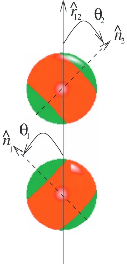
As a paradigmatic model for highly anisotropic interac-tions, we take the Kern–Frenkel15 two-patch model where two attractive patches are symmetrically arranged as polar caps on a hard sphere of diameter ␴. Each patch can be reckoned as the intersection of a spherical shell with a cone of semiamplitude ␪0 and vertex at the center of the sphere.

Consider spheres 1 and 2 and letrˆ₁₂ be the direction joining the two sphere centers, pointing from sphere 1 to sphere 2

共see Fig.1兲. The orientation of spherei is defined by a unit vectornˆi⬅nˆ_i共t兲passing outward through the center of one of its patches, to be arbitrarily designated as the “top”共t兲patch. The patch on the opposite, “bottom”共b兲 pole is then identi-fied with the outward normalnˆ_i共b兲= −nˆi.

Two spheres attract via a square-well potential of range

␭␴ and depth ⑀ if any combination of the two patches on each sphere are within a solid angle defined by ␪0and

oth-erwise repel each other as hard spheres. The pair potential then reads15

n

^

θ

n

^

1

θ

12

r^

FIG. 1. The two-patch Kern–Frenkel potential. Each sphere is divided into an attractive part共color code: green兲and a repulsive part共color code: red兲. The attractive part is positioned on two symmetrically distributed patches identified by unit vectorsnˆ_i共t兲_=nˆ

iandnˆi

共b兲_{= −nˆ}

i共i= 1 , 2兲, where the

orienta-tion vectorsnˆ1,nˆ2define angles␪1,␪2with the vectorrˆ12joining the centers

⌽共12兲=␾共r12兲⌿共nˆ₁,nˆ₂,rˆ12兲, 共1兲

where

␾共r兲=

冦

⬁, 0⬍r⬍␴ −⑀, ␴⬍r⬍ ␭␴

0, ␭␴⬍r

冧

共2兲

and

⌿共nˆ₁,nˆ₂,rˆ12兲

=

冦

1, if nˆ₁共p1兲·rˆ₁₂ⱖcos␪₀ and −nˆ₂共p2兲·rˆ₁₂ⱖcos␪₀

0, otherwise

冧

, 共3兲

wherep1,p2=torb indicates which patch, top or bottom, is

involved on each sphere. The unit vectorsnˆi共␻i兲are defined by the spherical angles ␻i=共␪i,␸i兲 in an arbitrarily oriented

coordinate frame and rˆ12共⍀兲 is identified by the spherical angle ⍀ in the same frame. Reduced units, temperature Tⴱ =kBT/⑀, and density␳ⴱ=␳␴3will be used throughout.

This model was introduced by Kern and Frenkel,15 pat-terned after a similar model studied by Chapmanet al.,14 as a minimal model where both the distributions and the sizes of attractive surface regions on particles can be tuned. In this sense, the model constitutes a useful paradigm lying between spherically symmetric models which do not capture the specificity of surface groups, not even at the simplest pos-sible level, and models with highly localized interactions having the single-bond, single-site limitation.10,13,27 Several previous studies have already examined potentials of the Kern–Frenkel form using numerical simulations,5,15 corresponding-state arguments,18 highly simplified integral equation theories,17 and pertubation theories.19 More recently,20the single patch Kern–Frenkel potential was stud-ied using a more sophisticated integral equation approach based on the RHNC approximation coupled with rather pre-cise and extensive Monte Carlo simulations. In the present paper, we extend this last study to the two-patch Kern– Frenkel potential and provide new methodologies specific for the angular distribution analysis.

We define the coverage ␹ as the fraction of the total sphere surface covered by attractive patches. Thus␹= 1 cor-responds to a fully symmetric square-well potential while ␹= 0 corresponds to a hard-sphere interaction and the model smoothly interpolates between these two extremes in the in-termediate cases 0⬍␹⬍1. The two-patch potential is ex-pected to present qualitative as well as quantitative differ-ences with respect to its one-patch counterpart. One interesting question, for instance, concerns the subtle inter-play between distribution and size of the attractive patches on the fluid-fluid phase separation diagram. It is now well established5,15,17,20 that as coverage decreases the fluid-fluid coexistence line progressively diminishes in width and height. Indeed, this feature can be exploited to suppress phase separation altogether to enhance the possibility of studying glassy behavior10,13 and cannot be accounted for with a simple temperature and density rescaling,17 although corresponding-state type of arguments can be proposed.18On

the other hand, the above mechanism can significantly de-pend on how the same reduced attractive region is distributed on the surface of particles. In Ref. 17, for instance, it was suggested that lines of decreasing critical temperature as a function of decreasing coverage, for the one-patch and two-patch Kern–Frenkel models with very short-range interac-tions, could cross each other at a specific coverage: for low coverages, critical temperatures for the one-patch model lie above the two-patch counterpart whereas the opposite is true for larger coverages. This would have far-reaching conse-quences on the phase diagram, as phase separation would occur at higher or lower temperatures for fixed coverage, depending on the specific allotment of the coverage. Another interesting issue regards miscellization phenomena, present in the one-patch version of the model,28which is expected to be replaced by polymerization共or chaining兲in the two-patch version.29

III. INTEGRAL EQUATION WITH RHNC CLOSURE AND MONTE CARLO SIMULATIONS

The Ornstein–Zernike equation22 defines the direct cor-relation functionc共12兲in terms of the pair correlation func-tion h共12兲=g共12兲− 1; it is convenient for computation to write it using the indirect correlation function␥共12兲=h共12兲 −c共12兲 instead ofh共12兲. We have then

␥共12兲= ␳

4␲

冕

A second, or “closure,” equation coupling␥共12兲andc共12兲is needed. The general form for this is22

c共12兲= exp关−␤⌽共12兲+␥共12兲+B共12兲兴− 1 −␥共12兲, 共5兲

where ␤=共kBT兲−1 and a third pair function, the so-called

“bridge” function B共12兲, has also been introduced. While known in a formal sense as a power series in density,22B共12兲 cannot in fact be evaluated exactly and at this point an ap-proximation is unavoidable. The RHNC apap-proximation re-places the unknownB共12兲with a known versionB0共12兲from some “reference” system. In practice, only the hard-sphere model is today well-enough known to play the role of refer-ence system. Here we will use the Verlet–Weis–Henderson– Grundke parametrization30,31forB0共12兲=BHS共r12;␴0兲, where

␴0 is the reference hard-sphere diameter. Some

computa-tional details of the RHNC integral equation approach can be found in Ref.20共see Appendix A兲, so only the most relevant equations will be repeated here.

Solution of the Ornstein–Zernike integral equation for molecular fluids21seemingly requires expansions in spherical harmonics of the angular dependence of all pair functions, a need that would be very problematic in the case of the dis-continuous angular dependence in the present⌽共12兲. In fact, the integral equation algorithm allows ⌽共12兲 to remain unexpanded.20 There is a potential problem however in evaluating the Gauss–Legendre quadratures used in the nu-merical solution, in that of the angles␪1,␪2, . . . ,␪nused for

an nth-order quadrature, none is likely to coincide with the angle ␪0 defining the semiamplitude of a patch. Thus the

prob-lem is ameliorated in the followingad hocfashion.

From the interaction⌽共12兲of Eq.共3兲, the total coverage ␹ can be computed in terms of␪0as

␹2₌ 1

共4␲兲2

冕

+⌰共− cos␪₁− cos␪0兲⌰共− cos␪₂− cos␪0兲

+⌰共− cos␪1− cos␪0兲⌰共cos␪2− cos␪0兲兴, 共6兲

where ⌰共x兲 is the Heaviside step function, equal to 1 if x

⬎0 and 0 ifx⬍0. The integrals can be readily evaluated to give15

␹= 2 sin2␪0

2. 共7兲

This quantity can also be numerically evaluated by Gauss– Legendre quadrature using the n roots ␪j of the Legendre

polynomial Pn共cos␪兲 and the computed result compared with the exact value共7兲. We may then vary n so as to find that numbern共typically kept between 30 and 40兲that mini-mizes the known error in computing␹. All Gaussian quadra-tures for that␹value are then evaluated with the same num-bernof points, thus ensuring that minimal error arises from the selected angular grid.

In an axialrframe21withrˆ₁₂=zˆ, the internal energy per particle in unitskBT is obtained from

␤U

N = − 2␲␳␤⑀

冕

␭␴

drr2具g共r,␻1,␻2兲⌿共␻1,␻2兲典␻₁␻₂, 共8兲

where具¯典_␻=共1/4␲兲兰d␻¯denotes an average over spheri-cal angle ␻ and where we have written out g共12兲 =g共r,␻1,␻2兲. Similarly, the pressurePis computed from the

compressibility factor ␤P

␳ = 1 + 2 3␲␳␴

3_{兵具y共␴,␻}

1,␻2兲e␤⑀⌿共␻1,␻2兲典␻₁␻₂

−␭3具y共␭␴,␻1,␻2兲关e␤⑀⌿共␻1,␻2兲− 1兴典␻1␻2其, 共9兲

where the cavity functiony共12兲=g共12兲e␤⌽共12兲has been intro-duced. The angular integrations in these expressions are evaluated with Gauss–Legendre and Gauss–Chebyshev quadratures. Finally, the dimensionless free energy per par-ticle ␤F/N and chemical potential ␤␮ can also be directly computed from the pair functions produced by the RHNC equation; the overall calculation is optimized by choosing the reference hard sphere diameter␴0so as to minimize the

free energy functional.20We solve the RHNC equations nu-merically onrandkgrids ofNr= 2048 points, with intervals ⌬r= 0.01␴and⌬k=␲/共Nr⌬r兲, using a standard Picard itera-tion method.22 The square-well width is set at ␭= 1.5 as a reasonable value dictated by the availability of isotropic square well results.32Further details of these and other com-putations can be found in Ref.20.

For an assessment of the performance of the RHNC in-tegral equation, we also perform NVT, grand canonical, and Gibbs ensemble Monte Carlo共MC兲simulations33 following the path set in the one-patch case.20Standard NVT MC

simu-lations of a system of 1000 particles are used to compute structural information 共pair correlation functions and struc-ture factors兲for comparison with integral equations results, whereas grand canonical and Gibbs ensemble MC共GEMC兲 are used to locate critical parameters and coexisting phases. The exact locations of the critical points 共points connected by the thick dashed green line in Fig.2兲have been obtained from the MC data assuming the Ising universality class and properly matching the density fluctuations with the known fluctuations of the magnetization close to the Ising critical point.36 For GEMC, we use a system of 1200 particles, which partition themselves into two boxes whose total vol-ume is 4300␴3_{, corresponding to an average density of ␳}ⴱ

= 0.27. At the lowest temperature considered, this corre-sponds to roughly 1050 particles in the liquid box and 150 particles in the gas box共of side⬇13␴兲. On average, the code attempts one volume change every five particle-swap moves and 500 displacement moves. Each displacement move is composed of a simultaneous random translation of the par-ticle center 共uniformly distributed between ⫾0.05␴兲 and a rotation共with an angle uniformly distributed between ⫾0.1 rad兲 around a random axis. We studied systems of size L = 7 up toL= 10 to estimate the size dependence of the critical point, with an average of one insertion/deletion step every 500 displacement steps in the case of grand canonical Monte Carlo 共GCMC兲. We also performed a set of GCMC simula-tions for different choices of T and␮ to evaluate ␳ⴱ共␮,T兲. See Ref.20and additional references therein for details.

IV. NUMERICAL RESULTS

A. Coexistence line

Locating coexistence lines is not an easy task within integral equation theory, given the fact that virtually all inte-gral equations are unable to access the critical region with reliable precision due to significant thermodynamic inconsis-tencies among various possible routes to thermodynamics, a consequence of the approximation buried in the closure Eq.

共5兲. The RHNC closure is no exception to this rule, but has the strong advantage of relying on a single approximation expressed by the choice of the reference bridge function

0 0.1 0.2 0.3 0.4 0.5 0.6 0.7 0.8 0.9

ρ∗ 0

0.2 0.4 0.6 0.8 1 1.2

T

*

χ=1.0 χ=0.9 χ=0.8 χ=0.7 χ=0.6 χ=0.5 χ=0.4 χ=0.3

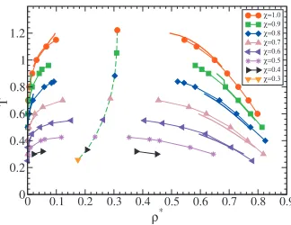
FIG. 2. Fluid-fluid coexistence lines of the two-patch model for different values of the coverage ranging from a full square-well potential down to

B0共12兲, at odds with other available closures which require additional approximations in constructing various thermody-namic quantities such as the chemical potential. Here we follow the protocol outlined in Ref. 32 for the isotropic square-well potential and Ref. 20 for the one-patch Kern– Frenkel potential, where both the well-known pseudosolu-tions shortcoming37 and the numerical drawbacks38 can be conveniently accounted for.

Figure 2 depicts the location of the fluid-fluid coexist-ence line for the two-patch case upon varying the coverage ␹. The limiting case ␹= 1 corresponds to the square-well potential. Both MC 共points兲 and RHNC 共thick solid lines兲 results are shown. As previously noted, RHNC is not able to approach the critical point close enough to provide a direct estimate of its location. However, since it provides a quite good description of the low-temperature part of the coexist-ence line, we tried to use these data to approximately locate the critical point.

Visual inspection of the RHNC coexistence points re-veals, in the cases where it is possible to go closer to the critical region, an unphysical change in curvature of the co-existence line moving from low to high temperature. For this reason, for each coverage we selected only data clearly con-sistent with a rectilinear diameter law. Then we fitted those data with the following function 共corresponding to the first correction to the scaling兲:39

␳l−␳g=a共Tc−T兲␤共1 +b共Tc−T兲⌬兲, 共10兲

where the values of the exponents␤= 0.325 and⌬= 0.54 are appropriate for the three-dimensional Ising model universal-ity class.40,41 Once Tc and the amplitudes a, b have been

determined, the critical density can be obtained from the rec-tilinear diameter best fit. The numerical results of such a procedure are compared with MC estimates of the critical points in TableI. It is evident that even though in general the validity of Eq. 共10兲 is deemed to be limited to a smaller neighborhood of the critical point;40 in the present case it provides an acceptable procedure for a quick first estimate of the critical point location.

As the coverage decreases, the coexistence line shrinks and moves to lower temperature and density, as expected from an overall-decreasing attractive interaction. This trend can be tracked rather precisely by MC simulations down to remarkably low coverages共␹= 0.3兲and RHNC correctly

re-produces this evolution down to␹= 0.6 coverage. Below this value, more powerful algorithms are required to achieve good numerical convergence.

A few remarks are here in order. The coexistence curves shown in Fig. 2 are consistent with previous analogous re-sults reported in Ref.15but extend the range of temperatures and, more importantly, the range of coverages 共␹ values兲. This allows a quantitative measure of the significant devia-tion from the simple mean-field-like results, which can be obtained from the simple scaling共not shown兲Tⴱ→Tⴱ/␹, as suggested by the second-virial coefficient B2共Tⴱ兲 for this model,15

B2共Tⴱ兲 B₂共HS兲 = 1 −␹

2_共␭3_{− 1兲共e}␤⑀_{− 1兲, 共11兲}

B₂共HS兲 being the hard-sphere result. This is also consistent with the breakdown of the above simple scaling at the level of the third virial coefficient, derived in Ref.17for the com-panion patchy sticky-hard-sphere model. As we shall see later on, the dependence of the critical temperature and den-sity onboththe coverageandthe number of patches is one of the main results of the present work. As a final point, we note that all curves in Fig. 2 collapse into a single master curve upon scalingTⴱ→Tⴱ/T_cⴱ, in agreement with Ref.15.

B. Low-coverage results

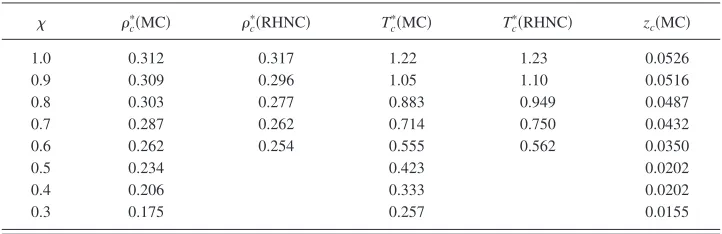
Below ␹= 0.3, it becomes impossible to properly esti-mate the location of the critical point or the density of the coexisting gas and liquid phases. Indeed, the gas-liquid sepa-ration becomes pre-empted by crystallization into a structure that depends on the value of␹. Hence, the liquid phase, as an equilibrium phase, ceases to exist for small ␹. This is strongly reminiscent of the disappearance of the liquid phase using spherical potentials when the range of the interaction becomes smaller than about 10% of the particle diameter,42–44thus providing the angular analog of the same phenomenon. Interestingly enough, the crystal structure which is spontaneously observed during the simulation de-pends on the value of␹, since the␹value controls the maxi-mum number of bonds per patch. In the range of ␹ values such that each patch can be involved in four bonds, the ob-served ordered structure is made by planes exposing the SW parts to their surfaces 关see Fig. 3共d兲兴. Particles in the plane are located on a square lattice and adjacent planes are shifted

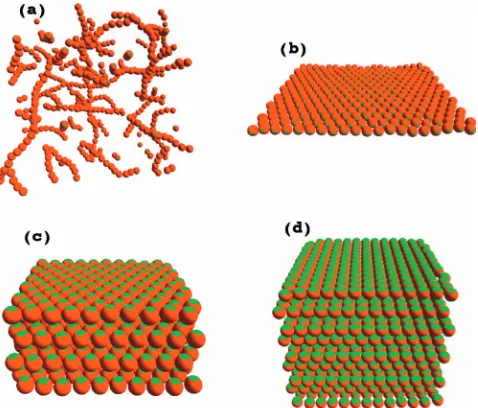
TABLE I. Comparison of the estimated location of critical points from MC and RHNC data共see text兲. In the last columnzc⬅e␤␮is the critical activity.

␹ ␳cⴱ_{共MC兲 ␳c}ⴱ_{共RHNC兲 T}

c

ⴱ_{共MC兲 T}

c

ⴱ_{共RHNC兲 zc共MC兲}

1.0 0.312 0.317 1.22 1.23 0.0526

0.9 0.309 0.296 1.05 1.10 0.0516

0.8 0.303 0.277 0.883 0.949 0.0487

0.7 0.287 0.262 0.714 0.750 0.0432

0.6 0.262 0.254 0.555 0.562 0.0350

0.5 0.234 0.423 0.0202

0.4 0.206 0.333 0.0202

in each direction by a half lattice constant, resulting in a reduced energy of⫺4 per particle共i.e., eight bonded neigh-bors兲. On decreasing ␹ below ␹⬇0.118, the region where only three bonds per particle are possible 共关

冑

冑

struc-ture is made by interconnected planes of particles arranged in a triangular lattice 关see Fig. 3共c兲兴. For 关

冑

冑

pos-sible and the system organizes into independent planes关see Fig.3共b兲兴, this time turning a HS surface to their neighboring planes. Particles in the plane are now arranged on a triangu-lar lattice and each patch is able to bind only to two different neighbors located in the same plane, resulting in a reduced energy per particle of⫺2. When sin␪0becomes smaller than

the value 关2共1 +⌬/␴兲兴−1 共corresponding to ␹⬇0.0572兲, the one-bond-per-patch condition is reached and the system can form only isolated chains 关see Fig. 3共a兲兴. In this limit, the system is expected to behave as the two single-bond-per-patch model.29

C. Structural information

We turn our attention next to structural information, where the advantages of a reliable integral equation approach become evident. One has to keep in mind that Gibbs en-semble and GCMC simulations are particularly painstaking, due to the combined effect of the required low temperatures

and the aggregation properties of the fluid 共as detailed be-low兲, so that many of the state points examined here require several weeks of computer time. On the other hand, the RHNC integral equation, while rather demanding from an algorithmic point of view共see, e.g., Appendix A of Ref.20兲 is a rapidly convergent scheme yielding solutions on the or-der of minutes, depending on the temperatures consior-dered. A more profound advantage stems from the fact that, within the approximation defined by the RHNC closure, all possible pair structural information is in fact exactly available, unlike MC calculations where, though available in principle, their statistics would be so limited as to make such calculations impractical. Thus, only the pair correlation function g共12兲 averaged over angle rˆ12共⍀兲 is computed. By symmetry, the resulting pair function in this context depends only on r

⬅r12 and cos␪12⬅nˆ1·nˆ2 and will be denoted here as

g

¯共r, cos␪12兲; see Appendix B in Ref.20for details.

Consider then the unaveraged pair correlation function g共12兲=g共r,␻1,␻2兲 from RHNC in an axial frame with rˆ12

=zˆ. Two noteworthy configurations occur when 共a兲 all four patches lie along the same line关we denote this as the parallel

共储兲 configuration, with nˆ₁·nˆ₂=⫾1, the actual labeling of each patch being unimportant兴 and when 共b兲 patches on sphere 2 lie on an axis perpendicular to those of sphere 1关in this casenˆ₁·nˆ₂= 0, which we denote as the crossed共X兲 con-figuration兴.

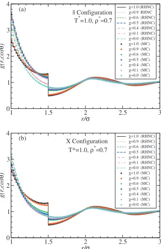
Figure4reports the results for the case ␭= 1.5,␳ⴱ= 0.7, and Tⴱ= 1.0, which has been selected so that the fluid is above the coexistence line for all considered coverages, with configurations储and X in the top and bottom panels

respec-FIG. 3. Representation of the structures observed at small coverages␹.共a兲 The case of coverages such that each patch can be involved in only one interaction. In this case, the system forms polydisperse chains. The snapshot here refers to the case␳ⴱ= 0.01 andTⴱ= 0.07.共b兲Values of␹such that each patch can be involved in only two interactions. In this case, at lowTthe system forms bonded planes interacting with each other only via excluded volume interactions. The snapshot shows one such plane.共c兲Values of␹ such that each patch can be involved in only three interactions. The crystal is now formed by interconnected planes, with a triangular arrangement of the particles in the plane. Adjacent planes are shifted in such a way that each particle sits in correspondence to the center of a triangle of the previous and following planes.共d兲Values of␹such that each patch can be involved in at most four interactions. The crystal is now formed by interconnected planes, with a square arrangement of the particles in the plane. Adjacent planes are shifted in such a way that each particle sits in correspondence to the center of a square of the previous and following planes.

1 1.5 2 2.5 3

r/σ 0

2 4 6 8

g(12)

χ=1.0 χ=0.9 χ=0.8 χ=0.7 χ=0.6 χ=0.5 χ=0.4 χ=0.3 χ=0.2 χ=0.1 χ=0.0 T*=1.0,ρ∗=0.70 || Configuration

(a)

χ=1.0

χ=0.9 χ=0.8 χ=0.7 χ=0.6 χ=0.5 χ=0.4 χ=0.3 χ=0.2 χ=0.1

χ=0.0

1 1.5 2 2.5 3

r/σ 0

1 2 3 4

g(12)

χ=1.0 χ=0.9 χ=0.8 χ=0.7 χ=0.6 χ=0.5 χ=0.4 χ=0.3 χ=0.2 χ=0.1 χ=0.0 T*=1.0,ρ∗=0.70

X Configuration (b)

χ=1.0

χ=0.9 χ=0.8 χ=0.7 χ=0.6

χ=0.5 χ=0.4 χ=0.3 χ=0.2χ=0.1 χ=0.0

FIG. 4. Behavior ofg共12兲from the RHNC equation for different coverages and two specific orientations of the patches:储configuration corresponding to

nˆ1·nˆ2=⫾1 共a兲 and X configuration corresponding to nˆ1·nˆ2= 0 共b兲. All

curves are for a state point with ␭= 1.5,␳ⴱ= 0.7, andTⴱ= 1.0. Black and green lines show the limiting cases of square-well共␹= 1兲and hard-sphere

tively. Values of coverages range from a full square-well po-tential共␹= 1兲to a hard-sphere potential共␹= 0兲.

As coverage decreases, the contact valuer=␴+ of the储

configuration has the unusual behavior of first a slight in-crease from␹= 1 to␹= 0.5, followed by a more marked in-crease starting at ␹= 0.4 up to the very small coverage ␹ = 0.1 limit which eventually backtracks to roughly the same value as at ␹= 0.4 in the hard-sphere limit. At the opposite side of the well,r=共␭␴兲−_{, an even more erratic behavior is}

observed, with an increase in the range 0.7⬍␹⬍1, then a decrease for 0.3⬍␹⬍0.6, a new increase down to ␹= 0.1, and a final sudden decrease to the hard sphere value␹= 0. A somewhat similar feature occurs in the X configuration where within the entire well region ␴+ⱕrⱕ共␭␴兲− one ob-serves a sudden decrease from ␹= 1 to ␹= 0.9 and a more gradual increase until reaching the highest value for the HS case. It is worth noting that in the X configuration there is no discontinuous jump atr=␭␴for any value␹⬍1. The reason for this has already been addressed in Ref. 20for the one-patch case. Outside the first shell, there is a very weak de-pendence on the coverage, with a slight shift in the location of the second peak from a value of r⬇2.25␴ at the SW ␹ = 1 to a value ofr⬇1.8␴ for lower␹.

We compare RHNC integral equation results with MC simulations in Fig.5. As noted above, only the averaged pair function¯g共r, cos␪12兲can be compared and this is done in the figure for different values of the coverage␹at the same state point共Tⴱ= 1.0, ␳ⴱ= 0.7兲and for the same 储 and X configu-rations considered earlier. The good overall performance of RHNC in representing MC results is apparent as both contact values at the well edges and the jump discontinuities are very

well reproduced. It is instructive to contrast these results with those of Fig. 4, as many of the abrupt changes appear-ing in the actual pair correlation function are smoothed out by the orientational average carried out here. For instance, the characteristic jump at r=␭␴ of the 储 configuration共top panel兲 progressively decreases as coverage is reduced and disappears in the hard-sphere limit. Conversely, the jump is present also in the X configuration共bottom panel兲unlike the corresponding case of the fullg共12兲. In addition, the strong increase in the 储 configuration for low coverages is not present in this figure; as remarked earlier, this level of detail ing共12兲 is one of the main advantages of an integral equa-tion approach.

An additional useful quantity to consider, in view of its direct experimental access through scattering experiments,22 is the structure factor, which will be denoted S000共k兲 within our theoretical framework.20,21,23 This is also strongly re-lated, via Hankel transforms, to the radial distribution func-tiong000共r兲, which isg共12兲averaged over all orientations␻1

and␻2of the patches and of the relative angular position⍀.

Note thatg000共r兲is also the simplest rotational invariant共see Ref. 21and Appendix B兲.

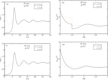
The structure factor and the radial distribution function are reported in Fig.6for two representative values of cover-age,␹= 0.8 and␹= 0.2, corresponding to almost fully attrac-tive and almost fully repulsive limits. These values have been selected at the same state point previously considered

共Tⴱ= 1.0, ␳ⴱ= 0.7兲as having a very different behavior within the first shell␴ⱕrⱕ␭␴. This high-density result is also con-trasted with a low-density state point ␳ⴱ= 0.1 at the same temperature, a value which, in the temperature-density plane, lies symmetrically with respect to the coexistence curves in the single fluid phase for all coverages共see Fig.2兲.

A few features are worth noting. For density ␳ⴱ= 0.7 there is a significant coverage dependence, where the contact valueg000共␴+_{兲for␹= 0.2 coverage is larger than that for the}

corresponding␹= 0.8 case and, conversely, the jump present at the other extreme␭␴−is much smaller in the former than in the latter case. A similar feature also occurs for the low-density state point␳ⴱ= 0.1. This results from an angular av-erage of the results given in Fig. 4. Likewise, there is a marked difference in the behavior of the structure factor S000共k兲 for the high-density case␳ⴱ= 0.7, both in the height of the first peak 关related to the g000共␴+_{兲 value兴 and of the}

secondary peaks 关related to the behaviors of g000共r兲 in the ␴⬍r⬍␭␴region and of theg000共␭␴⫾兲discontinuity兴. Simi-larly, in the low-density branch ␳ⴱ= 0.1, the large S000共0兲 value for the␹= 0.8 coverage case is signaling the approach to a spinodal instability which is clearly not present in the corresponding␹= 0.2 coverage.

One natural interpretation of the above results is the pro-gressive rearrangement of the distribution within the first shell upon varying both the coverage and the density. To support this view, we consider the angular distribution within the first shell in the next subsection.

D. Angular distribution

The nonmonotonic dependence ofg共12兲in terms of the distancer/␴for decreasing coverage␹, as illustrated in Fig.

1 1.5 2 2.5 3

r/σ

0 1 2 3 4

g(r,cos

θ

)

χ=1.0(RHNC) χ=0.9RHNC χ=0.6(RHNC) χ=0.5(RHNC) χ=0.4(RHNC) χ=0.1(RHNC) χ=0.0(RHNC) χ=1.0(MC) χ=0.9(MC) χ=0.6(MC) χ=0.5(MC) χ=0.4(MC) χ=0.1(MC) χ=0.0(MC)

|| Configuration

T*=1.0,ρ∗=0.7

(a)

1 1.5 2 2.5 3

r/σ

0 1 2 3 4

g(r,cos

θ

)

χ=1.0(RHNC) χ=0.9(RHNC) χ=0.6(RHNC) χ=0.5(RHNC) χ=0.4(RHNC) χ=0.1(RHNC) χ=0.0(RHNC) χ=1.0(MC) χ=0.9(MC) χ=0.6(MC) χ=0.5(MC) χ=0.4(MC) χ=0.1(MC) χ=0.0(MC)

X Configuration

T*=1.0,ρ∗=0.7

(b)

FIG. 5. Behavior of the averaged¯g共r, cos␪兲for different coverages and two specific orientations of the patches:储configuration corresponding tonˆ₁·nˆ₂

4, is rather intriguing and requires an explanation. A similar, albeit different, feature occurs even in the one-patch case, as shown in Ref.20. We tackled this in two ways, illustrated in the following.

All previous representations ofg共12兲have been depicted in the molecular axial frame, where nˆ₁·rˆ₁₂= 1, so that patches on sphere 1 are parallel to the vector r12 joining

sphere 1 with sphere 2. This is clearly preventing an under-standing of the angular distribution of the patches around a given sphere 1, that is, as a function ofrˆ12共⍀兲.

This is however a needless restriction, as one can start from the expression forg共12兲in a general共laboratory兲frame and study the dependence on the angle ⍀ for fixed patch directions nˆ₁ and nˆ₂. In Figs.4–6, we notice that the main dependence on coverage␹ stems from the region within the well,␴ⱕrⱕ␭␴; it suffices therefore to investigate the aver-age⍀ dependence by integrating over the radial variabler within this region. We further note that there is azimuthal symmetry with respect to the␸variable, so that we can focus on the␪dependence. The details of the analysis are reported in Appendix A, where it is shown that the relevant quantity is g

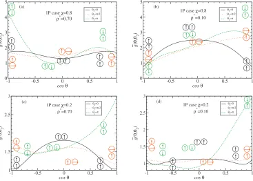
¯共␪,␪2兲, which is a function of the angle␪共polar dependence ofrˆ12共⍀兲兲and of the polar angle␪₂of the patches on particle 2, given that the patches on particle 1 lie along thezˆaxis. We report comparative calculations for both low 共␳ⴱ= 0.1兲 and high共␳ⴱ= 0.7兲density at identical temperatureTⴱ= 1.0 at two representative coverages,␹= 0.8, representing a case with al-most all attraction, and␹= 0.2, as representative of an almost hard-sphere case. These are the same conditions considered in Fig.6; the results are reported in Fig.7. Let us consider first the high-density,␳ⴱ= 0.7, situation as depicted in the two left panels for ␹= 0.8 共a兲 and ␹= 0.2 共c兲. Here, the ␹= 0.8

case yields a very well-defined pattern with a periodically modulated distribution of the patches in symmetrical fashion as indicated by the trimodal distribution as a function of the relative positional angle ␪, so that 0 ,␲/2 ,␲ are almost equally represented. 共Note that ␪= 0 ,␲ are necessarily equivalent due to the up-down symmetry of the two-patch distribution.兲The two interstitial minima are a consequence of the reduced valency—the corresponding fully symmetri-cal result under this condition would be a flat distribution around the value 1.66 in between the two maxima and minima—so this slightly favors perpendicular orientation of the patches along the forward 共or backward兲 direction and parallel orientation along the transversal direction. Under low coverage共␹= 0.2兲conditions, on the other hand, there is clear evidence of a parallel orientation of the patches along the forward共or backward兲direction, the opposite being true for a perpendicular orientation of the patches. This confirms the tendency to filament formations previously alluded to. The situation is even more evident at low density,␳ⴱ= 0.1, as shown in the right two panels共b兲and共d兲.

E. Coefficients of rotational invariants

Additional insights on the angular correlations of patch distributions can be obtained by considering other coeffi-cients hl1l2l共_r兲_=gl1l2l共_r兲₋␦

l₁l₂l,000 of the rotational invariants

␺l1l2l共_r兲_{as defined in Eqs.}共_A1兲_and共_A2兲_{; they have proven}

to be of invaluable help in discriminating between parallel and antiparallel configurations occurring in different models such as dipolar hard spheres45,46 and Heisenberg spin fluids.47 Some relevant properties of these coefficients are also listed in Appendix B, where we display explicit expres-sions for the first few coefficients.

0 5 10 15 20 25 30

kσ

0 0.5 1 1.5 2 2.5

S000

(k)

ρ* =0.70

ρ* =0.10 χ=0.8

2P case (a)

1 1.5 2 2.5 3

r/σ

0 1 2 3 4

g000

(r)

ρ*_=0.70

ρ* =0.10 χ=0.8

2P case (b)

0 5 10 15 20 25 30

kσ

0 0.5 1 1.5 2 2.5

S000

(k)

ρ* =0.70

ρ* =0.10 χ=0.2

2P case (c)

1 1.5 2 2.5 3

r/σ

0 1 2 3 4

g000

(r)

ρ*_=0.70

ρ*_=0.10

χ=0.2 2P case (d)

FIG. 6. Behavior of the structure factorS000共k兲 关共a兲 and共c兲兴 and the radial distribution functiong000共r兲 关共b兲and 共d兲兴 for coverages␹= 0.8 and␹= 0.2,

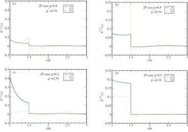
In the two-patch case, we note that all coefficients with l₁orl₂odd vanish, so we depict the first nonvanishing coef-ficientsh220_共r兲,h222_共r兲,h022_共r兲=h202_{共r兲in Fig.8for the same}

state points as before. Note that the leftmost two curves,共a兲 and共c兲, correspond to density␳ⴱ= 0.7, temperature Tⴱ= 1.0, coverages ␹= 0.8共a兲 and␹= 0.2共c兲, and are plotted on the

same scale. While qualitative trends are similar, the two cases have significantly different behavior. Within a given coverageh220_共r兲andh222_{共r兲are almost coincident, with}

posi-tive correlation in the well region␴⬍r⬍␭r, whereash022_共r兲

has decreasing positive correlation in the same region and negative correlation for r⬎␭␴. Numerical values, on the

-1 -0.5 0 0.5 1

cosθ

0 1 2 3 4 5

g(

θ,θ

2

)

θ2=0,π

θ2=π/2

ρ∗=0.70

2P caseχ=0.8

(a)

-1 -0.5 0 0.5 1

cosθ

1 1.5 2 2.5 3

g(

θ,θ

2

)

θ2=0,π

θ₂=π/2

ρ∗=0.70

2P caseχ=0.2

(c)

-1 -0.5 0 0.5 1

cosθ

0 1 2 3 4 5

g(

θ,θ

2

)

θ2=0,π

θ2=π/2

ρ*

=0.10 2P caseχ=0.8 (b)

-1 -0.5 0 0.5 1

cosθ

1 1.5 2 2.5 3

g(

θ,θ

2

)

θ2=0,π

θ₂=π/2

ρ*

=0.10

2P caseχ=0.2

(d)

FIG. 7. Angular distributions¯g共␪,␪2兲as functions of cos␪for two different orientations of the patches on sphere 2, given that sphere 1 is fixed with patches

along thezˆaxis. Results are reported for two different coverages,␹= 0.8关共a兲and共b兲兴and␹= 0.2关共c兲and共d兲兴, and two different densities,␳ⴱ= 0.7关共a兲and

共c兲兴and ␳ⴱ= 0.1关共b兲and共d兲兴, at the same temperatureTⴱ= 1.0. Again, the square-well width was set to␭= 1.5. The colored arrows are cartoons of the orientations of sphere 2 patches, corresponding to␪2= 0,␲/2. Note that these are the same state points considered in Fig.6.

1 1.5 2 2.5 3

r/σ

-0.1 0 0.1 0.2 0.3 0.4 0.5

h

l1 l2 l (r)

220 022 222

ρ*

=0.70 2P caseχ=0.8 (a)

1 1.5 2 2.5 3

r/σ -0.05

0 0.05 0.1 0.15 0.2 0.25

h

l1 l2 l (r)

220 022 222

ρ*

=0.10 2P caseχ=0.8 (b)

1 1.5 2 2.5 3

r/σ

-0.1 0 0.1 0.2 0.3 0.4 0.5

h

l1 l2 l (r)

220 022 222

ρ*

=0.70 2P caseχ=0.2 (c)

1 1.5 2 2.5 3

r/σ -0.05

0 0.05 0.1 0.15 0.2 0.25

h

l1 l2 l (r)

220 022 222

ρ*

=0.10 2P caseχ=0.2 (d)

other hand, differ among each other, with small values for h220共r兲andh222共r兲in the high coverage case␹= 0.8 and sig-nificantly higher values in the low coverage limit␹= 0.2.

Likewise, for the low-density state point ␳ⴱ= 0.1, Tⴱ = 1.0, right-hand-side plots共b兲and共d兲can be unambiguously discriminated between high 共b兲 and low 共d兲 coverages. We shall return to this point in the comparison with the one-patch results, where the physical meaning of these coeffi-cients will be discussed.

V. COMPARISON WITH ONE-PATCH RESULTS

A. Phase diagram

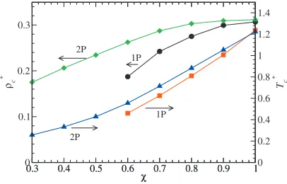
Figure 9 shows the critical parameters for the case of particles with one and two patches, both reported as a func-tion of the total coverage. Here only MC results are reported in view of their precision and reliability. The␹= 1 limit cor-responds to the SW case and coincides for both models. An analogous figure, for the case of adhesive patchy spheres共the limit of the present model for vanishing ranges兲, has been reported in Ref. 17 within a simplified integral equation scheme.

With respect to the adhesive limit, the range of cover-ages which can be explored numerically is significantly wider共for both one-patch and two-patch cases兲. In the case of two patches, crystallization pre-empts the possibility of exploring the smaller values. In the one-patch case, the

pro-cess of micelle formation, also observed experimentally,49 suppresses the phase-separation process28at small ␹values. The critical parameters decrease on decreasing ␹ for both one-patch and two-patch models. The behavior of Tc

can be explained on the basis of a progressive reduction in the attractive surface. The decrease in the critical density becomes significantly pronounced only for the smallest ␹ values and can be attributed to the lower local density re-quested for extensive bonding. Such behavior is analogous to the suppression of the critical density observed when the particle valence decreases.10,50 In the ␹ region where it is possible to evaluate the critical parameters,Tcand␳cfor the

two-patch case are always larger than the corresponding one-patch values, a trend which can be tentatively rationalized on the basis of the ability to form a larger number of contacts and higher local bonded densities for the case in which both poles of the particles can interact attractively with their neighbors. No evidence of a crossing between the two geom-etries is observed. Such a crossing has been predicted by a theoretical approach based on a virial expansion up to third order in density and appropriate closures of the direct corre-lation function.17

It is worth emphasizing that the above dependence on the number of patches, at a given coverage, provides clear evidence of the impossibility of rationalizing the change in the critical line on the basis of a trivial decrease in the at-tractive strength of interactions due to the reduction in cov-erage, as alluded to in Sec. IV A.

For the sake of completeness, we also report RHNC in-tegral equation results for the most relevant thermodynamic quantities, as a function of the coverage␹. These are shown in Table II for the same high-density state, ␳ⴱ= 0.7 at Tⴱ = 1.0, considered above for structural information. Here we present the reduced internal energy per particle and the re-duced excess free energy per particle, U/N⑀ and ␤Fex/N,

respectively, the reduced chemical potential ␤␮, the com-pressibility factor ␤P/␳, and the inverse compressibility ␤共⳵P/⳵␳兲T. These results may be compared with those of Table IV in Ref. 20listing the same quantities for the one-patch counterpart.共We ignore the tiny difference in densities between the two calculated states.兲 The last two columns

0.3 0.4 0.5 0.6 0.7 0.8 0.9 1

χ

0 0.2 0.4 0.6 0.8 1 1.2 1.4

Tc

*

0.3 0.4 0.5 0.6 0.7 0.8 0.9 1

χ

0 0.1 0.2 0.3

ρc

*

2P

2P

1P

1P

FIG. 9. Comparison between the critical parameters observed for the one-patch case共from Ref.48兲and the two-patch case共this work兲.

TABLE II. Values of reduced internal and excess free energies, chemical potential, pressure, and inverse compressibility as a function of the coverage ␹for a fixed state point,␳ⴱ= 0.7, andTⴱ= 1.0. The last two columns report the reference HS diameter␴₀共in units of␴兲and the average coordination number¯z. Expected errors are in the last digits.

␹ U/N⑀ ␤Fex/N ␤␮ ␤P/␳ ␤共⳵P/⳵␳兲T ␴0/␴ ¯z

1.0 ⫺5.46 ⫺2.56 ⫺3.28 0.64 10.33 1.031 10.92

0.9 ⫺4.88 ⫺1.81 ⫺1.79 1.37 11.26 1.026 9.76

0.8 ⫺4.10 ⫺0.98 ⫺0.10 2.24 12.39 1.020 8.20

0.7 ⫺3.25 ⫺0.19 1.53 3.08 13.54 1.014 6.50

0.6 ⫺2.49 0.49 2.88 3.75 14.48 1.010 5.00

0.5 ⫺1.88 1.05 3.94 4.25 15.21 1.007 3.76

0.4 ⫺1.26 1.61 5.00 4.74 15.95 1.005 2.51

0.3 ⫺0.80 2.00 5.75 5.10 16.51 1.003 1.60

0.2 ⫺0.39 2.33 6.39 5.42 17.00 1.001 0.79

0.1 ⫺0.11 2.54 6.79 5.62 17.31 1.000 0.23

give the reference HS diameter␴0stemming from the

varia-tional RHNC scheme共see Ref.20for details兲and the aver-age coordination number within the wells¯z, whose one-patch counterparts are included in Tables IV and V of Ref. 20, respectively. Note that¯zhere is systematically larger than in the one-patch case, in qualitative agreement with the MC results of Fig.9.

B. Angular distribution and coefficients of rotational invariants

Within the RHNC integral approach, the analysis of the angular distribution of patches within the first shell given in Sec. IV D revealed that the cylindrical symmetry of a pair of patches共2P case兲on each particle was very effective in driv-ing the system to morphologically different configurations in the low共20%兲and high共80%兲coverage limits, as illustrated in Fig.7. It is natural to expect a very different situation in the single-patch case 共1P case兲. This is indeed the case as further elaborated below.

For the single patch with␹= 0.2 coverage关Fig.10, bot-tom panels 共c兲 and 共d兲兴 parallel patches 共␪₂= 0兲 are more likely in the perpendicular direction 共␪⬇␲/2 or cos␪⬇0兲, whereas antiparallel patches 共␪₂=␲兲 are more likely in the forward direction 共cos␪⬇1兲. The case of perpendicular patches共␪2=␲/2兲is conversely more or less equally

distrib-uted along the whole angular region 0ⱕ␪ⱕ␲. There is no qualitative difference between the situation of high 共␳ⴱ = 0.7兲 and low共␳ⴱ= 0.1兲 densities as shown by the contrast between the bottom left共c兲and right共d兲panels. Note that the result significantly contrasts with the corresponding results of the two-patches case depicted in Fig.7. Consider now the

opposite situation of very large coverage 共␹= 0.8兲 关Fig. 10共a兲兴where there is a single well-defined peak for antipar-allel orientations 共␪₂=␲兲 in the backward direction 共cos␪

⬇−1兲. Again, this markedly differs from the two-patch case

关Fig. 7, top left panel 共a兲兴, where there is a triple peak for aligned patches共␪2= 0 ,␲兲in the forward共cos␪⬇1兲,

perpen-dicular 共cos␪⬇0兲, and backward 共cos␪⬇−1兲 orientations. This is a dense state point. Under diluted conditions, ␳ⴱ = 0.1, we find a qualitatively similar behavior as in the dense case, with antiparallel alignment in the forward direction

共which cannot be physically distinguished from the back-ward one兲. Clearly the predominant antiparallel alignment is reflecting the tendency to miscellization rather than polymer-ization which is built into the single patch symmetry.

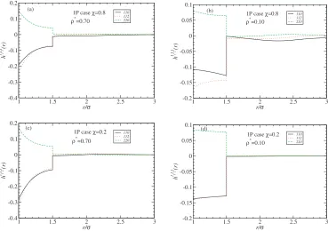
It is also interesting to contrast the coefficients of rota-tional invariants for the one-patch case with those obtained in the two-patch counterpart in Fig. 7. At variance with the two-patch case, here all coefficients are nonvanishing so that we consider the first nonvanishing instances, that is h110共r兲, h112共r兲, and h220共r兲, which are particularly useful as giving the projections over the important invariants.45

We evaluated these coefficients for the same state points considered in the two-patch case in Fig.11for both dense or diluted conditions and small or large coverages. In contrast with the two-patch case, here the effect of coverage appears to be less significant, as can be inferred by inspection of the dense case ␳ⴱ= 0.7 关left panels 共a兲 and共c兲兴. For theh110共r兲 case, the projection coefficient along the ferroelectric invari-ant ⌬共12兲 in Appendix B, we find a negative correlation within the well both for ␹= 0.8 关top left panel 共a兲兴 and ␹ = 0.8关bottom left panel 共c兲兴, as expected from the tendency to form antiparallel alignments. Likewise, the projection

-1 -0.5 0 0.5 1

cosθ

0 1 2 3 4 5

g(

θ,θ

2

)

θ2=0

θ2=π/2

θ2=π

ρ∗=0.70

1P caseχ=0.8

(a)

-1 -0.5 0 0.5 1

cosθ

1 1.5 2 2.5 3

g(

θ,θ2

)

θ₂=0 θ2=π/2

θ2=π

ρ∗=0.70

1P caseχ=0.2 (c)

-1 -0.5 0 0.5 1

cosθ

0 1 2 3 4 5

g(

θ,θ

2

)

θ2=0

θ2=π/2

θ2=π

ρ* =0.10 1P caseχ=0.8

(b)

-1 -0.5 0 0.5 1

cosθ

1 1.5 2 2.5 3

g(

θ,θ2

)

θ₂=0 θ2=π/2

θ2=π

ρ*

=0.10 1P caseχ=0.2

(d)

FIG. 10. Angular distribution¯g共␪,␪2兲for the one-patch model as a function of cos␪for three different orientations of the patch on sphere 2, given that sphere

1 is fixed with patch along thezˆaxis. This is the one-patch counterpart of Fig.7. Results are reported for two different coverages,␹= 0.8关共a兲and共b兲兴and

h112共r兲 along the dipolar invariantD共nˆ₁,nˆ₂,rˆ12兲 is found to be negative and numerically similar toh110共r兲at both cover-ages, again indicating negative correlation to dipolar align-ment. The only positive correlation is found for the h220共r兲 component, which does not distinguish between up and down symmetry, in qualitative agreement with the two-patch analog.

This situation is replicated in the diluted case关right two panels 共b兲and共d兲兴with different numerical values, thus in-dicating that these correlations are signatures of robust ori-entational trends induced by the particular one-side symme-try of the single-patch potential.

VI. CONCLUSIONS AND OUTLOOK

We performed a detailed study of a fluid whose particles interact via a two-patch Kern–Frenkel potential that at-tributes a negative square-well energy whenever any two patches on the spheres are within a solid angle associated with a predefined coverage and within a given distance given by the well width, and a simple hard-sphere repulsion other-wise. This model can be reckoned as a paradigm of a unit system with incompatible elements 共e.g., hydrophobic and hydrophilic兲 that can self-assemble into different complex superstructures depending on the parameters of the original unit共e.g., coverage兲. We exploited state-of-the-art numerical simulations 共standard Metropolis, Gibbs ensemble, and GCMC兲 coupled with RHNC integral equation theory fol-lowing the approach outlined in previous work on a single patch.20On comparing RHNC integral equation with numeri-cal simulations, we find the former to be quantitatively pre-dictive in a large region of coverage, even close to the gas-liquid transition critical region, over a range of coverage

which is significantly larger than the single patch counter-part. The reason for this is attributed to the fact that RHNC uses the approximated hard-sphere bridge function, which retains spherical information, as a unique approximation throughout the entire calculation, a feature which works bet-ter for the more symmetric two-patch case than the highly asymmetric one-patch Kern–Frenkel potential.

Having assessed the reliability of the RHNC integral-equation approach, we fully exploited its capabilities in pro-viding detailed angular information that is typically inacces-sible to MC simulations, as already discussed in Ref. 20. This has been done in two ways. First, by computing the orientational distribution probability of parallel and perpen-dicular alignment of patches within a spherical shell in the region ␴⬍r⬍␭␴. This methodology is able to account for the erratic coverage dependence of the pair correlation func-tiong共12兲by clearly discriminating between small and large coverages at all densities. The same approach also enlightens the characteristic symmetries of the patch distributions when the two-patch case result is contrasted with the one-patch analog. Second, by computing the rotational-invariant coef-ficients that are the projections of g共12兲 over rotational in-variants. Again, this can discriminate between small and large coverages 共at all densities兲 and single and double patches.

Our Monte Carlo results extend those originally obtained by Kern and Frenkel15 for the two-patch case and can be contrasted with those of the corresponding single-patch counterpart20 and those obtained when the radial part of the potential is of the Baxter type.17The RHNC calculation pre-sented here, along with the corresponding calculation carried out in our previous paper,20 together constitute the first

at-1 1.5 2 2.5 3

r/σ -0.4

-0.3 -0.2 -0.1 0 0.1 0.2

h

l1 l2 l (r)

110 112 220

ρ*

=0.70 1P caseχ=0.8

(a)

1 1.5 2 2.5 3

r/σ -0.4

-0.3 -0.2 -0.1 0 0.1 0.2

h

l1 l2 l (r)

110 112 220

ρ*

=0.70 1P caseχ=0.2

(c)

1 1.5 2 2.5 3

r/σ -0.2

-0.15 -0.1 -0.05 0 0.05 0.1

h

l1 l2 l (r)

110 112 220

ρ*

=0.10 1P caseχ=0.8 (b)

1 1.5 2 2.5 3

r/σ -0.2

-0.15 -0.1 -0.05 0 0.05 0.1

h

l1 l2 l (r)

110 112 220

ρ*

=0.10 1P caseχ=0.2 (d)

tempt to apply a well-defined integral equation theory to such highly anisotropic potentials having sharp angular modulation.

An important outcome of our calculations is the clarifi-cation of the combined effect that size and distribution of the patches have on the gas-liquid coexistence lines and critical parameters. The reduction in the bonding surface clearly de-creases the critical temperature, an effect which can be re-lated to the decrease in the bonding energy of the system. More interestingly, it also shows a suppression of the critical density, which can be interpreted along the same lines used in interpreting the valence dependence in patchy colloids.13,50 Indeed, the maximally bonded structures re-quire lower and lower local densities on decreasing␹. Inter-estingly, while in the single-bond-per-patch condition the evolution of the critical parameters on decreasing valence can be followed down to the limit where clustering prevents phase separation,28 in the model studied here crystallization pre-empts the observation of the liquid-gas separation for ␹

⬍0.3. Crystallization is here much more effective due to the analogy between the local fully bonded configuration and the crystal structure. By contrast, crystallization is never ob-served for the one-patch case, where it has been shown that the lowest energy configuration is reached instead via the process of formation of large aggregates 共micelles and vesicles兲or via the formation of lamellar phases.28This dif-ference highlights the important coupling between the orien-tational part of the potential and the possibility of forming extended fully bonded structures. Our results indicate that, for a given coverage, in the two-patch case both the critical temperature and density are slightly higher then their corre-sponding one-patch counterparts, thus indicating that an in-crease in the valence favors the gas-liquid transition, in agreement with previous findings.

A final important consequence of our study concerns the limit of very small coverages that is particularly interesting. Indeed, it is possible to tune the structure of the system and control the topology of its ordered arrangement. By doing this we observed a progression from the case where chains are stable共in the one-bond-per-patch limit兲to the case where independent planes are found, evolving—for slightly larger␹ values—into an ordered three-dimensional crystalline struc-ture. Each of these ordered structures is observed in a re-stricted range of␹ values. This possibility of fine tuning the morphology by controlling the patterning of the particle sur-faces may offer an interesting possibility for specific self-assembling structures.

An additional perspective of our work should be stressed. Several studies 共see, e.g., Ref. 51 and references therein兲exploited spherically symmetric potentials to mimic effective protein-protein interactions, especially in connec-tion with protein crystallizaconnec-tion.52 This is clearly unrealistic for the majority of proteins where the distribution of hydro-phobic surface groups is significantly irregular, a feature that can be captured, at the simplest level of description, by the model studied here. The specific location of the coexistence lines, such as those considered in the present study, have important consequences in the study of pathogenic events for sickle cell anemia53and other human diseases.54

ACKNOWLEDGMENTS

We thank Philip J. Camp and Enrique Lomba for useful suggestions. F.S. acknowledges support from NoE SoftComp Grant Nos. NMP3-CT-2004-502235, ERC–226207– PATCHYCOLLOIDS, and ITN-COMPLOIDS. A.G. ac-knowledges support from PRIN-COFIN Grant No. 2007B57EAB共2008/2009兲.

APPENDIX A: ANGULAR PROPERTIES OFg_„12_…IN A

GENERAL FRAME

The expansion in spherical harmonicsYlm共␻兲ofg共12兲in an arbitrary space frame reads55

g共12兲= 4␲

兺

l₁,l2=0

⬁

兺

l=兩l₁−l2兩 l₁+l2

g共r;l1l2l兲␺l1l2l共␻1␻2⍀兲, 共A1兲

where we introduced the rotational invariants21

␺l₁l₂l_共␻

1␻2⍀兲=

兺

+l1

兺

m₂=−l2 +l2

C共l1l2l;m1m2m1+m2兲

⫻Yl₁m₁共␻1兲Yl₂m₂共␻2兲Yl,mⴱ ₁+m₂共⍀兲. 共A2兲

Note thatg共r;l1l2l兲coincides withgl1l2l共r兲up to a

normaliza-tion constant共see Appendix B兲.

We are free to set the origin of the coordinate frame at the center of particle 1 and choose its orientation so that zˆ =nˆ₁without loss of generality. We first note that

Yl₁m₁共␪1= 0,␸1兲=

冉

2l1+ 1

4␲

冊

1/2

␦m₁0. 共A3兲

Clearly, the orientation of thexandyaxes is then irrelevant, so we may integrate out the angles␸2and␸; this leads to the

average具g共12兲典_␸

2␸, where we note that 具Yl₂m₂共␪2,␸2兲典␸₂

=共− 1兲m2

冋

4␲

共l2−m2兲! 共l2+m2兲!

册

1/2

⫻Pl₂m₂共cos␪2兲

1 2␲

冕

2␲

d␸₂eim₂␸₂

=

冉

冊

1/2

Pl₂共cos␪2兲␦m₂0, 共A4兲

and similarly for具Y_lm

2

ⴱ _{共␪,␸兲典}

␸. Here thePl0共x兲=Pl共x兲are the

usual Legendre polynomials. We have then from Eqs. 共A1兲 and共A2兲that

具g共12兲典_␸

2␸=

兺

l₁,l2,l

g共r;l1l2l兲

冋

共2l1+ 1兲共2l2+ 1兲共2l+ 1兲

4␲

册

1/2

⫻C共l1l2l;000兲Pl₂共cos␪2兲Pl共cos␪兲. 共A5兲

We are interested in the angular behavior within the well, ␴ⱕrⱕ␭␴, so we finally integrate over the radial variabler and define

g

¯共l₁l₂l兲= 1

共␭− 1兲␴

冕

␭␴