MOHAN, SIBIN. Exploiting Hardware/Software Interactions for Analyzing Embedded Systems. (Under the direction of Associate Professor Frank Mueller).
Embedded systems are often subject to real-time timing constraints. Such systems require determinism to ensure that task deadlines are met. The knowledge of the bounds on worst-case execution times (WCET) of tasks is a critical piece of information required to achieve this objective. One limiting factor in designing real-time systems is the class of processors that may be used. Contemporary processors with their advanced architectural features, such as out-of-order execution, branch prediction, speculation, and prefetching, cannot be statically analyzed to obtain WCETs for tasks as they introduce non-determinism into task execution, which can only be resolved at run-time. Such micro-processors are tuned to reduce average-case execution times at the expense of predictability. Hence, they do not find use in hard real-time systems. On the other hand, static timing analysis derives bounds on WCETs but requires that bounds on loop iterations be known statically, i.e., at compile time. This limits the class of applications that may be analyzed by static timing analysis and, hence, used in a real-time system. Finally, many embedded systems have com-munication and/or synchronization constructs and need to function on a wide spectrum of hardware devices ranging from small microcontrollers to modern multi-core architectures. Hence, any sin-gle analysis technique (be it static or dynamic) will not suffice in gauging the true nature of such systems.
This thesis contributes novel techniques that use combinations of analysis methods and constant interactions between them to tackle complexities in modern embedded systems. To be more specific, this thesis
(I) introduces of a new paradigm that proposes minor enhancements to modern processor architec-tures, which, on interaction with software modules, is able to obtain tight, accurate timing analysis results for modern processors;
(II) it shows how the constraint concerning statically bound loops may be relaxed and applied to make dynamic decisions at run-time to achieve power savings;
(III) it represents the temporal behavior of distributed real-time applications as colored graphs cou-pled with graph reductions/transformations that attempt to capture inherent “meaning” in the appli-cation.
by Sibin Mohan
A dissertation submitted to the Graduate Faculty of North Carolina State University
in partial fullfillment of the requirements for the Degree of
Doctor of Philosophy
Computer Science
Raleigh, North Carolina
2008
APPROVED BY:
Dr. Alex Dean Dr. Purush Iyer
Dr. Frank Mueller Dr. Tao Xie
DEDICATION
BIOGRAPHY
Sibin Mohan was born on March 20, 1979 to Mrs. T. Shobhana and Mr. B. M. C. Kumar in Kozhikode (Kerala, India), but has lived mostly in the lovely city that is Bangalore. He completed his schooling at the Frank Anthony Public School (FAPS), Bangalore. He received his Bachelor of Engineering (B.E.) undergraduate degree in Computer Science and Engineering from PES Institute of Technology which is a part of Bangalore University, India. He then worked at Hewlett-Packard India Software Operations, Bangalore, as a Software Engineer for one year.
ACKNOWLEDGMENTS
This dissertation is the culmination of many years of work, all of which have been ex-tremely rewarding. I have been able to reach this goal largely due to the belief, support and wisdom imparted by many people I have had the honour of interacting with over the years. While I try to acknowledge every single one of them, I realize that being only human, I might miss a few names.
To Dr. Frank Mueller, my advisor, I offer sincere thanks and appreciation for having the patience to shepherd me through the journey that was this Ph.D. As the ancient Chinese proverb states, “a journey of a thousand miles begins with a single step.” I realize that this Ph.D., that first important step, would not have been possible without his insight, advice, critique and support. His counsel on research methodology, teaching, presentation skills, writing skills, etc. have all been instrumental in shaping me as a researcher. His management style, dedication towards research and attention to detail is something that I can only hope to emulate. He has also guided and actively assisted me through the long process of searching for future career opportunities.
Some of the best courses I took during my time at NC State was courtesy of Dr. Matt Stallmann. His courses challenged and excited me at the same time and often made me see the field of Computer Science in a new light. He was also gracious enough to mentor me through the process of navigating my way through my first comprehensive teaching assignment.
Comments and questions raised by Dr. Alex Dean, Dr. Purush Iyer and Dr. Tao Xie helped me focus on important issues and avoid pitfalls during the course of my research. I would like to thank them for being a part of my dissertation committee and guidance provided thus.
Dr. Purush Iyer, Dr. Peng Ning, Dr. Nagiza Samatova and Dr. Tao Xie took time off their busy schedules to examine and provide valuable feedback on my job application materials. I am thankful for their feedback and the knowledge that they imparted during the whole process. I am also grateful to Dr. Becky Rufty for her valuable advice on this and related topics. I would also like to thank Dr. David Whalley and Dr. John Regehr for writing reference letters for me.
I would also like to thank Dr. Eric Rotenberg as many of the ideas in this dissertation would not have come up if not for the deep understanding of computer architecture he instilled in me via his courses. I would also like to thank him for making his architecture simulator and toolset available for use in my research. Aravind Anantaraman and Vimal Reddy were always willing to help me to understand and solve problems related to the simulator framework and for that I am grateful.
moves the great machinery in the background. Dr. David Thuente as the Director of Graduate Programs has been very helpful in directing me through the administrative details that go along with being a student. I would also like to thank the Computer Science staff members, Margery Page, Carol Allen, Ginny King and Susan Peaslee, to name but a few.
Not a day goes by that I don’t remember, or feel grateful towards, Mr. Vijayan. His teach-ings on C++, programming paradigms, operating systems, etc. coupled with quick philosophical insights often drew parallels with slices of real life. I attempt to emulate his remarkable teaching style every time I step in front of a classroom full of students. I would also like to thank Dr. Krishna Rao and Mr. Joye Joseph whose teaching had a profound effect on me.
Johannes Helander took a chance on a graduate student he met at a conference and has been a mentor and friend ever since. That was the start of a great opportunity for me; an opportunity to work on some really exciting research ideas. Conversations with him range over a diversity of topics, from cutting-edge research ideas to varieties of beer, all of which ensures that every time I talk to him I come back having learned something new.
Jaydeep, Nirmit, Yifan, Kaustubh, Kiran, Anita, Harini, Anubhav, Nik, Ravi, Chao, Arun, Vivek, Raghuveer and Heshan have all been great lab-mates over the years. Interactions with them resulted in my learning a great deal and often made me look forward to coming in to work every day. I would also like to thank my various room-mates (Salil, Ajit, Rahul, Ishdeep, Sharath) who have had to put up with me and my cooking over the years!
No person is complete without his friends and I consider myself lucky to have some amazing people as close friends. Nisha, whose thought processes resemble mine in uncanny ways, provides a mirror to the inner workings of my mind. I consider myself lucky to have her alongside as one of my closest friends, right from our childhood days. Ayush, Biju, Chatt, Cherry, David, Ramesh and Palani ensured that school and everything else that followed was memorable. Meeting and/or talking to them is still something I eagerly look forward to. Cohan, always has the ability to surprise me, albeit in a pleasant way. He is brimming with ideas that he loves to share, is extremely helpful and is one of the nicest, smartest and best read people I have come across. Mrin, Sudheer, Chinmoyee and their family ensured that I never missed home and were always ready to welcome me into their family moments. Hema, a very dear friend, was the first person to take the effort to instruct me on the meaning of my own name. She is a terrific companion for attending concerts, reminiscing about bygone days, you name it. Folks that I met while working in various voluntary organizations on campus have also helped me achieve a well-rounded outlook on life.
human being. Discussions, debates, encouragement, queries, plans, dreams, all originating from a close circle of friends that used to meet there often helped ground me on some very basic realities in everyday life and provided a valuable sounding board for my thoughts and ideas. Salil, Sarat, Meeta, DC, SK, Milind, Ajit, Nik and Sally have, over the years, been instrumental in ensuring that I keep my sanity intact and helped pass many afternoons and evenings in an enjoyable manner.
I would also like to thank Dr. Appaji Gowda for being, literally, a life-saver. I would not be here today, doing what I am, without him.
My family. At some point or the other, I have been the recipient of love, guidance and aid from every one who is a part of it. To name but a few, Bindu, Vasu and their family, Deepa, Sashi and their family, Shyju, Sreekala, Raju and their families have all been most supportive through the various ups and downs in my life. Dinesh was the brother that I never had, and then lost.
To Rupa, her parents Usha and K.S. Venkatagiri, and Manu, I have the utmost love, respect and admiration. They welcomed me into their family and treat me as one of their own.
If I have the confidence to move forward in life, it is due to the unwavering support and dedication of my parents. They are the backbone to my flesh. Their trust, confidence and love have always been showered upon me. They believed in me when the chips were down and helped me stand up again. They completely back every decision I make, no matter how risky. They always tried to make my life better while making sacrifices in their own. I hope that they can truly believe that their efforts and labour have been fruitful.
My grandmother, Padmavathy Amma, was one of the most important people in my life. She raised me from when I was born, catered to my every whim, and instilled in me values that constitute the core of what I am today. She molded my belief system, my thinking abilities, my interactions with other people, and even instilled culture and ethics in me. I hope that she is watching over me and will be happy with what I have achieved so far.
TABLE OF CONTENTS
LIST OF TABLES . . . . xi
LIST OF FIGURES . . . xii
1 Introduction . . . . 1
1.1 Real-Time Systems . . . 1
1.2 Worst-Case Execution Time (WCET) . . . 2
1.3 Timing Analysis . . . 2
1.4 Tackling the Complexity of Contemporary Processors . . . 4
1.4.1 CheckerMode . . . 4
1.5 Relaxing Constraints on Embedded Software . . . 5
1.5.1 ParaScale . . . 6
1.6 Analysis of Distributed Embedded Systems . . . 7
1.7 Organization . . . 7
1.8 Hypothesis . . . 8
2 CheckerMode – Tackling the Complexity of Modern Processors . . . . 9
2.1 Summary . . . 9
2.2 Introduction . . . 9
2.2.1 Plausibility of the approach . . . 11
2.2.2 Processor Vendor Limitations . . . 11
2.2.3 Assumptions . . . 12
2.2.4 Organization . . . 12
2.3 CheckerMode . . . 12
2.3.1 Processor Enhancements . . . 14
2.3.2 Software Overview . . . 16
2.3.3 Driver/Analysis Controller and Tuning . . . 16
2.3.4 False Path Identification and Handling . . . 17
2.3.5 Loop Analysis Overhead . . . 17
2.3.6 Input Dependencies . . . 17
2.3.7 Analysis Overhead . . . 18
2.4 Experimental Framework . . . 18
2.5 Results . . . 20
2.5.1 C-Lab Benchmark Results . . . 21
3 Merging State and Preserving Timing Anomalies in Pipelines of High-End Processors 24
3.1 Summary . . . 24
3.2 Introduction . . . 24
3.3 Snapshots . . . 25
3.4 Analysis Model . . . 26
3.5 Snapshot Capture using Pipeline Drain-Retire (DR) Technique . . . 27
3.6 Capturing Structural and Data Dependencies using Reservation Stations . . . 28
3.6.1 Structural Dependencies . . . 28
3.6.2 Data Dependencies . . . 30
3.7 Snapshot Usage . . . 31
3.8 Merging Pipeline Snapshots . . . 33
3.8.1 Merging Two Snapshots . . . 33
3.8.2 Incorrect Merge Technique . . . 35
3.8.3 Merging Reservation Stations . . . 36
3.8.4 Merge for More than Two Snapshots . . . 37
3.9 Proof of Correctness . . . 38
3.10 Merging Register Files . . . 45
3.11 Implementation . . . 46
3.12 Conclusion . . . 46
4 Fixed Point Loop Analysis for High-End Embedded Processors . . . 48
4.1 Summary . . . 48
4.2 Introduction . . . 48
4.3 Reduction of Analysis Overhead for Loops . . . 49
4.3.1 Fixed Point Timing and Out-of-order Execution . . . 49
4.3.2 Fixed point Pipeline State Analysis using Reservation Stations . . . 52
4.4 Experimental Framework . . . 55
4.5 Time Dimension Analysis Results . . . 56
4.5.1 Partial Analysis of Loops . . . 56
4.5.2 CLab Benchmarks: SRT benchmark . . . 57
4.5.3 Composing longer benchmark paths using loop WCEC bounds . . . 61
4.5.4 Other CLab Benchmark results . . . 63
4.6 Pipeline State Analysis Results . . . 64
4.7 Conclusion . . . 65
5 Parametric Timing Analysis and Its Application to Dynamic Voltage Scaling . . . 66
5.1 Summary . . . 66
5.2 Introduction . . . 66
5.3 Numeric Timing Analysis . . . 69
5.4 Parametric Timing Analysis . . . 70
5.5 Creation and Timing Analysis of Functions that evaluate Parametric Expressions . 77 5.6 Using Parametric Expressions . . . 79
5.7 Framework . . . 80
5.8 Experiments and Results . . . 84
5.8.2 Leakage/Static Power . . . 88
5.8.3 WCET/PET Ratio, Utilization Changes and Other Trends . . . 90
5.8.4 Comparison of ParaScale-G with Static DVS and Lookahead . . . 92
5.8.5 Overheads . . . 94
5.9 Conclusion . . . 95
6 Temporal Analysis for Adapting Concurrent Applications to Embedded Systems . . . 96
6.1 Summary . . . 96
6.2 Introduction . . . 97
6.2.1 Awareness of Hardware Capabilities . . . 97
6.2.2 Model-based Development . . . 98
6.2.3 Limitations of Analysis Techniques . . . 99
6.2.4 Contributions . . . 99
6.3 Saving Memory through Sequential Execution . . . 101
6.3.1 Futures . . . 102
6.4 The Timing Graph . . . 103
6.4.1 Representation of the Timing Graph . . . 103
6.4.2 Graph Invariants . . . 105
6.5 Information Sources and Graph Creation . . . 106
6.5.1 Information Gathering Techniques . . . 106
6.5.2 Graph Creation . . . 108
6.6 Timing Graph Transformations . . . 109
6.6.1 Assumptions . . . 110
6.6.2 Graph Pruning and Reduction . . . 110
6.7 Outcome of Timing Graph Transformations . . . 114
6.7.1 Futures and Program Modifications . . . 116
6.7.2 False Parallelism and Hot Spots . . . 117
6.8 Experimental Framework . . . 118
6.9 Results . . . 120
6.9.1 Graph Results . . . 120
6.9.2 Temporal Timing Analyzer Results . . . 121
6.10 Conclusion . . . 122
7 Related Work . . . 124
7.1 WCET Requirements . . . 124
7.2 Static Timing Analysis . . . 125
7.3 Dynamic and Stochastic Timing Analysis . . . 127
7.4 Timing Anomalies . . . 127
7.5 CheckerMode Related Work (Hybrid Techniques) . . . 129
7.6 ParaScale Related Work . . . 131
8 Future Work . . . 135
8.1 CheckerMode Future Work . . . 135
8.2 ParaScale Future Work . . . 136
8.3 Future Work for Analysis of Distributed Embedded Systems . . . 137
8.4 Combination of Hardware and Software Analysis Techniques . . . 137
9 Conclusion . . . 139
9.1 Analysis Techniques for Modern Processors . . . 139
9.2 Reducing Constraints on Embedded Software . . . 140
9.3 Analysis of Distributed Embedded Systems . . . 141
9.4 Correctness of the Dissertation Hypothesis . . . 142
LIST OF TABLES
Table 2.1 C-Lab Benchmarks . . . 19
Table 2.2 Averaged WCECs for C-Lab Benchmarks . . . 21
Table 2.3 Path-Aggregate Cycles (3 Iterations) for the Synthetic Benchmark . . . 22
Table 4.1 Path-Aggregate Cycles (3 Iterations) . . . 56
Table 4.2 Path-Aggregate Cycles (2 Iterations) for the bubblesort function of SRT. . . 58
Table 4.3 Path-Aggregate Cycles (3 Iterations) for the bubblesort function of SRT. . . 59
Table 4.4 Loop WCEC formulae for loops in SRT benchmark . . . 60
Table 4.5 Loop WCEC formulae for loops in ADPCM benchmark . . . 61
Table 4.6 Path-Aggregate Cycles (2 Iterations) for the FFT benchmark . . . 62
Table 4.7 Path-Aggregate Cycles (3 Iterations) for the FFT benchmark . . . 63
Table 4.8 “long” Synthetic benchmark . . . 64
Table 4.9 “short” Synthetic benchmark . . . 64
Table 5.1 Instruction Categories for WCET . . . 69
Table 5.2 Examples of Parametric Timing Analysis . . . 75
Table 5.3 WCECs for inter-task and intra-task schedulers for various DVS algorithms. . . 82
Table 5.4 Task Sets of C-Lab Benchmarks and WCETs (at 1 GHz) . . . 83
Table 5.5 Parameters Varied in Experiments . . . 84
Table 5.6 Periods for Task Sets . . . 84
LIST OF FIGURES
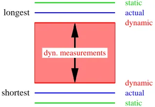
Figure 1.1 Static and dynamic analysis compared to actual execution time . . . 3
Figure 2.1 CheckerMode in Action . . . 14
Figure 2.2 CheckerMode Design . . . 15
Figure 2.3 Control Flow Graph of Toy Benchmark and Measured Cycles . . . 19
Figure 2.4 Measured Cycles (Aggregate Technique) for Synthetic Benchmark . . . 20
Figure 2.5 Timing Results for the ADPCM Benchmark . . . 21
Figure 2.6 Measured execution cycles for C-Lab Benchmarks . . . 22
Figure 3.1 Model used for description and capture of Snapshots . . . 27
Figure 3.2 Snapshot Captured using the DR Technique . . . 28
Figure 3.3 Definition of a Snapshot, based on the “Drain-Retire” mechanism . . . 29
Figure 3.4 Mechanism to Capture/Handle Structural Hazards . . . 30
Figure 3.5 Snapshot Merge Algorithm (DRM) . . . 34
Figure 3.6 Merging using the DRM Algorithm . . . 35
Figure 3.7 Incorrect Merge . . . 36
Figure 3.8 Merging Reservation Stations . . . 37
Figure 3.9 Merge for Multiple Snapshots . . . 37
Figure 3.10 Anomaly Effects on Merge . . . 38
Figure 3.11 Case 1 (a) (i)t′kis greater thantR{i}. . . 40
Figure 3.12 Case 1 (a) (ii)t′ kis less thantR{i}. . . 40
Figure 3.13 Case 2 (a) (i)t′kis less thantR {i}. . . 41
Figure 3.15 Case 3 (a) neithert′
knortR{i}change . . . 42
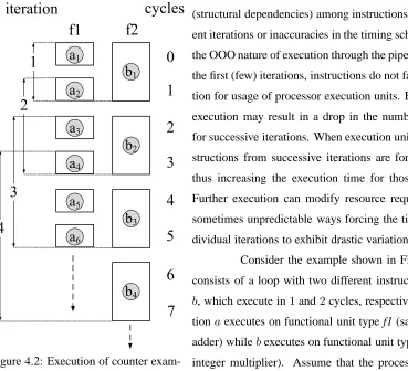
Figure 4.1 Counter example against use of only fixed point timing . . . 50
Figure 4.2 Execution of counter example through the pipeline . . . 50
Figure 4.3 A Second Fixed Point . . . 53
Figure 4.4 Alternative Execution Scenario for counter example . . . 54
Figure 4.5 Synthetic Benchmark for Analyzing Stable state of Reservation Stations . . . 55
Figure 4.6 CFG . . . 56
Figure 4.7 Measured execution cycles for loop path compositions (SRT bubblesort function) 57 Figure 4.8 Complete execution cycles for C-Lab Benchmarks – including loop WCECs . . . 61
Figure 4.9 δ’s for two and three level compositions for nine loops in ADPCM benchmark . . . 62
Figure 5.1 Static Timing Analysis Framework . . . 69
Figure 5.2 Numeric Loop Analysis Algorithm . . . 70
Figure 5.3 Use of Parametric Timing Analysis . . . 71
Figure 5.4 Parametric Loop Analysis Algorithm . . . 71
Figure 5.5 Syntactic and Semantic specifications for constraints on analyzable loops. . . 73
Figure 5.6 Example of an outer loop with multiple paths . . . 74
Figure 5.7 WCET Bounds as a Function of the Number of Iterations . . . 76
Figure 5.8 Flow of Parametric Timing Analysis . . . 77
Figure 5.9 Example of using Parametric Timing Predictions . . . 78
Figure 5.10 Experimental Framework . . . 81
Figure 5.11 Energy consumption for PCG Wattch Model – Dynamic Energy consumption . . . . 87
Figure 5.12 PCGL-W – Leakage Consumption from the Wattch Model . . . 88
Figure 5.13 PCGL – Leakage Consumption from the Wattch Model . . . 89
Figure 5.15 Comparison of Dynamic Energy Consumption for ParaScale-G and Lookahead . . 93
Figure 6.1 Edges and Nodes in the Timing graph . . . 104
Figure 6.2 Synchronization constructs . . . 105
Figure 6.3 Deadlocks in Timing Graphs . . . 105
Figure 6.4 Sample code to illustrate creation of the Timing Graph . . . 106
Figure 6.5 Timing graph created by application of various information gathering techniques . 108 Figure 6.6 Two Point-of-View Simplifications . . . 111
Figure 6.7 Remove direct red edges . . . 112
Figure 6.8 Move outgoing red edges to successor . . . 113
Figure 6.9 Move incoming red edges to predecessor . . . 114
Figure 6.10 Outcome of graph transformations . . . 115
Figure 6.11 Multiple producer-consumers . . . 115
Figure 6.12 Converting Blue edges to Red – creating futures . . . 116
Chapter 1
Introduction
Every year, billions of microprocessors are sold for use in embedded systems [120]. This is in sharp contrast to a few hundred million desktop processors that are sold in the same time-frame. From automobiles to medical equipment, thermostats to space shuttles, embedded systems are all around us. Moreover, the use of embedded systems is increasing, if anything, with the advent of “Cyber-Physical Systems” (CPS), which can be described as “integrations of computation with physical processes.” Hence, cyber-physical systems affect and are affected by the physical world and the environment that they operate in. The modern automobile and even smart homes fall into this category. They are typically comprised of networks and combinations of smaller embedded systems that perform specific tasks.
1.1
Real-Time Systems
The software and hardware used for embedded and cyber-physical systems, in general, must be validated, which traditionally amounts to checking the correctness of the input/output rela-tionship. Many such systems also impose timing constraints on the execution times of constituent tasks. Violations of these constraints (often referred to as “deadlines”) could lead to fallouts that are dangerous to users, the environment or both. Such systems are commonly referred to as “real-time systems”, and they impose temporal constraints on computational tasks to ensure that results are available on time. Often, approximate results supplied in time are preferred to more precise results that may become available late, i.e., after the passage of deadlines.
heavy braking. The driver is able to maintain control by the ABS as it allows the wheel to roll for-ward. In fact, recent versions not only perform the ABS functionality but also Electronic Brakeforce Distribution (EBD), Traction Control System (TCS), Electronic Stability Control (ESC), etc.. The ABS system is a classic example of a real-time, embedded system that we encounter in everyday life. If a driver must hit the brakes of a car in an emergency, then the ABS must kick in and function correctly in the milliseconds (perhaps even microseconds) time-frame. It is absolutely useless if it functions correctly, say ten seconds after the brakes have been pressed – in fact, a failure to operate in the short, required duration might result in a loss of human life and/or damage to property. Nu-clear reactor controls, electronic engines, modern avionics – all of these applications fall under the purview of real-time systems and have stringent design criteria. They require advance knowledge of the properties of and guarantees on the behavior of the system, the most critical of which is that no task in the system misses its deadline.
1.2
Worst-Case Execution Time (WCET)
Schedulability analysis [77] is used to guarantee that a given system of real-time tasks will be able to meet its deadlines on a particular hardware system. One critical piece of informa-tion required for such analysis is the “worst-case execuinforma-tion time” (WCET) of each task, which is defined as
“the guaranteed worst-case time taken by the task to execute on a specific hardware platform.”
The process of determining the WCET of a task is known as “timing analysis” and is often charac-terized as being either (a) static timing analysis or (b) dynamic timing analysis.
1.3
Timing Analysis
the analysis. Of course, even a tight bound has to be a safe bound in that it must not underestimate the true WCET; it may only match or exceed it.
Static timing analysis [14, 15, 26, 27, 34, 36, 49, 52, 53, 59, 73, 74, 82, 84, 89, 94, 97, 103, 119, 126, 133] techniques suffer from the drawback that they are either overly pessimistic or impose severe constraints on the types of code that may be analyzed (e.g., known upper bounds on loops, absence of function pointers and no heap allocation). If such an analysis is pessimistic, as shown in Figure 1.1, then system resources may be wasted. Bounds on execution times require constraints to be imposed on the tasks (timed code), the most striking of which is the requirement to statically bound the number of iterations of loops within the task. Complex architectural features, such as out-of-order (OOO) processing [96] and branch prediction [113], are often beyond the reach of static analyses, mainly due to the fact that they introduce non-determinism into the task code. These issues cannot be resolved at compile time, thus forcing real-time system designers to completely avoid the use of such processors.
Dynamic timing analysis methods [14, 15, 19, 119, 125, 127], on the other hand, are either trace-driven, experimental or stochastic in nature. They are unable to guarantee the safety of WCET values obtained [126]. Architectural complexities, difficulties in determining worst-case input sets and the exponential complexity of performing exhaustive testing over all possible inputs are also reasons why dynamic timing analysis methods are unsafe and, hence, infeasible in general. The threat of dynamic methods is that the execution time of tasks might actually be underestimated (as shown in Figure 1.1), which can result in serious errors during system operation, implying potentially dangerous fallouts.
actual
dynamic
static
static
dynamic
actual
longest
shortest
dyn. measurements
Figure 1.1: Static and dynamic analysis compared to actual execution time The objective of any timing analysis technique
is to approximate the worst-case actual execution time of a task, i.e., the longest possible execution time consid-ering all inputs and hardware complexities, deterministic or not. The more closely this value is approximated, the easier it is to design the system in an accurate, safe and efficient manner in terms of resource usage. Determina-tion of the WCET bounds of a task is a non-trivial process due to a variety of reasons, broadly classified into:
2. software complexities: non-determinism of inputs, complexity of task code, etc.
This work addresses these shortcomings on both fronts – hardware as well as software. Section 1.4 briefly discusses novel techniques to tackle hardware and architectural complexity while Section 1.5 introduces techniques to relax constraints imposed on task code. Section 1.6 introduces techniques aimed at analyzing complex embedded software – containing multiple threads that could potentially be distributed in nature. It also demonstrates applications where timing analysis tech-niques could be utilized to analyze complex systems. All of these techtech-niques utilize the interactions and passing of information between hardware and software to increase the accuracy of the analysis. The main idea is that a single source of information (such as only static or only dynamic analysis methods) is not sufficient for analyzing modern embedded systems that are inherently complex. Thus, novel methods that utilize information from multiple sources is required for a more complete analysis.
1.4
Tackling the Complexity of Contemporary Processors
A serious handicap in performing static timing analysis is the complexity of modern pro-cessors and their functional units. Various features that decrease average execution times for tasks are often detrimental for worst-case timing analysis. Out of order (OOO) processing [96] and branch prediction [113] are two important features in modern processors that introduce non-determinism to task execution, which cannot be resolved at compile time [12, 23, 35]. Other issues that increases the complexity of the analysis are the presence of statically indeterminate loops in task code and timing anomalies [13,79,81,109]. Hence, designers of real-time systems are often forced to use less complicated, older and inherently less powerful processors. While this guarantees determinism, it neglects performance. The following section (1.4.1) introduces the concept of “hybrid” timing anal-ysis that utilizes interactions between a software timing analyzer and run-time information from the actual microprocessor to obtain tight WCET estimates on contemporary processors.
1.4.1 CheckerMode
details as checkpoints of the processor state, also called “snapshots”. This information is then com-municated to a software module. The software module stores the various checkpoints (“snapshots”) and also drives the execution of the processors along statically determined paths to capture accurate timing information for each of them. The checkpoints are used to track back along the various exe-cution paths and to restart along a different path if necessary. The exeexe-cution times obtained for each of the paths is analyzed and combined by the software driver to calculate an accurate WCET for the entire module/program.
Decisions on where to obtain snapshots, the details required for a snapshot, etc. are made by the software driver. The timing results for each straight-line path are fed back to the software module. The software module, similar to a static (numeric) timing analyzer, then combines the timing results for individual paths to obtain a bound on WCET for the entire task. The cache states, the state of the branch predictor, the pipeline, etc., for each of the paths, are also considered while performing these calculations. To time an alternate path, the information from the previous checkpoint is then restored onto the processor function units to reflect the state of the system when the choice between the paths was made.
The ability to capture these snapshots is disabled during normal execution, so as to not interfere with regular program execution. The approach is evaluated by implementing additional micro-architectural functionality (the ability to capture snapshots, to restore a previous snapshot on to the processor function units and to obtain accurate timing results for parts of the program) on a customized SimpleScalar [22] framework that is configured in a manner similar to modern processor pipelines. Techniques to reduce the complexity of analysis for loops to ensure that the analysis overhead is independent of the number of loop iterations are also introduced. The ability of this analysis to correctly account for “timing anomalies” that could occur during out-of-order execution is also shown. To the best of my knowledge, this method of using a hardware/software co-design technique to obtain accurate WCETs for modern out-of-order processors is a first of its kind.
1.5
Relaxing Constraints on Embedded Software
that can be used in real-time systems. This type of timing analysis is referred to as numeric timing analysis [49, 52, 53, 94, 132, 133] since it results in a single numeric value for WCET given the upper bounds on loop iterations. The constraint on the known maximum number of loop iterations is removed by parametric timing analysis (PTA) [124], which is used in the ParaScale infrastructure, introduced in Section 1.5.1.
1.5.1 ParaScale
Parametric timing analysis permits variable-length loops. Loops may be bounded byn
iterations as long asnis known prior to loop entry during execution. Such a relaxation widens the scope of analyzable programs considerably and facilitates code reuse for embedded/real-time ap-plications. This work describes (a) the application of static timing analysis techniques to dynamic scheduling problems and (b) assesses the benefits of PTA for dynamic voltage scaling (DVS). This work contributes a novel technique that allows PTA to interact with a dynamic scheduler while dis-covering actual loop bounds during execution prior to loop entry. At loop entry, a tighter bound on the WCET can be calculated on-the-fly, which may then trigger scheduling decisions synchronous with the execution of the task.
The benefits of using PTA to analyze code sections is evaluated by measuring power savings in the system. Power savings are typically achieved by means of dynamic voltage scaling (DVS) or dynamic frequency scaling (DFS) techniques. The ParaScale infrastructure utilizes a combination of inter, and intra-task DVS techniques to achieve power savings. ParaScale uses the results of PTA by using parametric formulae, evaluated at run-time, to make dynamic decisions on the amount of execution completed, amount of slack left, and frequency/voltage scaling to reduce power consumption. An intra-task scheduler is used for this purpose. Hence, ParaScale provides the ability to evaluate the benefits of PTA on a system.
1.6
Analysis of Distributed Embedded Systems
Cyber-physical systems operate on a variety of embedded hardware ranging from 8-bit microcontrollers to sophisticated multicores. Knowledge of the temporal behavior of an application is hidden inside the application logic, where it is extremely difficult to extract, analyze and model for any given hardware. While static and dynamic timing analyses are used to obtain the worst-case execution times (WCETs) for real-time applications, they may not be able to provide a complete pic-ture of a program. This is particularly true in the case of larger, more complex programs. Programs that contain function pointers are typically out of reach of static analyzers. Dynamic analyzers are unable to gauge the true nature of the program and have shown to be unsafe – i.e., they may under-estimate the WCET of the program, which could lead to dangerous effects. If the application uses concurrency constructs, such as signals, locks or mutexes, then neither of these techniques can fully analyze the application.
The work presented here studies the use of combinations of a variety of techniques to form the complete picture of the structure and execution characteristics of a distributed embedded application. The results obtained are collected to create timing graphs, the topology of which can be studied to extract meaning about the application. This information can then be used to
• provide information to the designers of the system to be used to identify problematic areas in the application and to
• tailor the amount of parallelism in the system so that the same application can execute on small embedded microcontrollers as well as large, modern multicore processors.
1.7
Organization
The remainder of this dissertation is loosely split into three parts:
2. ParaScale: Chapter 5 describes the ParaScale infrastructure used to relax constraints on em-bedded software, the results from which are used to attain power savings (published in RTSS 2005 [89] and the TECS journal [88]).
3. Distributed Embedded Systems: Chapter 6 discusses techniques used to analyze distributed embedded systems (published in ECRTS 2008 [85]).
Chapter 7 presents the related work. Chapter 8 presents ideas for future work while Chap-ter 9 presents the conclusion.
1.8
Hypothesis
Modern embedded systems with timing constraints are too complex to be analyzed by any single technique alone due to the non-determinism introduced by hardware features as well as complexities in software. Hence, the hypothesis of this dissertation is that
by employing a combination of multiple analysis techniques, multiple sources of infor-mation and constant interactions between hardware and software it becomes feasible to gauge the worst-case behavior of modern embedded systems that utilize contemporary processors and complex software constructs.
The analysis presented is constrained to
1. analyzing out-of-order processor pipelines, correct handling of timing anomalies and loops around them; to
2. providing power savings by removing constraints that enforce statically determinate loop bounds; and to
Chapter 2
CheckerMode – Tackling the Complexity
of Modern Processors
2.1
Summary
A limiting factor for designing real-time systems is the class of processors that can be used. Typically, modern, complex processor pipelines cannot be used in real-time systems design. Contemporary processors with their advanced architectural features, such as out-of-order execu-tion, branch predicexecu-tion, speculaexecu-tion, prefetching, etc., cannot be statically analyzed to obtain tight WCET bounds for tasks. This is caused by the non-determinism of these features, which surfaces in full only at runtime. This chapter introduces a new paradigm to perform timing analysis of tasks for real-time systems running on modern processor architectures. Minor enhancements to the pro-cessor architecture are proposed to enable this process. These features, on interaction with software modules, are able to obtain tight, accurate timing analysis results for modern processors.
2.2
Introduction
are often detrimental for worst-case timing analysis. Out of order (OOO) processing [96] and branch prediction [113] are two important features in modern processors that introduce non-determinism to task execution, which cannot be resolved at compile time [12, 23, 35]. Hence, designers of real-time systems are often forced to use less complicated, older and inherently less powerful processors. In this chapter, techniques to bridge this gap by means of the CheckerMode infrastructure are pre-sented. CheckerMode combines the best features of both, static and dynamic analysis, to create a novel hybrid mechanism for WCET analysis.
Minor enhancements to the micro-architecture of future processors are presented that will aid in the process of obtaining accurate WCET bounds. A “checker mode” is added to processors that will, on demand, capture varying levels of information as “snapshots” of the processor state. This information is communicated to a software module that stores the various snapshots and also drives the execution of instructions in the processor along statically determined paths. Accurate timing information for each path is then captured. These snapshots are also used to backtrack to an earlier state and then restart along a different path. Execution times obtained for each path are analyzed and then combined by the software driver to calculate an accurate WCET for the entire program/function.
Decisions on where to obtain snapshots, the level of detail required for each snapshot, etc. are made by the software controller (“driver”). Timing results for each straight-line path are then fed back to the software module. The software module (similar to a static/numeric timing analyzer), then combines the timing results for individual paths to obtain a bound on WCET for the entire task. The cache states, the state of the branch predictor, the pipeline, etc., for each of the paths, are also considered while performing these calculations. To time an alternate path, the information from the previous snapshot is restored onto the processor function units to reflect the state of the system when the choice between the paths was made.
The ability to capture these snapshots is disabled during normal execution, so as to not interfere with regular program execution. The approach is evaluated by implementing additional micro-architectural functionality (the ability to capture snapshots, to restore a previous snapshot on to the processor function units and the ability to obtain accurate timing results for parts of the program) on a customized SimpleScalar [22] framework that is configured in a manner similar to modern processor pipelines.
2.2.1 Plausibility of the approach
The proposed hardware enhancements are realistic. The support for speculative execution due to dynamic branch prediction, precise exception handling and precise hardware monitoring, and even most of the internal buffers required by the CheckerMode design already exist in modern high-end embedded processors. For example, the ARM-11 features out-of-order execution, dy-namic branch prediction, and precise traps, which requires shadow buffers (for registers, branch history tables etc.) [28] in order to recover to a prior execution state. In addition to these fea-tures, the Intel x86 architecture supports Precise Event Based Sampling (PEBS) with user access to selected shadow buffers [114]. Future processor extensions also make heavy use of checkpoint buffers [29, 30, 66]. CheckerMode’s design will make such buffers uniformly available to the user. Enhancements to the ALU and branch logic to handle the new semantics for NaN (Not-A-Number) operands are required by CheckerMode (see Section 2.3), which are minor modifications compared to the space and complexity of the already existing shadow buffers. In fact, most processors already implement a NaN representation for floating point values (and an equivalent bottom value for inte-gers), which is generated when undefined arithmetic (e.g., divide-by-zero) is performed and results in an exception (trap). The sole modification suggested would be to gate the exception, i.e., suppress it in CheckerMode, and proceed with arithmetic operations in the presence of NaN values.
2.2.2 Processor Vendor Limitations
One other shortcoming of static timing analysis approaches developed so far is given by their targeting of a generic processor type based on vendor-supplied design details. In such an approach, each new processor design requires that the timing model be manually adapted while the CheckerMode technique automatically adapts with changing processor details. Furthermore, such timing models are only as good as the information provided by the vendor, which may not reveal all details of the design. For example, Intel’s CPU stepping index indicates subtle processor modifications within the same CPU family but does not reveal all details.
protect their IP while providing a method to obtain highly accurate timing. Since CheckerMode observes the execution time on an actual processor, such variability is captured.
CheckerMode widens the scope of processors that may be used in a real-time system. Contemporary processors with state-of-the-art functionality and performance may subsequently be used in real-time systems. This also changes the landscape for timing analysis in that more accurate results can be obtained on modern pipelines without risk of losing functionality. In a world of increasingly specialized components, the idea that some processors could be designed specifically for use in real-time and embedded systems has already caught on, e.g., with designs that customize generic core, such as the ARM-7/9/11 licensed by Qualcomm and many others. This is especially true in the design and testing phases for the real-time systems being created. These processors would not behave any differently during normal execution but would only have the additional characteristic that more information can be gathered from them during the analysis phase. Hence, there is an assurance that the additional features will not further complicate the analysis.
2.2.3 Assumptions
CheckerMode, in its current state only addresses the unpredictable nature of out-of-order instruction execution in contemporary high-end embedded processor pipelines. Other complexities, such as memory hierarchies, including caches, and dynamic branch prediction are beyond the scope of this initial work and will be addressed in the future. Tasks are analyzed in isolation. Preemptions and cache-related preemption delays, handled by orthogonal work [105], could be incorporated in the future and should not require any changes to the CheckerMode approach since their analysis occurs at a higher level.
2.2.4 Organization
This chapter is organized as follows. Section 2.3 introduces the CheckerMode infras-tructure. Section 2.4 explains the experimental setup. Section 2.5 enumerates the results from the experiments while Section 2.6 summarizes the high-level contributions.
2.3
CheckerMode
the microarchitecture while closely interacting with software to obtain WCET bounds. The idea is to design embedded processors, that in addition to executing software normally (in a so-called deployment mode), are capable of executing in a novel CheckerMode that supports timing analysis. CheckerMode provides cycle-accurate bounds on the WCET by assessing alternate exe-cution paths in a program. In deployment mode, a processor executes along just one path following a conditional branch; which path is executed may depend on the input data. In CheckerMode, a processor no longer proceeds with conventional data-driven execution. Instead, it executes all alter-nate paths, one at a time, following each conditional branch in order to find the path with the largest execution time. Before the execution of each alternate path, the original execution context (includ-ing caches, branch history tables etc.) is restored to correctly simulate the effect of alternations in isolation from one another. These low-level WCET results are propagated inter-procedurally in a bottom-up fashion (over the combined control-flow and call graphs) until the WCET for an entire task has been computed.
Consider a task that consists of a number of feasible execution paths. The execution times for these paths are obtained by actual execution in CheckerMode through the processor pipeline. The execution time for each path is then captured and stored. When conditional execution arises, all alternate paths are timed separately on the pipeline. The timing information as well as the “state” of the processor (determined by the cache state, branch predictor state, register state, etc.) are combined when alternate paths join. The combination is performed such that the state that results from the combination must not underestimate the execution time of the alternate paths or even the future execution of the task. A set of timing schemes for individual paths as well as combinations of paths, derived from this methodology, is discussed in the results section.
Prior to the execution of alternate paths, a “snapshot” of the processor state is obtained and stored. After the execution of one of the alternate paths, its state is recorded for later combination with other paths. Then, the state of the processor is restored to the one that existed before the path started executing. This is achieved by restoring the state (e.g., of each of the parts of the pipeline) from the previously captured snapshot.
block 4, another snapshot (snapshot 1) of the processor state is captured and stored. The time taken to execute this path is also measured and sent to the timing analyzer. The program counter is then reset to basic block 1 (the branch condition) to trace execution down the other side (not-taken) and to subsequently capture the execution time for that path. Before execution proceeds along the not-taken path, the state of the processor is restored to the previously saved snapshot (snapshot 0). This isolates the effects of execution of one path from that of another. Once the processor state from snapshot 0 is written back, execution from basic block 1 proceeds down the not-taken path (1 →
3→ 4) before the processor state (snapshot 2) and execution time are captured once again. Only then can the CheckerMode unit shift its focus to the code that follows basic block 4. For execution to proceed from basic block 4, the processor must be set to a consistent state. At this point, it is necessary to perform a merge of the snapshots from the two paths. The merge must be performed such that the worst-case behavior of the subsequent code is preserved. Hence, we must merge the state of all processor units captured in preceding snapshots. Once a merge has been performed, the new state must be written back to the processor and execution continues from that point on.
Figure 2.1: CheckerMode in Action
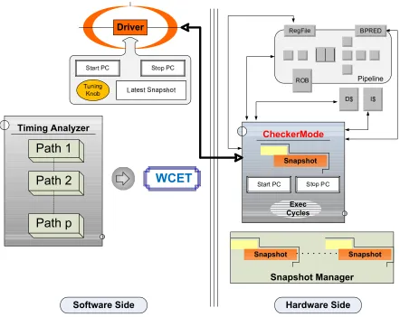
The hardware-supported Checker-Mode is complemented by software analysis to govern checker execution (see Figure 2.2). The analysis controller (or driver) steers checker execution along distinct execution paths, i.e., it indicates which direction a branch along the path should take till all paths have been tra-versed. The timing information and the states of the processor obtained for each possible path are then used by a “timing analyzer” to obtain the WCET for the entire task (or even certain code sections). Each of these is explained in the following sections.
2.3.1 Processor Enhancements
Figure 2.2: CheckerMode Design
together with the timing for the path.
Hence, the novel CheckerMode unit of the processor supports the following functions: (a) Capture snapshots of the processor state and communicate them to the software controller. A snapshot captures the current state of the processor pipeline, associated functional units and caches, ROB, etc.
(b) Reset the processor to a previously saved state. Given an earlier snapshot, the state of the processor pipeline, caches, functional units, etc., is overwritten with information from the stored snapshot.
(c) Start and stop execution between any two program counter (PC) values. This includes support to calculate the number of cycles elapsed between the execution of the given start and stop PCs.
CheckerMode unit must be able to read and write to the various functional units of the processor. The CheckerMode unit is controlled by the driver (or controller) on the software side.
2.3.2 Software Overview
The left-hand side of Figure 2.2 illustrates the various components that make up the soft-ware side of the design. It consists of the following components:
Timing Analyzer (TA): The TA breaks down the task code into a control-flow graph (CFG) and then extracts path information from it. Using this information, the TA is able to determine the start of alternate execution flows – points where snapshots must be obtained. It also provides the start and stop PCs to the driver and obtains the WCET and processor state for that particular path from the driver.
Snapshot Manager (SM): The SM maintains various snapshots that have been captured as well as the PCs at which they were obtained. SM abstractions can be integrated into the processor as depicted in Fig. 2.2, or, alternately, into the driver within the software controller.
Driver: The driver controls the hardware side of the system. It instructs the hardware on when to start and stop execution, when snapshots must be captured, and when the state of the processor must be reset to a previous snapshot, as detailed below.
The input to the TA is the executable of a task. Assembly information is extracted (with PCs) from an executable and then converted to internal representations as combined control-flow and call graphs. The start and stop PCs provided by the TA encapsulate a single path. The TA, the driver, and the SM interact to decide which snapshot corresponds to which path, which PC, etc., and thereby control program execution.
The TA is responsible for obtaining the final WCET for the entire program as well as various program segments (functions/scopes). It “combines” the information from various paths (execution time, pipeline state, etc.) for this purpose. The driver, also part of the software system, is described in more detail below.
2.3.3 Driver/Analysis Controller and Tuning
the start/end points of the path to be timed. It also stores the latest captured snapshot. The driver maintains information about which instruction is a branch and where snapshots need to be captured. It also relays information in the other direction – from the hardware to the timing analyzer – e.g., the path execution time.
2.3.4 False Path Identification and Handling
A principal component of the analysis controller is a queue of saved processor contexts guiding path exploration. In some cases, not all paths need to be considered, as implied by these contexts. For example, a path can be dropped if static analysis concludes that this execution path cannot be executed (i.e., it is a “false path”). Similarly, if a path can be shown to be shorter than some other paths that have already been explored, then again this path can be dropped from the queue.
2.3.5 Loop Analysis Overhead
We can reduce the complexity of determining the WCET by partial execution of loops such that the analysis overhead is independent of the number of loop iterations. The approach of a fix-point algorithm from prior work [10] is used to determine a stable execution time for the loop body. Now loop executions can be steered such that paths of a loop body are repeatedly executed till a stable value is reached. This technique is explained in detail in Chapter 4.
2.3.6 Input Dependencies
In CheckerMode, input-dependent register values are deemed unknown, which is inter-nally represented in a manner similar to NaN (not-a-number) values already existing in floating point units (and similarly for integer ALUs). Operations on unknown values are straightforward: if any input is unknown then the output is also unknown. It is necessary to represent the known/unknown status of condition codes at the bit level. A branch condition based on an unknown value then in-dicates a need to consider alternate paths. Conversely, concrete (known) values are evaluated as always and input-invariant branches will result in timing of only the taken execution path.
rresult=
NaN if ra=NaN W rb=NaN
ra+rb otherwise
Hence, any operation with NaN as one of the operands will result in NaN (unless the result is independent of that particular operand, e.g., multiplication with 0 will always result in 0). Similar enhancements are developed for other instructions that depend on input-dependent or
memory-loaded operands.
2.3.7 Analysis Overhead
The process of timing analysis now amounts to timing sequences of paths by saving and restoring snapshots of processor state in a coordinated fashion. While this process can be lengthy, it still remains independent of the input to the program, and in the worst-case, can be run overnight. Since this is an offline task to be performed during system design and validation, the cost is sec-ondary and does not affect the dynamic, run-time behavior of the system. Sometimes such a full verification of WCET bounds is generally only warranted after extensive code changes during de-velopment and for each software deployment, including system upgrades. In practice though, safety requirements of hard real-time systems demand that this level of verification be carried out for even the smallest changes. During system development, it could be performed after larger changes from time to time but must finally be performed fully at least once before the final deployment.
2.4
Experimental Framework
The key components of the CheckerMode design were implemented in the SimpleScalar processor simulator [22]. This cycle-accurate simulator can be configured for the various processor and branch prediction schemes. SimpleScalar was used in three configurations:
1. Simple-IO (SimIO) simulates a simple, in-order (IO) processor pipeline (pipeline width 1, instruction issue in program order)
2. Superscalar-IO(SupIO) with a pipeline width (from fetch to retire) of 16 and in-order instruc-tion execuinstruc-tion
Table 2.1: C-Lab Benchmarks
Benchmark Function
ADPCM adaptive pulse code modulation CNT Sum and count of positive and
nega-tive numbers in an array. FFT Finite Fourier Transform LMS Least Mean Square Filter
MM Matrix Multiplication
SRT Implementation of Bubble Sort.
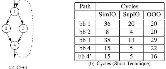
The C-Lab benchmarks [25] (enumerated in Table 2.1) were used for the experiments. Experiments were also conducted on a synthetic benchmark whose control-flow structure is depicted in Figure 2.3(a). Execution time for paths is measured using four different techniques, extending from the use of basic blocks (BB) [5] to paths (sequences of consecutive BBs):
1. Short measures the execution time of a single BB, starting from the time that any instruction in the BB/path moves into the execute stage of the pipeline and finishing when the last instruction of the BB/path exits from the retire stage.
2. Path-Short captures the execution time for paths (concatenated BBs) using the “short” tech-nique so that timing starts at the first BB and ends with the last BB in the path.
3. Path-Aggregate captures the time for concatenated paths so that timing starts at the first BB of the first path and ends with the last BB of the last path.
4. Program-Aggregate includes the time from the start of the execution (main function) to the end of a BB in the path being timed, starting when the first instruction in the main function is fetched and finishing when the last of the path exits from the retire stage.
1
2 3
4
(a) CFG
Path Cycles
SimIO SupIO OOO
bb 1 36 20 20
bb 2 8 4 20
bb 3 38 13 29
bb 4 15 5 22
bb 4’ 15 5 16
(b) Cycles (Short Technique)
2.5
Results
The results obtained for the “short” technique (Figure 2.3(b)) show that timings for the processor modes SimIO and SupIO accurately reflect the actual WCET bounds, both for single BBs and paths. However, the OOO results exceed those of SupIO, due to early out-of-order execution of some instructions in parallel with other instructions from prior BBs in the path. Timing is started when any instruction in the relevant path comes into the execute stage of the pipeline, which could very well happen even when the previous path is not complete due to the inherent nature of out-of-order execution. Since timing only stops when the last instruction in the current path retires, the total execution time includes some time from execution of instruction in the previous path. Hence, the observed execution time includes cycles for instructions from earlier paths, which were not supposed to be timed. Even timing multiple BBs of a path in sequence (“path-short” technique) does not alleviate this problem. bb4 and bb4’ represent the same code – the difference is the path taken to get to basic block 4. In the first case, the “then” case of the branch was selected and in the second case, then “else” case was followed.
In contrast, the “aggregate” technique (Figure 2.4) reflects the time from instruction fetch (instead of execute) and also times longer paths. This addresses the above problem of early execu-tion by some instrucexecu-tions because in the long run, timing longer paths reduces the inaccuracies from interactions between individual instructions . Results show a strict ordering of execution cycles for
SimIO ≥ SupIO ≥ OOO, as expected by the amount of instruction parallelism, since time is measured from the first fetch of an instruction. The differences between paths (“delta”) provide a bound on the number of cycles for the tail BB in the path, thus excluding any pipeline overlap with prior BBs. Hence, these delta values can be used to assess the amount of cycles attributed to specific BBs alone. They also adhere to the same strict ordering. In general, such timing results are only valid in the same execution context/path, i.e., different BB sequences of one path may influence subsequent BBs in the control flow.
Path SimIO delta SupIO delta OOO delta
BB1 82 BB1-BB0=56 66 BB1-BB 0=4 47 BB1-BB0=1
BB1,2 114 BB1,2-BB1=32 94 BB1,2-BB1=28 59 BB1,2-BB1=12
BB1,3 241 BB1,3-BB1=159 131 BB1,3-BB1=65 92 BB1,3-BB1=45
BB1,2,4 151 BB1,2,4-BB1,2=37 97 BB1,2,4-BB1,2=3 61 BB1,2,4-BB2=2 BB1,3,4 278 BB1,3,4-BB1,3=37 134 BB1,3,4-BB1,3=3 94 BB1,3,4-BB1,3=2
0 500 1000 1500 2000 2500 3000 3500 4000
1 4 7 10 13 16 19 22 25 28 31 34 37 40 43 46 49 52 55 58
Path Id
C
yc
le
s
SimIO SupIO OOO
(a) Execution cycles for each Path
Function Num. Instructions Num. Paths
abs 18 2
filtep 35 1
logsch 36 2
logscl 37 2
filtez 48 2
uppol1 49 8
uppol2 58 8
quantl 65 6
main 88 4
upzero 122 5
decode 317 4
encode 330 16
(b) Num. of Instructions & Paths for ADPCM functions
Figure 2.5: Timing Results for the ADPCM Benchmark 2.5.1 C-Lab Benchmark Results
All paths from each of the C-lab benchmarks were extracted and then timed independently using the CheckerMode framework in each of the three configurations (SimIO, SupIO and OOO). Figures 2.5 and 2.6 summarize the results for the ADPCM, LMS and SRT benchmarks, respectively. ADPCM is the largest benchmark in the C-lab suite, with14functions and60paths, while LMS and SRT are smaller benchmarks with10paths each. Results are sorted in ascending order based on the timing results for the SimIO configuration. All three graphs show theSimIO≥SupIO≥OOO
ordering except for one path in the SRT benchmark, the reason for which is explained later. Table 2.2: Averaged WCECs for C-Lab Benchmarks
Benchmark SimIO SupIO % Savings OOO % Savings
ADPCM 1340 486 63.7 367 72.6
CNT 356 197 44.6 76 78.7
FFT 1047 439 58.1 288 72.5
LMS 839 457 45.6 236 71.9
MM 161 144 10.6 58 64.0
SRT 330.2 198 40.1 93 71.8
0 200 400 600 800 1000 1200 1400
1 2 3 4 5 6 7 8 9 10
Path Id C yc le s SimIO SupIO OOO
(a) LMS benchmark
0 100 200 300 400 500 600 700 800
1 2 3 4 5 6 7 8 9 10
Path Id C yc le s SimIO SupIO OOO
(b) SRT benchmark
Figure 2.6: Measured execution cycles for C-Lab Benchmarks
in the case of encode, a large number of paths as well. While there is enough parallelism in the code for SupIO and OOO to exploit, the SimIO configuration, with its in-order behavior and single width pipeline, is unable to scale as well as the other two configurations. This also shows that the number of dependencies between instructions in the two functions is not very high, as OOO is able to scale well to handle the larger instruction load.
The graph for LMS (Figure 2.6(a)) shows that all three configurations scale in a similar fashion for larger paths. It is interesting to note that the timing results for SupIO are approximately half of that for SimIO. Similarly, the timing results for OOO are approximately half that of SupIO. Similar results are seen for the SRT benchmark as well (Figure 2.6(b)), except for the shortest path (path 1). This path is so short that the effects described at the beginning of Section 2.5 become apparent – i.e., timing is started when the first instruction of the program is fetched and stopped when the final instruction is retired. Hence, the first instruction has to wait for a while before it is dispatched. When the paths are very short, the pipeline contains a large number of instructions that do not belong to the particular path being timed, hence bloating the results for pipelines with larger width. The single width SimIO configuration does not suffer from this problem as the instruction is
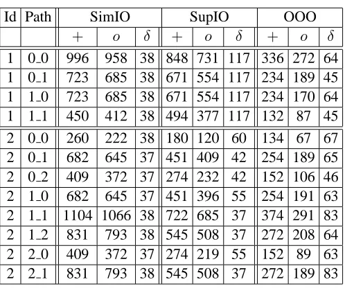
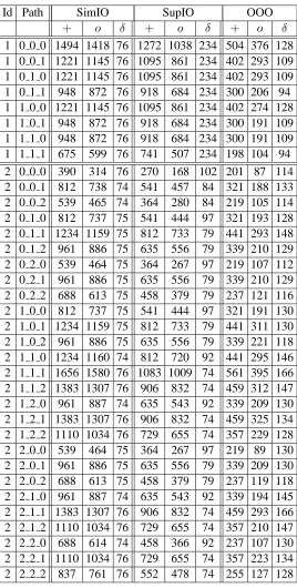
Table 2.3: Path-Aggregate Cycles (3 Iterations) for the Synthetic Benchmark
Path SimIO SupIO OOO
+ o δ + o δ + o δ
dispatched immediately after being fetched.
The FFT and MM benchmarks also show similar results. The results of all six benchmarks are summarized in Table 2.2. The second, third and fifth columns are the worst-case number of cycles for each benchmark averaged across all paths. The fourth and the sixth columns show the average savings for each benchmark for the preceding configuration (preceding row in the table) as compared to SimIO (column2). Specifically, the fourth column shows the average savings for SupIO over SimIO, and the sixth column shows the average savings for OOO over SimIO. These savings are based on the averages across all paths.
2.6
Conclusion
Chapter 3
Merging State and Preserving Timing
Anomalies in Pipelines of High-End
Processors
3.1
Summary
This chapter provides further insights into the CheckerMode idea presented in Chapter 2 by introducing novel pipeline analysis techniques for accurately capturing the worst-case behavior of real-time tasks, i.e., methods to capture (“snapshot”) pipeline state and to subsequently perform a “merge” of previously captured snapshots. This chapter also includes proofs that the pipeline analy-sis correctly preserves worst-case timing behavior on OOO processor pipelines. It also specifically shows that anomalous pipeline effects, effectively dilating timing, are preserved by these methods.
3.2
Introduction
Chapter 2 introduced the notion of “hybrid” timing analysis [86] called the CheckerMode infrastructure which combines the best features of both static and dynamic analysis to obtain accu-rate WCET estimates for real-time tasks running on modern microprocessors. This chapter,
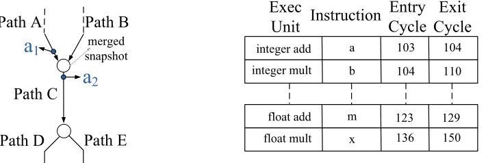
3. illustrates how two or more snapshots are “merged”, which occurs when multiple control paths “join” together;
4. prove that the mechanisms for capturing and merging snapshots are correct in that they retain all worst-case pipeline effects;
5. explains how the mechanisms to capture and merge snapshots are able to correctly handle “timing anomalies” [13, 79, 81, 109].
The remainder of this chapter is organized as follows: Section Section 3.3 introduces the notion of snapshots while Section 3.4 explains the models used for the analysis in this Chapter. Section 3.6 explains the techniques to capture the behavior of instructions in the pipeline. This is mainly aimed at capturing structural and data dependencies in an accurate manner. Section 3.5 details how a snapshot is captured while Section 3.7 provides the context on how these snapshots can used. Section 3.8 discusses how two or more snapshots are merged (before a join point in the control flow) so that the processor are reset to a consistent state for the following instructions. Section 3.9 proves that pipeline effects that modify timing will be retained post-merge. Section 3.10 develops a simple mechanism to merge register files. Section 3.11 discusses the details of the implementation. Finally, the conclusions are presented in Section 3.12.
3.3
Snapshots
Snapshots describe the state of the processor captured while performing timing analysis using the “hybrid” CheckerMode technique [86] to obtain the worst-case execution time for modern processor architectures. It typically consists of the state of each functional unit of the processor at a given point in time (t). This state includes, but is not limited to:
I pipeline state: in a generic sense, the state of instructions in the pipeline. Ideally, this state includes a description of which instructions are at what stage in the pipeline at timet. It also includes the contents of the register file.
III branch predictor state: similar to the cache state above: (a) complete branch history register and branch table contents; (b) delta from previous snapshot; or (c) a combination of the two. IV your favorite processor unit: state from any additional/future processor units that needs to be
captured to accurately characterize the worst-case behavior of the processor.
This chapter focuses on capturing the pipeline information of the processor for snapshots and not on caches, branch predictors, etc. Analysis of instruction caches is a solved problem, and any such analysis can be plugged into the CheckerMode framework to obtain better worst-case results. Analysis of data caches is a hard problem but some analysis does exist [93, 104, 123, 131], results from which can also be inserted into the CheckerMode framework to tighten the WCET results. Branch Predictor analysis is left for future work.
While capturing fine-grained details of instruction flow through the pipeline (defined above as “pipeline state”) would be ideal, practical difficulties prevent the process. Many changes to the design and implementation of the processor will have to be carried out to attain the ability to observe every single stage of the pipeline, instructions in flight, data forwarding, etc. Hence this chapter presents a novel technique devised to capture pipeline information, which, in essence, achieves the effect of characterizing the state of the pipeline at the given instant. This technique is named, the “drain-retire” (DR) technique. The DR technique is based on the idea that the only point of predictability in an out-of-order pipeline is at the retire stage. Since retire happens in-order, one can be sure that the retire order of instructions is deterministic. The DR technique is discussed in more detail in Sections 3.5 and 3.7.
3.4
Analysis Model
Figure 3.1(a) shows a section of the instruction stream that is executing through the pipeline. Let Sn be the last snapshot that was captured. Let “max” be the maximum number of instructions that can fit into the pipeline assuming that there are no dependencies between any of them. This is the theoretical upper bound for the pipeline capacity and is typically never achieved in practice – due to the existence of dependencies between instructions, which introduce bubbles in the pipeline.