Development of a Quantitative Decision Metric for Selecting the Most Suitable Discretization Method for SN Transport Problems.

(1)

ABSTRACT

SCHUNERT, SEBASTIAN. Development of a Quantitative Decision Metric for Selecting the Most Suitable Discretization Method for SN Transport Problems. (Under the direction of Yousry Y. Azmy.)

In this work we develop a quantitative decision metric for spatial discretization methods

of the SN equations. The quantitative decision metric utilizes performance data from selected test problems for computing a fitness score that is used for the selection of the most suitable discretization method for a particularSN transport application. The fitness score is aggregated as a weighted geometric mean of single performance indicators representing various performance

aspects relevant to the user. Thus, the fitness function can be adjusted to the particular needs of the code practitioner by adding/removing single performance indicators or changing their

importance via the supplied weights.

Within this work a special, broad class of methods is considered, referred to as nodal methods. This class is naturally comprised of the DGFEM methods of all function space

families. Within this work it is also shown that the Higher Order Diamond Difference (HODD)

method is a nodal method. Building on earlier findings that the Arbitrarily High Order Method of the Nodal type (AHOTN) is also a nodal method, a generalized finite-element framework

is created to yield as special cases various methods that were developed independently using

profoundly different formalisms.

A selection of test problems related to a certain performance aspect are considered: an

Method of Manufactured Solutions (MMS) test suite for assessing accuracy and execution time, Lathrop’s test problem for assessing resilience against occurrence of negative fluxes, and a

simple, homogeneous cube test problem to verify if a method possesses the thick diffusive limit.

The contending methods are implemented as efficiently as possible under a common SN transport code framework to level the playing field for a fair comparison of their computational

load. Numerical results are presented for all three test problems and a qualitative rating of

each method’s performance is provided for each aspect: accuracy/efficiency, resilience against negative fluxes, and possession of the thick diffusion limit, separately. The choice of the most

efficient method depends on the utilized error norm: in Lp error norms higher order methods

such as the AHOTN method of order three perform best, while for computing integral quantities the linear nodal (LN) method is most efficient. The most resilient method against occurrence

of negative fluxes is the simple corner balance (SCB) method.

A validation of the quantitative decision metric is performed based on the NEA box-in-box suite of test problems. The validation exercise comprises two stages: first prediction of

(2)

scores based on data obtained from the NEA benchmark problem. The comparison of predicted

and actual scores via a penalty function (ratio of predicted best performer’s score to actual best score) completes the validation exercise. It is found that the decision metric is capable of very

accurate predictions (penalty < 10%) in more than 83% of the considered cases and features penalties up to 20% for the remaining cases. An exception to this rule is the third test case NEA-III intentionally set up to incorporate a poor match of the benchmark with the “data”

problems. However, even under these worst case conditions the decision metric’s suggestions are

never detrimental. Suggestions for improving the decision metric’s accuracy are to increase the pool of employed data, to refine the mapping of a given configuration to a case in the database,

(3)

Development of a Quantitative Decision Metric for Selecting the Most Suitable Discretization Method forSN Transport Problems

by

Sebastian Schunert

A dissertation submitted to the Graduate Faculty of North Carolina State University

in partial fulfillment of the requirements for the Degree of

Doctor of Philosophy

Nuclear Engineering

Raleigh, North Carolina

2013

APPROVED BY:

Ilse Ipsen Dmitriy Anistratov

John Mattingly Rachel N. Slaybaugh

Co-chair of Advisory Committee

Yousry Y. Azmy

(4)

DEDICATION

(5)

BIOGRAPHY

Sebastian Schunert was born in Banteln, Germany on February 23, 1983. He attended the

Gym-nasium Alfeld (High School), graduating 2002. He started studying Mechanical Engineering in Braunschweig, Germany in Fall 2003 receiving his Vordiplom (B.S.) in 2005 and his Diplom

(M.S. equivalent) in 2008. From August 2007 until July 2008 he worked with Dr. Yousry Azmy

at The Pennsylvania State University. In January 2009 he started his Ph.D. under the super-vision of Dr. Yousry Azmy at North Carolina State University. His research interests include

(6)

ACKNOWLEDGEMENTS

First and foremost, I would like to thank my academic advisors, Dr. Yousry Azmy and Dr.

Rachel Slaybaugh, for their guidance during my time as an exchange student at The Pennsyl-vania State University, and later as a Ph.D student at North Carolina State University.

I want to express gratitude towards my current and former office-mates: Jose Duo, Max

Rosa, Kursat Bekar, Mike Ferrer, Andrew Bielen, Dan Gill, Josh Hykes, Sean O’Brien, Sameer Vhora, Brian Powell and Noel Nelson. Typically forgotten in other’s acknowledgement lists but

kindly remembered in this one: Joe Zerr. Without you I might have finished a lot quicker, but

it would not have been half as much fun.

To my parents - you instilled in me all the attributes I needed to succeed. I would like to

thank you for your support and faith in me during the time I spent at NC State.

(7)

TABLE OF CONTENTS

LIST OF TABLES . . . .viii

LIST OF FIGURES . . . ix

Chapter 1 Introduction . . . 1

1.1 The Transport Equation . . . 5

1.2 Solution of the One-GroupSN Equations . . . 8

1.2.1 Space-Angle Mesh Sweep . . . 8

1.2.2 Source Iterations . . . 9

1.2.3 GMRES Solution ofSN equations . . . 10

1.3 Thesis Outline . . . 10

Chapter 2 Review of Spatial Discretization Methods . . . 12

2.1 General Classification of Spatial Discretization Methods . . . 12

2.2 Discontinuous Finite Element Framework . . . 16

2.2.1 The Weak and Strong Form of theSN Transport Equation . . . 18

2.3 Review of Spatial Discretization Methods for theSN Equations . . . 20

2.3.1 Diamond Difference Type Methods . . . 20

2.3.2 The Discontinuous Galerkin Finite Element Method (DGFEM) . . . 25

2.3.3 Simple Corner Balance Method . . . 30

2.3.4 Transverse Moment Type Methods . . . 33

2.4 Nodal Finite Element Framework . . . 40

2.4.1 HODD as Petrov-Galerkin FEM . . . 41

2.4.2 AHOTN as DPGFEM Method . . . 44

2.5 Summary of Spatial Discretization Schemes . . . 45

Chapter 3 Test Problem Specification . . . 46

3.1 Review of the Exact SN Solution . . . 46

3.1.1 Smoothness of theSN Exact Solution . . . 46

3.1.2 Obtaining Reference Solutions . . . 51

3.2 Method of Manufactured Solutions Test Suite . . . 58

3.2.1 Smoothness of the constructed Solution . . . 58

3.2.2 Construction of a Manufactured Solution with Scattering . . . 60

3.2.3 Implementation of the MMS Test Suite . . . 61

3.3 Error Norms . . . 72

3.4 Lathrop’s Test Problem . . . 76

3.5 Negative Flux Metrics . . . 79

3.6 Thick Diffusion Limit Test Problem . . . 82

3.6.1 Review of the Thick Diffusive Limit (continuousSN equations) . . . 82

(8)

Chapter 4 Implementation of Spatial Discretization Methods . . . 85

4.1 Implementation of the DGFEM Methods . . . 85

4.1.1 Lagrange Function Space . . . 85

4.1.2 Complete Function Spaces . . . 92

4.1.3 Linear Discontinuous Method . . . 92

4.2 Transverse Moment Methods and HODD . . . 93

4.2.1 WDD Equations in Direction Agnostic Form . . . 93

4.2.2 Assembly and Solution of Local Linear System . . . 97

4.2.3 Stopping Criterion of Source Iterations . . . 98

4.2.4 Computation of the Spatial Weights . . . 99

4.3 Methods’ Grind Times . . . 101

4.4 A New SCT-Step Method . . . 103

Chapter 5 Numerical Results . . . .111

5.1 Accuracy and Efficiency: The MMS Test Case . . . 111

5.1.1 Efficiency of Discretization Methods . . . 111

5.1.2 Nomenclature of the Test Cases . . . 113

5.1.3 Dependence of the Convergence on Norm, Smoothness and Method’s Order114 5.1.4 Cancellation of Errors . . . 118

5.1.5 Performance of the SCT-Step Method . . . 123

5.1.6 HODD versus AHOTN . . . 127

5.1.7 Influence of the Quadrature Rule on Accuracy and Efficiency . . . 133

5.1.8 Influence of the Scattering Ratio on Accuracy and Efficiency . . . 134

5.1.9 Methods’ Performance forC1 Smoothness . . . 134

5.1.10 Methods’ Performance forC0 Smoothness . . . 153

5.1.11 Summary of MMS Test Suite Results . . . 159

5.2 Positivity: Lathrop’s Test Problem . . . 160

5.2.1 Single Cell Coupling Coefficients . . . 161

5.2.2 Numerical Results from Lathrop’s Test Problem . . . 168

5.2.3 Negative Solutions and First Collision Source . . . 178

5.3 Thick Diffusion Limit Problems . . . 180

5.3.1 Review of Adams Analysis . . . 180

5.3.2 Application of Adams’ Analysis to First Order HODD and TMB Methods 182 5.3.3 Numerical Experiments using Thick Diffusion Limit Test Case . . . 198

5.4 Summary of the Numerical Results . . . 206

Chapter 6 Development of a Quantitative Decision Metric. . . .210

6.1 NEA Box-In-Box Benchmark Suite . . . 210

6.2 Development and Implementation of Decision Metric . . . 216

6.3 Validation of Decision Metric’s Prediction . . . 219

Chapter 7 Summary and Conclusions . . . .230

7.1 Findings . . . 234

7.2 Conclusion . . . 240

(9)

REFERENCES . . . .242

APPENDICES . . . .247

Appendix A Special Functions . . . 248

A.1 Legendre Polynomials . . . 248

A.2 Interpolation via Lagrange Polynomials . . . 249

A.3 Relation between Continuous and Discrete L2 Norm . . . 250

Appendix B Spatial Discretization Schemes . . . 253

B.1 HODD Derivation via Interpolation . . . 253

B.2 Evaluated TLD Matrices for Lagrange Interpolation Polynomials . . . 254

B.3 Evaluation of Pade Coefficients for Spatial Weights . . . 258

B.4 Fine Mesh Limit of AHOTN . . . 261

B.5 Equivalence of DGFEM and WDD for Two-Dimensional Geometries . . . . 261

B.6 Flux Reconstruction in 2D Cartesian Geometry . . . 263

B.6.1 HODD . . . 263

B.6.2 DGFEM (BPD) . . . 264

B.6.3 AHOTN . . . 264

Appendix C Algorithms for the MMS3D Benchmark Suite . . . 267

C.1 Semi-Symbolic Algorithms for Manipulation of Polynomials . . . 267

C.2 Integration of 1D Integrals . . . 270

Appendix D Method Implementation Details . . . 280

D.1 Linear Discontinuous Method . . . 280

D.2 Linear Nodal Method . . . 283

D.3 Linear-Linear Method . . . 288

D.4 AHOTN-1* Method . . . 296

Appendix E Mathematica Scripts Pertaining to Method’s Diffusion Limit . . . 301

E.1 HODD-1 Method . . . 301

E.2 Diamond Difference Method . . . 304

E.3 AHOTN-1 Method . . . 307

E.4 LL and LN Methods . . . 311

(10)

LIST OF TABLES

Table 3.1 Boundary Conditions and the resulting smoothness used in published vari-ations of Larsen’s benchmark. . . 53 Table 3.2 Variants of the MMS benchmark suggested by Duo[1]. Note, Duo uses a

different normalization of the angular weights so he lacks the 1/4π factor. 56 Table 3.3 Expressions for the boundary conditions and conditions that must be

satis-fied by the user-selected coefficients to ensure positivity of the distributed source for the MMS in three-dimensional Cartesian geometry that render the solutionC0 through C3 and C∞. . . 60 Table 3.4 Parameter variations for Lathrop’s test problem employed within this work. 78

Table 4.1 Grind time and its constituents for the AHOTN, LL and LN methods inµs.104 Table 4.2 Grind time and its constituents for the HODD method inµs. . . 104 Table 4.3 Grind time and its constituents for the DGFEM Lagrange method of order

1 through 4, the simple corner balance method and the step characteristic method inµs. . . 104 Table 4.4 Grind time and its constituents for the DGFEM Complete method of order

1 through 4 and the LD method inµs. . . 104 Table 5.1 Variations in parameter space associated with the MMS test cases I through

VII. The domain ranges fromx∈[0, X], y∈[0, Y], and z∈[0, Z]. . . 113 Table 5.2 Boundary conditions and auxiliary source forC0 and C1 cases. . . 114

Table 5.3 Rate of convergence for C0(I) and C1(I) test case solved with AHOTN method of order one through three. The rate of convergence is computed as the slope of the last two plotted points within each graph. . . 114 Table 5.4 Computation of coefficients in Eq. 5.38 and the resulting values using

DGC-2 data. . . 151 Table 5.5 Summary of the efficiency/accuracy results obtained within this work using

the MMS suite for various discretization methods. . . 207 Table 5.6 Summary of the resilience against negative fluxes for various discretization

methods determined in this work using Lathrop’s test problem. . . 208 Table 5.7 Synopsis of the analysis and numerical experiments related to the

posses-sion of the thick diffuposses-sion limit. For the SCT-Step method the results are marked as extrapolated because neither of the basic discretization methods possesses the diffusion limit. . . 209

Table 6.1 Parameter variations of NEA box-in-box benchmark suite. . . 212 Table 6.2 Target subvolumes for which averaged scalar fluxes are computed the

framework of the NEA box-in-box suite. . . 213 Table 6.3 Parameter variations of NEA benchmark used in validation exercise. . . 221

(11)

LIST OF FIGURES

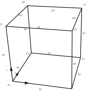
Figure 2.1 Numbering of mesh cell corners and edges . . . 31

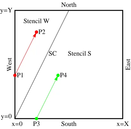
Figure 3.1 Separation of Dby SC in 2D. . . 48

Figure 3.2 Separation of Dby SC and SPs in 3D. . . 50

Figure 3.3 Tracking the SC and SPs. . . 62

Figure 3.4 Tracking of SP. . . 65

Figure 3.5 Tessellation of Type I cells . . . 68

Figure 3.6 Illustration of Lathrop’s test problem. . . 77

Figure 3.7 Centerline flux for Lathrop’s problem. . . 78

Figure 4.1 Exact spatial weights for AHOTN. . . 100

Figure 4.2 Relative error associated with spatial weight for orders Λ = 0,1. . . 102

Figure 4.3 Scaling of Tracking Algorithm. . . 107

Figure 4.4 Decomposition of faces intersected by SP/SC. . . 108

Figure 5.1 Convergence of the AHOTN method of orders one through 3 for theC0(I) test case. . . 115

Figure 5.2 Convergence of the AHOTN method of orders one through 3 for theC1(I) test case. . . 116

Figure 5.3 Convergence of selected other method of orders one and two for theC0(I) test case. . . 117

Figure 5.4 Comparison of continuous k · k_c,ψ,₂ norm and discrete k · k_d,φ,₂ norm of the error for C0(I) test case solved using the complete DGFEM method of order Λ = 1. . . 120

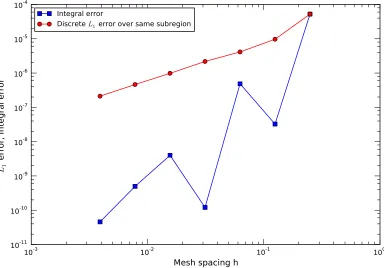
Figure 5.5 Integral error (1/8 subcube) and discrete L1 scalar flux error (for the same region) for test C1(I) solved with the Linear-Linear method. . . 121

Figure 5.6 Comparison of the performance of the SCT method (order Λ = 0) and various other method of order Λ = 1 for the C0(I) test case. . . 123

Figure 5.7 Comparison of the performance of the SCT method (order Λ = 0) and various other method of order Λ = 1 for the C0(II) test case. . . 124

Figure 5.8 Comparison of theL2norm performance of the SCT method (order Λ = 0) and various other method of orders Λ = 1 to Λ = 3 for the C0(II) test case. . . 125

Figure 5.9 Comparison of the performance of the SCT method (order Λ = 0) and various other method of order Λ = 1 for the C1(I) test case. . . 126

(12)

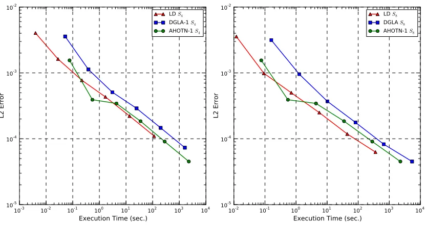
Figure 5.11 DiscreteL2error versus execution time for the LD, DGLA-1, and

AHOTN-1 method for theC1(I) test case. The left subplot containsS4 level

sym-metric results while the right subplot contains results obtained with the

S8 level symmetric quadrature. . . 133

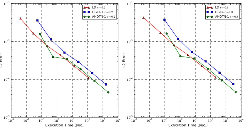
Figure 5.12 DiscreteL2error versus execution time for the LD, DGLA-1, and

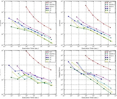
AHOTN-1 methods for the C1(I) (left subplot) andC1(V) (right subplot) test case. 134 Figure 5.13 DiscreteL1 error versus execution time for various spatial discretization

methods for orders for the C1(I) test case. The shaded area is identical

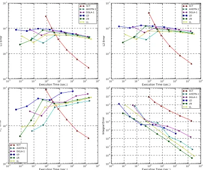
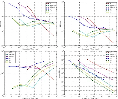
in both plots to facilitate comparison between the two plots. . . 135 Figure 5.14 DiscreteL2 error versus execution time for various spatial discretization

in both plots to facilitate comparison between the two plots. . . 135 Figure 5.15 DiscreteL∞error versus execution time for various spatial discretization

in both plots to facilitate comparison between the two plots. . . 136 Figure 5.16 Integral error norm (computed for the left lower eighth subcube) versus

execution time for various spatial discretization methods and orders for theC1(I) test case. The shaded area is identical in both plots to facilitate comparison between the two plots. . . 136 Figure 5.17 ContinuousL2 error versus execution time for various spatial

discretiza-tion methods for orders for the C1(I) test cases. . . 137 Figure 5.18 DiscreteL2 error versus execution time for various spatial discretization

methods and orders for theC1(II) test case. The shaded area is identical

methods and orders for theC1(III) test case. The shaded area is identical

methods and orders for theC1(IV) test case. The shaded area is identical

in both plots to facilitate comparison between the two plots. . . 143 Figure 5.21 Illustration of the process that leads to broad maxima in the error versus

execution time/mesh spacing curves. Cases γ << 1, γ ≈1 and γ >> 1 are snapshots of scenarios corresponding to an under-resolved solution with small error, poorly resolved solution with large discretization error (maximum of error) and well resolved solution with small error, respec-tively. . . 146 Figure 5.22 Discrete and ContinuousL2error norm results for test casesC1(I) through

C1(IV) obtained using the DGLA-1 method. . . 147

Figure 5.23 Integral error norm versus execution time for various spatial discretization methods and orders for theC1(II) test case. The shaded area is identical in both plots to facilitate comparison between the two plots. . . 148 Figure 5.24 Integral error norm versus execution time for various spatial discretization

(13)

Figure 5.25 Integral error versus execution time for various spatial discretization meth-ods and orders for the C1(IV) test case. The shaded area is identical in

both plots to facilitate comparison between the two plots. . . 150 Figure 5.26 Comparison of the model Eq. 5.38 and the DGC-2 error versus execution

time curve for test case C1(II). . . 152

Figure 5.27 DiscreteL2error norm versus execution time for various spatial discretiza-tion methods and orders for the C1(VI) test case. The shaded area is

identical in both plots to facilitate comparison between the two plots. . . 153 Figure 5.28 DiscreteL2error norm versus execution time for various spatial

discretiza-tion methods and orders for the C1(VII) test case. The shaded area is

identical in both plots to facilitate comparison between the two plots. . . 154 Figure 5.29 Plot of the importance of mixed flux expansion terms κ versus aspect

ratio parameter δ for expansion orders Λ = 1,2,3. . . 155 Figure 5.30 DiscreteL2error norm versus execution time for various spatial

discretiza-tion methods and orders for theC0(I) test case. Red line indicates neces-sary level of mesh refinement (translated into execution time) from where on standard methods’ results are trustworthy. . . 156 Figure 5.31 DiscreteL2error norm versus execution time for various spatial

discretiza-tion methods and orders for theC0(II) test case. Red line indicates neces-sary level of mesh refinement (translated into execution time) from where on standard methods’ results are trustworthy. . . 156 Figure 5.32 DiscreteL2error norm versus execution time for various spatial

discretiza-tion methods and orders for the C1(VII) test case. Red line indicates

necessary level of mesh refinement (translated into execution time) from where on standard methods’ results are trustworthy. . . 157 Figure 5.33 Integral error norm versus execution time for various spatial discretization

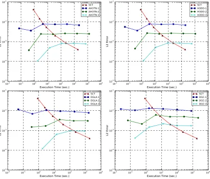
methods and orders for the C0(I) test case. The shaded area is identical in both plots to facilitate comparison between the two plots. . . 158 Figure 5.34 Coupling coefficients ¯cS,F versusσtfor test case I (unity aspect ratio) and

AHOTN, HODD, DGLA, and DGC of orders Λ = 0, ...4. . . 164 Figure 5.35 Coupling coefficients ¯cS,E (East outflow face) versus σt for test case II

(non-unity aspect ratio) and AHOTN, HODD, DGLA, and DGC of orders Λ = 0, ...4. . . 165 Figure 5.36 Coupling coefficients ¯cS,N (North outflow face) versus σt for test case II

(non-unity aspect ratio) and AHOTN, HODD, DGLA, and DGC of orders Λ = 0, ...4. . . 166 Figure 5.37 Coupling coefficients ¯cF,F0 forF =W, S, B andF =E, N, T versusσ_t for

test case II and AHOTN, HODD, DGLA and DGC of order Λ = 0. Note, DGLA and DGC are essentially the same method, the Step Method. . . . 169 Figure 5.38 Coupling coefficients ¯cF,F0 for F = W, S, B and F0 = E, N, T versus σ_t

for test case II and AHOTN, HODD, DGLA and DGC of order Λ = 1. . . 170 Figure 5.39 Coupling coefficients ¯cF,F0 forF =W, S, B andF =E, N, T versusσ_t for

test case II and AHOTN, HODD, DGLA and DGC of order Λ = 2. . . 171 Figure 5.40 Negativity measure τ_ψw versus interpolation order for AHOTN, HODD,

(14)

Figure 5.41 Evolution of negativity measuresτ_ψw andτ_φw with refinement for Lathrop-I-1, Lathrop-ILathrop-I-1, and Lathrop-III-1 test cases. . . 173 Figure 5.42 Negativity measure τ_ψw versus mesh spacing for test case Lathrop-III-1

and various spatial discretization methods. . . 175 Figure 5.43 Negativity measure τ_φw versus mesh spacing for test case Lathrop-III-1

and various spatial discretization methods. . . 175 Figure 5.44 Negativity measure τ_ψw versus mesh spacing for test case Lathrop-III-2

and various spatial discretization methods. . . 177 Figure 5.45 Negativity measure τ_ψw versus mesh spacing for test case Lathrop-III-3

and various spatial discretization methods. . . 177 Figure 5.46 Negativity measureτ_ψw versus scattering ratio for DD solutions with and

without using the first collision source. . . 179 Figure 5.47 Sparsity pattern plot of the HODD-1B matrix. The matrix has full rank. 187 Figure 5.48 Sparsity pattern plot of the DDB matrix. The matrix has full rank. . . . 190 Figure 5.49 Sparsity pattern plot of the AHOTN-1 B matrix. The matrix has rank

485. . . 194 Figure 5.50 Sparsity pattern plot of the LL/LNBmatrix. The matrix has full rank. . 199 Figure 5.51 Results for thick diffusion limit numerical experiment for the LL and

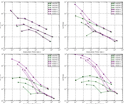
LN method. Neither of these two discretization methods has the thick diffusion limit. . . 200 Figure 5.52 Results for thick diffusion limit numerical experiment for AHOTN of

or-ders zero through three. Except for AHOTN-0, all other methods possess the diffusion limit. . . 202 Figure 5.53 Results for thick diffusion limit numerical experiment for HODD of orders

zero through three. Clearly HODD-0,1,2 do not possess the thick diffusion limit, but for HODD-3 , could not be decreased far enough to make a definite conclusions. . . 203 Figure 5.54 Results for thick diffusion limit numerical experiment for DGLA of

or-ders zero through three. Except for DGLA-0 (Stepmethod), all DGLA methods feature the thick diffusion limit. . . 204 Figure 5.55 Results for thick diffusion limit numerical experiment for DGC of orders

zero through three. None of the DGC orders possesses the thick diffusion limit. . . 205

Figure 6.1 Schematic of the NEA box-in-box benchmark suite. . . 211 Figure 6.2 Penalty functions rl forl= 1,2,3, L and NEA-I test cases for all

consid-ered decision metric’s weights β~. . . 224 Figure 6.3 Penalty functions rl forl= 1,2,3, Land NEA-II test cases for all

consid-ered decision metric’s weights β~. . . 225 Figure 6.4 Penalty functions rl for l = 1,2,3, L and NEA-III test cases for all

con-sidered decision metric’s weights β~. . . 226 Figure 6.5 Penalty functions rl for l = 1,2,3, L and NEA-IV test cases for all

(15)

Figure F.1 Results of the validation exercise for NEA-I withβ~ = (0,0,0,1). . . 317

Figure F.3 Results of the validation exercise for NEA-I withβ~= (1,0,1,0). Quantity 3.c is selected as target quantity. . . 318

Figure F.5 Results of the validation exercise for NEA-II withβ~= (0,0,0,1). . . 319

Figure F.8 Results of the validation exercise for NEA-III withβ~ = (0,0,0,1). . . 320

Figure F.11 Results of the validation exercise for NEA-IV withβ~= (1,0,1,0). . . 322

(16)

Chapter 1

Introduction

Solving particle transport problems is of great interest in many disciplines of science and en-gineering such as nuclear reactor design, astro-physics and health-physics. Traditionally, two

vastly different methods were developed to obtain approximate solutions of transport problems,

namely stochastic methods (typically referred to as Monte Carlo methods) and deterministic methods; only the latter shall be of interest in this work.

Common to all deterministic algorithms that approximate solutions to transport problems

is that they attempt to solve some form of the linear particle transport equation. The two most prominent forms of the linear transport equation are the integro-differential and the integral

forms[2], both of which find wide application as the starting point for the derivation of numerical

solution methods, but only the former will be considered in this work.

The primary, dependent variable in a deterministic transport calculation is the angular flux,

which depends on the six independent phase space variables space and velocity1, and, possibly the time variable as well. In order to obtain a system of equations that can be solved on a digital computer, all these variables have to be discretized. Because of the lack of alternatives,

the energy variable is almost invariably discretized via the multigroup formalism[3], which

integrates the transport equation separately over a finite number of energy bins and defines multigroup constants that conserve relevant quantities, e.g. reaction rates, integrated over each

energy bin.

For the discretization of the directional variable, two main flavors have developed over the course of the years, namely the SN and the PN methods. The SN method is a collocation method in angle first introduced in [4], while thePN[5] method projects the transport equation onto the orthogonal set of spherical harmonics[6] that is appropriately truncated, thus closing the resulting system of equations. Throughout this work the SN method is adopted. Within the framework of this thesis, we are concerned with the discretization of theSN equations which

(17)

are a set of linear hyperbolic equations in space. The discretization of the spatial variable of the

SN equations will be referred to as spatial discretization. Therefore, the exact solution of the

SN equations is considered the reference solution for all the following discussion. This means that the discussion is confined to the multigroup-SN realm.

In contrast to the discretization in angle and energy, numerous schemes have been pro-posed for the discretization of the spatial variables, particularly for the multigroup SN equa-tions comprising classical finite difference methods, finite volume methods, short characteristic

methods, nodal methods and discontinuous finite element methods. This work will elaborate on the relationships between some of these broad classes of methods. The abundance of spatial

discretization methods can be attributed to the plethora of typical requirements for the

dis-cretization methods. Often, the prospective user has a list of properties ranked from essential to important to nice-to-have. This “check-list” is highly application specific and will therefore

vary significantly by application and purpose of the calculation. In the following, a list of

possible properties that users might require from spatial discretization methods is compiled:

A. Essential Properties Required of SN Discretization:

1. Conservation of neutrons: The discretization method satisfies a discrete version of the balance equation.

2. Algebraic linearity: The discretization method does not introduce non-linearities

into the underlying numerical method equation or the iterative solution process.

B. Important Properties Required of SN Discretization:

1. Accuracy: Given a fixed mesh size, the method is close to the exact solution in a

norm relevant to the user.

2. Second order truncation error: Assuming a sufficient number of partial derivatives

is bounded, the method features a truncation error larger than unity.

3. Pointwise/cellwise convergence: The numerical solution converges to the true

solu-tion everywhere even if the exact solusolu-tion is non-smooth.

4. Resolution of the diffusion limit: In the thick diffusion limit the discretization of the

SN equations satisfies, to leading order, a discretization of the Diffusion equation. 5. Execution time: Given a fixed mesh size and spatial expansion order (collectively

described by the number of degrees of freedom), the execution time of the method is small.

6. Computational efficiency: Refers to how much execution time is necessary to achieve

(18)

7. Positivity: Given a positive source and positive inflow into a mesh cell, the

dis-cretization method does not produce (or is less susceptible to producing) unphysical negative cell-averaged and cell face angular fluxes.

C. Desirable Properties of SN Discretization:

1. Robustness: No unphysical oscillations are present even in the presence of strong material heterogeneities, voids, and the like.

2. Minimal spreading of a beam in vacuum (numerical diffusion).

The above list of desired properties is partially adapted from [7] and [8], but it is by no means

complete. The properties in A are satisfied by all methods considered in this work (i.e. all methods are conservative and algebraically linear), and are therefore not discussed in any

detail. Subset B is within the main focus of this work, while subset C is beyond the scope of

this work.

The coexistence of a multitude of spatial discretization schemes is due to the lack of a

consistent best performer according to these measures among the set of available schemes.

In addition, some of the listed properties are mutually exclusive, e.g. A.2, B.2, and B.7: Algebraically linear, second order methods that preclude negative fluxes cannot exist[9]. The

choice of a suitable discretization method is driven by the needs of the user and thus the

characteristics of the specific problem to be solved.

This work is concerned with investigating the performance of various spatial discretization

schemes of the one-group, multidimensional SN equations on Cartesian grids with respect to the properties listed above to guide the decision making process in real world applications. To

this end three sets of test problems are employed to evaluate the performance of a selection

of spatial discretization methods and rank their performance based on suitable performance metrics. A fitness function, adjustable to a given “check-list” of requirements, is designed that

aggregates the data obtained from these test problems into a single number indicating how

suitable a discretization method is for a specific problem. The fitness function explicitly allows for augmenting the current set with new properties that are not considered within this work,

for example robustness in the presence of strong material heterogeneities and/or voids.

The four properties that this work focuses on are execution time, accuracy, positivity, and possession of the discrete diffusion limit; accuracy and execution time, are frequently aggregated

into the method’s computational efficiency.

Three test problems are used to characterize the performance of the considered discretization methods with respect to the selection of desired properties. This work’s results are based on

the assumption that the data obtained from the test cases are representative of more complex,

(19)

A set of pre-existing, promising discretization methods was selected, including discontinuous

finite element methods (DGFEM) ([10], [11], [12]), the simple corner balance method (SCB) [7], AHOTN methods[13], linear-nodal(LN), and linear-linear (LL) methods[14] and the arbitrary

polynomial order extensions of the Diamond Difference method (HODD) ([15], [16]). All were

implemented for three-dimensional Cartesian geometry.

In addition, a novel method that explicitly tracks and eliminates lines and planes of

non-smoothness originating from “inconsistent” boundary conditions was developed and

imple-mented. This method uses the Step approximation in all cells that are intersected by lines and planes of non-smoothness. It can be considered an extension of Duo’sSingular

Character-istic Trackingalgorithm[17] to three spatial coordinates. However, it is important to point out

that this extension is highly non-trivial because of the tremendous increase in complexity of the tracking and cell-splitting algorithms involved. The new method is labeled SCT-Stepmethod.

All implementations place a high premium on reducing the computational overhead to a

minimum in order to level the playing field for a fair comparison with respect to the efficiency aspect discussed before. In addition to implementing these methods, analysis was performed

showing that several classes of methods can be recast as discontinuous finite element methods

thus unifying the treatment of methods that we previously thought to be unrelated.

The test problems presented within this work are utilized to measure the performance of

the implemented spatial discretization methods. The first set of test problems focuses on mea-suring the discretization method’s accuracy and execution time. It is based on an extension

of Larsen’s two-dimensional homogeneous square test[18] to three spatial dimensions and

scat-tering media. This is achieved by utilizing the Method of Manufactured Solution (MMS) [19] approach which allows for securing knowledge of the underlying exact solution without

com-promising the necessary complexity of the test problem. In contrast to slab geometry, realistic

multi-dimensional SN problems support at most bounded first order partial derivatives of the angular flux[20] thus limiting the attainable convergence rate (with mesh refinement) of any

standard spatial discretization method. Therefore, viable test cases need to take the limited

exact solution smoothness into consideration because it directly affects the solution accuracy of deployed spatial discretization methods ([21], [22], [17]). The implemented three-dimensional

MMS test suite explicitly accommodates an arbitrary degree of smoothness of the exact

under-lying solution.

The second family of test problems is based in Lathrop’s test case [9]. It is designed to be

a challenging test for methods’ resilience against negative fluxes. It consists of a small source

region (region I) enclosed in a large, typically optically thick, source-free region (region II). The solution in region II often suffers from the occurrence of negative fluxes. A family of test

problems is created by varying the total cross sections and scattering ratios of the involved

(20)

Finally, the third problem tests whether the selected methods possess the thick diffusion

limit. Consider a configuration with the property that the optical thickness increases while particle removal, absorption and leakage across the boundaries, vanishes. In this configuration,

a typical length scale over which the flux changes significantly is not determined by the

parti-cle’s mean free path but by the (much larger) diffusion length. Therefore, sufficiently accurate results can be obtained on very coarse meshes (with respect to the particles mean free path) if

the method possesses the diffusion limit. A method is said to possess the diffusion limit if the

corresponding discretization limits to a discretization of the diffusion equation in configurations as described above. The third set of challenge problems features a homogeneous medium with

vacuum boundary conditions on all outside boundaries. The material properties are subjected

to scaling using a small parameter such that in the limit of small values, the problem approaches the diffusion limit. The methods’ solutions are then compared to the limiting solution of the

dif-fusion problem. For a selection of discretization methods, analysis was performed corroborating

the results of the thick-diffusion test problem.

The final goal of this work is the construction of a performance metric aggregating data

measuring vastly different properties of the selected discretization methods. The approach

taken within this work computes a single fitness value for spatial discretization methods based on user-selected properties that are ranked by importance to the user. The fitness value has

the property that it ranges from zero to unity, with zero being the worst and unity being the best score.

This metric, once validated, would be of great utility in production-level SN codes where the user would set their requirements as input to the code then the decision metric would automatically choose among the various discretization methods implemented in the code that

best suits the user’s demands.

1.1 The Transport Equation

The linear Boltzmann transport equation describes the evolution of the flux of neutral particles,

i.e. neutrons or photons, in a host medium. It can be obtained from the general Boltzmann

transport equation by neglecting particle-particle interactions, the dependence of the material properties of the host medium on the particle flux, and assuming that no electric force field is

present. Heuristically, it can be derived as a detailed balance of particle production and loss

(21)

initial conditions in a form that is general enough for our purposes is given by:

1

v ∂ψ

∂t + ˆΩ· ∇ψ+σt(~r, E, t)ψ(~r,

ˆ

Ω, E, t) =

Z

4π

dΩˆ0

Z ∞

0

dE0σs(~r,Ωˆ·Ωˆ0, E0 →E, t)ψ(~r,Ωˆ0, E0, t)+

κ(E) 4π

Z

4π

dΩˆ0

Z ∞

0

dE0ν(~r, E0, t)σf(~r, E0, t)ψ(~r,Ωˆ0, E0, t) +

q(~r, E, t)

4π if~r∈D ψ(~r,Ωˆ, E,0) = ψ0(~r,Ωˆ, E)

ψ(~r,Ωˆ, E, t) = ψB(~r,Ωˆ, E, t) if~r∈∂Dand ˆn·Ωˆ <0, (1.1)

where

• ~r= (x, y, z)T: Vector of Cartesian spatial coordinates

• Ω = (ˆ µ, η, ξ)T: Unit vector of direction cosines with respect to coordinate axesx,y and

z.

• E: Energy.

• t: Time.

• ψ(~r,Ωˆ, E, t): Angular flux.

• σs(~r,Ωˆ ·Ωˆ0, E0 →E, t): Double differential, macroscopic scattering cross section.

• σt(~r, E, t), σf(~r, E, t): Macroscopic total collision and fission cross section, respectively.

• κ(E): Fission spectrum.

• ν: Fission yield.

• q(~r, E, t): Isotropic external distributed source.

• ψ0(~r,Ωˆ, E): Initial condition: known flux att= 0.

• ψB(~r,Ωˆ, E, t): Explicit boundary conditions: known incoming flux on the boundary.

• nˆ: Outward normal vector defined on the boundary∂D.

The independent variables ~r, ˆΩ, and E constitute the six-dimensional phase space, and the dependent variable, the angular flux ψ, is a distribution over the independent variables.

In this work we are only concerned with steady state solutions of the one-group transport

(22)

of the angular flux with respect to time is set to zero, and the time arguments are dropped in the

angular flux and the cross sections. Further, as the medium is non-multiplying and scattering is isotropic: σf = 0 andσs(~r,Ωˆ·Ωˆ0, E0→E) =σs(~r, E0 →E)/4π. Thus the transport equation can be written as:

ˆ

Ω· ∇ψ+σt(~r, E)ψ(~r,Ωˆ, E) = 1 4π

Z ∞

0

dE0σs(~r, E0 →E)φ(~r, E0) +

q(~r, E)

4π for~r ∈D, (1.2)

where the scalar fluxφhas been introduced:

φ(~r, E) =

Z

4π

dΩˆψ(~r,Ωˆ, E). (1.3)

For the purpose of discretizing the energy variable, we apply the operator R∞

0 dE· to the

continuous-energy transport equation, Eq. 1.2, using the following definitions:

ˆ

ψ(~r,Ω)ˆ =

Z ∞

0

dEψ(~r,Ωˆ, E) ˆ

φ(~r) =

Z ∞

0

dEφ(~r, E)

σs(~r, E0) =

Z ∞

0

dEσs(~r, E0 →E)

ˆ

σk(~r) =

R∞

0 dEσk(~r, E)ψ(~r,Ωˆ, E)

ˆ

ψ fork=t, s

ˆ

q(~r) =

Z ∞

0

dEq(~r, E),

Using these expressions, Eq. 1.2 can be rewritten as

ˆ

Ω· ∇ψˆ+ ˆσt(~r) ˆψ(~r,Ω) =ˆ 1

4πσˆs(~r) ˆφ(~r) +

ˆ

q(~r)

4π for~r ∈D. (1.4)

For the sake of convenience we omit the hat above all quantities in the remainder of the

discussion.

The one-group transport equation, Eq. 1.4, depends continuously on the five remaining phase space variables, namely space ~r, and direction of motion of the particles ˆΩ. As this work is concerned with the spatial discretization in particular, we discretize the directional

variable via theSN method and use the resulting equations as the starting point of all further discussions. TheSN method proceeds by solving the transport equation only along discrete rays

ˆ

Ωn= (µn, ηn, ξn)T, with n= 1, .., N, approximating the integration over the angular variables by a quadrature rule {Ωˆn, wn}n=1,..,N satisfying

N

P

n=1

(23)

Eq. 1.4 yields:

ˆ

Ωn· ∇ψn+σt(~r)ψn(~r) = 1

4πσs(~r)φN(~r) + q(~r)

4π forn= 1, .., N and~r ∈D φN(~r) =

N

X

n=1

wnψn(~r)

ψn(~r) = ψB(~r,Ωˆn) for n= 1, .., N and~r ∈∂Dand ˆn·Ωˆ <0, (1.5)

whereψn(~r)≈ψ(~r,Ωˆn) is an approximation of the true one-group angular flux at ˆΩn.

The set ofSN equations Eq. 1.5 continuously depends on the spatial variables~r = (x, y, z)T. All comparisons between reference and numerical solution is made within the SN framework, i.e. the reference as well as the numerical solution both adopt the SN approximation for the discretization of the angular variables. Consequently, discretization errors are entirely due to

the applied spatial discretization and not due to the finite number of utilized discrete directions

N.

1.2 Solution of the One-Group

S

N

Equations

This section briefly introduces methods to iteratively solve the one-groupSN equations in their first order form. As this work is concerned with spatial discretization methods and not with the

iterative solution of theSN equations, this section shall not aspire for completeness, but rather introduce the concept of the space-angle mesh sweep, the source iteration, and the GMRES solution of the SN equations to the unfamiliar reader.

1.2.1 Space-Angle Mesh Sweep

Let us first discuss the solution of the SN equations in the absence of scattering leading to a set of decoupled first order partial differential equations:

ˆ

Ωn· ∇ψn+σt(~r)ψn(~r) =

q(~r)

4π forn= 1, .., N and ~r∈D φN(~r) =

N

X

n=1

wnψn(~r). (1.6)

Anticipating the detailed discussion of spatial discretization schemes, the solution of a single

SN equation along directionnwith a given source term can be accomplished by using a mesh sweep[23] if the discretization uses only information from upstream cells. A mesh sweep starts in

(24)

including the face fluxes separating this cell and its downstream neighbors, the next downstream

cell can be solved by using the already obtained solution for the corner. By repeating this basic step, the spatial mesh can be swept in the downstream direction for each ˆΩn until the solution

in all cells is obtained.

Mathematically, the mesh sweep recognizes that the global system of discretized equations for each direction ˆΩn, i.e. the algebraic system comprising the streaming and total interaction

operators, is lower or upper triangular (depending of the numbering of the unknowns), and the

mesh sweep resembles forward or backward substitution, respectively.

Performing mesh sweeps for all directions in the quadrature set (n= 1, ..., N) and applying the quadrature formula completes a single space-angle sweep. If the considered problem is

in fact non-scattering, a single space-angle mesh sweep returns the full solution of the SN equations. In the presence of scattering, an iterative algorithm is necessary for obtaining the

solution of the SN equations.

1.2.2 Source Iterations

The right hand side of the SN equations, Eq. 1.5, comprises the weighted sum of the angular fluxes along all directions, thus coupling the equations across discrete ordinates. Typically, for

the sake of performance, the solution of the SN equations progresses one discrete ordinate at a time via a space-angle sweep such that a viable iteration scheme must decouple the discrete

ordinates within iterations. The idea of the predominantly usedSource Iteration method is to

guess the angular flux, compute the scattering source and right hand side of Eq. 1.5, compute the angular fluxes for all n = 1, ..., N using a space-angle sweep, and then recompute the scattering source. Formally, this can be written as

ˆ

Ωn· ∇ψpn+1+σt(~r)ψpn+1(~r) = 1

4πσs(~r)φ

p N(~r) +

q(~r) 4π φp_N+1(~r) =

N

X

n=1

wnψnp+1(~r), (1.7)

wherep is the iteration index. Switching to more convenient operator notation borrowed from [24], Eq. 1.7 is recast as:

ψ_np+1 =L−1(Sφp+q)

φp+1 =Dψp+1. (1.8)

where L, S, and D are the streaming/collision, scattering, and quadrature operators,

respec-tively. It is understood that the streaming/collision operator is inverted matrix-free within the

(25)

1.2.3 GMRES Solution of SN equations

Recently, attention has arisen to utilize the Generalized Minimal Residual (GMRES)[25] solver

for the solution of the one-group SN equations. The specifics of the GMRES method are detailed in [25]. Here, it shall be sufficient to mention that GMRES only requires matrix-vector multiplications of a matrixAto solve the linear systemAx=b. Within theSN setting, GMRES is utilized as follows[24]. First Eq. 1.8 is manipulated to obtain

Dψn=φ=DL−1(Sφ+q)⇒



I−DL−1S | {z }

A 

φ=DL−1q, (1.9)

where iteration indices are dropped. Then, it is recognized that only the matrix-vector product

involvingA is required. Therefore, the solution of theSN equations uses four simple steps: Before starting GMRES iterations:

0. Perform a single space-angle sweep on the fixed source b = DL−1q to obtain the right-hand side for GMRES solution.

Matrix Vector Product: (I−A)v

1. Compute the scattering source s=Sv.

2. Space-angle sweep on the scattering source v0 =DL−1_s_.

3. Return v−v0.

Given an implementation of the source iteration scheme it is straight forward to implement a

GMRES solver subroutine because it relies on the same basic functions that are instrumental

to source iterations.

1.3 Thesis Outline

This thesis is organized as follows: in chapter 2 all contending discretization methods are re-viewed. It is demonstrated that several of these methods can be recast as discontinuous

finite-element methods thus creating a common framework of related methods. Subsequently, the

utilized test cases are introduced in chapter 3. The implementation of the contending methods along with two new algorithms regarding spatial discretization methods of theSN equations are discussed in chapter 4. In chapter 5 numerical results of the contending discretization methods

(26)

obtained from the “numerical experiments” in chapter 5 serves as the basis of the

(27)

Chapter 2

Review of Spatial Discretization

Methods

It is the purpose of this work to compare the properties of various (promising) spatial

discretiza-tion methods of the multi-dimensional SN equations. This chapter introduces a general clas-sification of spatial discretization methods especially stressing the importance of discontinuous finite element methods (DFEM) before laying out the general framework typically used for the

derivation for these methods. Subsequently, methods traditionally used for the discretization of theSN equations are reviewed along with accounts of their performance whenever available. Finally, some of the reviewed methods are re-derived as DFEM methods, thus reducing the

difference between them to differences in the respective test and trial spaces.

2.1 General Classification of Spatial Discretization Methods

The ultimate goal of this work is to construct a decision metric associating features of a given test

problem and the computed quantities of interest with the best performing spatial discretization scheme. To this end, it is useful to elaborate on the classification of spatial discretization

schemes typically encountered in computational science. Moreover, terminology in most fields

like computational fluid dynamics (CFD) closely follows the standard jargon, but computational neutron transport methods evolved without much communication with other fields, and thus

utilize a slightly different terminology. This section contrasts three broad classes of spatial discretization methods, namely finite difference methods (FDM)[26], finite volume methods

(FVM)[27], and finite element methods (FEM)[28]. It also classifies the type of schemes that

are considered in the remainder of this work in the standard jargon as used in [10].

The FDM approximates the solution of the constituting PDEs by grid function values that

(28)

PDE by finite differences. Since finite differences involve the grid function value at neighboring

points the equation obtained at each grid point is coupled to the equations at a certain number of neighboring grid points. The approximation order of a finite difference scheme is determined

by the employed finite differences: The more neighboring points are involved, the higher in

general the order of accuracy1, but the more coupling between the equations.

In this work, FDMs are not considered for two reasons: First, the SN equations are an expression of neutron balance, but the FDM is in general not conservative because it

approx-imates the neutron flux at grid points as opposed to over cell volumes. Second, the coupling between neighboring grid points necessitates solving a global matrix equation involving all grid

function values if the finite differences involve downstream as well as upstream information. If

only upstream values2 are utilized, sweeping the mesh is still possible. However, depending on the size of the finite difference stencil, a memory overhead compared to more localized methods

can be expected because the global system of equations has more non-zero off-diagonal terms.

An additional problem when using wide stencils is how to generate grid function values out-side of the domain which are necessary when evaluating the FDM equations for points close to

the boundary. Further shortcomings of the FDM are that it cannot be extended to

unstruc-tured grids (such as tetrahedral grids) and that it may exhibit oscillations near sharp material discontinuities because of the near-discontinuous[29] underlying solution in their vicinity. For

the reasons mentioned above, the FDM method is currently not used in neutron transport applications any more, but older attempts can be found in [20].

The FVM most often used in CFD decomposes the domain into homogeneous mesh cells,

then integrates the system of conservation equations over the extent of each cell. Subsequently, Gauss’ theorem is used and the volume integrals of the derivative terms are recast as integrals

over the cell faces. Using the homogeneity of the cell, the volume and face integrals can then

be rewritten as averages of the dependent variable over the volume and faces, respectively. In the framework of FVMs, the face-averaged fluxes that originate from applying Gauss’ theorem

are referred to as numerical fluxes.

The obtained balance-relation between the numerical fluxes and the average is exact, but it comprises more unknowns than equations, and hence requires closure. The closure is usually

obtained via a reconstruction approach, which assumes that the true dependent variable has

the shape given by some simple function, e.g. a polynomial of some order. Using the averages of the dependent variable in the neighboring cells, an interpolation formula can be devised that

allows for the numerical fluxes on the edges to be computed from the cell averages living in the

neighboring cells[27].

However, the interpolation formula also globally couples the averages in neighboring cells

1

Given sufficient smoothness of the underlying exact solution.

(29)

in a manner very similar to FDM (with the exception of the first order step method), imposing

the restriction that increasing the accuracy requires enlarging the stencil, thus causing more coupling between cells. Moreover, if the interpolation formula requires downstream values, then

the full global system of equations has to be solved simultaneously, increasing the execution time

tremendously. Finally, if sharp material discontinuities exist, then the solution might feature oscillations because the reconstruction spanning multiple cells assumes that the underlying

solution does not stray too much from the assumed polynomial shape.

Common to all FEM schemes is that the solution of the PDE is approximated by a linear combination of functions belonging to some finite dimensional trial function space. The

un-knowns of the FEM computation are the coefficients of the linear combination of trial functions,

also referred to as expansion coefficients. Several different approaches exist to derive an alge-braic system of equations for the unknown expansion coefficients, but common to all of them

is that the set of PDEs is replaced by an integral formulation of the problem, i.e. the set of

equations of interest is replaced by some integral over the domain of interest: If the solution of the PDE minimizes a particular functional, then the flux expansion via the trial functions

can be substituted into the functional, and setting the functional’s derivatives with respect to

the expansion coefficients to zero provides enough equations to determine all expansion coeffi-cients (Ritz method). If such a functional does not exist, then the residual of the approximate

solution can be required to be orthogonal to a set of test functions with respect to some in-ner product(weighted-residual method). Finally, the least squares FEM (LSFEM) requires the

integral of the square of the residuals over the domain to be minimal.

The FEMs can further be divided into continuous (CFEM) and discontinuous methods (DFEM), with the difference between these two classes being whether the global approximate

solution is continuous or not. Continuity in an FEM scheme is generally enforced by letting test

and trial function spaces be supported on adjacent patches of cells such that flux values at the interfaces of cells are unique, i.e. regardless from which cell the interface point is approached,

the same flux value is encountered.

The flux shape on the interfaces can be retrieved by the unique (polynomial) interpolation through the flux values on the interface. As the flux values on the interfaces are unique, the

polynomial interpolation is also unique and therefore the flux is continuous pointwise on the

interface. On the other hand DFEMs restrict the support for test and trial functions to a single cell such that flux values at the interfaces are local to one cell and therefore not unique[10].

The coupling across cell interfaces in DFEMs is achieved by imposing boundary conditions on

the cells faces only in an integral (as opposed to pointwise) sense, which is very similar to the way FVMs impose cell boundary conditions.

From an algorithmic point of view, the major difference between CFEM and DFEM is that

(30)

exhibits a block structure arising from the local character of the test and trial function spaces

with very little interdependency between the blocks. As a consequence, CFEM necessitates the simultaneous solution of the global system of equations, but DFEM might allow a mesh

sweep if information only propagates downstream. At each step of this mesh sweep, a local

system of equations has to be solved whose size depends on the local expansion order but is typically much smaller than the global system of equations. The preferential propagation of

information in the SN equations is accounted for by using the numerical upstream flux which allows application of the mesh sweep, while for CFEMs the preferential direction cannot be accounted for, leading to stability problems.

In summary, the FDM, FVM, and CFEM in their typical form all exhibit undesirable

properties that render them unfit for the solution of theSN equations, while the broad class of DFEM is well suited for this purpose. Consistent with Ref. [10], the general scope of methods

considered in this work is referred to as nodal methods, which is used synonymously with

DFEM. Nodal methods are a class of methods that share the following properties:

• All function spaces are defined local to a mesh cell.

• Coupling between cells occurs only through their faces.

• Coupling between cells is only imposed in an integral sense.

• Increasing the order of the methods is achieved by increasing thelocalorder of expansion.

In neutron transport theory, various spatial discretization methods have been derived using

physical arguments, but the final methods still shared all properties of nodal methods. The term nodal method in neutron transport theory strictly applies to methods that use a set of

spatial Legendre-Polynomial moments of the SN transport equations augmented by closure relations obtained from transverse moments of the continuum transport equation as e.g. in [13]. Along the same line of thought are short characteristic schemes[30], which use the same

set of moments of the SN equations, but derive closure relations from approximate solutions obtained from the characteristic form of the transport equation.

Both the nodal and characteristic schemes are shown to resemble discontinuous

Petrov-Galerkin FEMs (DPGFEM), and hence fall into the class of nodal methods as defined in this

work([1] and [31]). Discontinuous Petrov-Galerkin FEMs are DFEM, but in contrast to dis-continuous Galerkin methods, they utilize different test and trial spaces while DGFEM utilize

identical test and trial spaces. Many similar schemes exist that utilize the same set of moment

(31)

2.2 Discontinuous Finite Element Framework

Throughout the remainder of this work, the discretization of the spatial variables via the

dis-continuous finite element framework is of special importance. Therefore, this section introduces notation and the weak and strong forms of theSN transport equation that commonly serve as the starting point for the derivation of discontinuous finite element methods.

Let the domain D be decomposed into a set of conforming (no “hanging” nodes) cuboidal elementsQ_~i= [xi−1, xi]×[yj−1, yj]×[zk−1, zk] withxi,yj andzkindicating mesh cell boundaries such that D=S

~i

Q~i and~i = (i, j, k)T. Let the set of all faces in Dbe given by E, and the set of all faces of Q_~i be denoted by

E~i=

n

EN

~i ,E~iS,E~iW,E~iE,E~iT,E~iB

o ,

where N, S, W, E, T, and B represent the north, south, west, east, top and bottom faces, respectively. Associated with each face is a unit outward normal vector ˆnF with F =N, S, W,

E, T, B.

Deviating from standard notation, the E, N, and T faces are always outflow faces, while the W, S, and B faces are always inflow faces. Hence, if components of ˆΩ change sign, then for a given cell the denotation of the cell faces changes. The set of faces is then divided into

inflow and outflow faces according to the sign of the inner product: ˆnF ·Ωˆ <0 and ˆnF ·Ωˆ >0 for inflow and outflow faces, respectively. We refer to the set of all inflow faces as EI, and to

the set of all outflow faces as EO:

EO ₌ _{_EE_,_EN_,_ET_}

EI ₌ _{_EW_,_ES_,_EB_}_. _(2.1)

Further, we associate with each face an interior and exterior trace denoted by EF,+ and EF,−_{, respectively. Restriction of information from within the cell to any face is defined on} the interior trace, while information from outside the cell is restricted to the exterior trace. Note that discontinuities typical for discontinuous finite element methods[10] originate from

the pointwise difference of the exterior and interior flux traces, while for continuous FEM the

interior and exterior traces are identical.

The mesh shall always be constructed to approximate the problem configuration such that

the material properties, i.e. the total cross sectionσt(~r) and the scattering cross sectionσs(~r), are constant within the cell Q_~i; then we denote the total and scattering cross sections within that cell byσ~i_t and σ~i_s, respectively.

(32)

combination of trial functions f~i_n,l(~r):

~r∈Q_~i : ψn(~r)≈ψh,~in (~r) = L

X

l=1

a~i_n,lf~i_n,l(~r), (2.2)

where the expansion coefficients a~i_n,l as well as the trial functions f~i_n,l(~r) may depend on the Discrete Ordinate index n. The superscript h refers to the utilized mesh spacing h = max

~i (xi−xi−1, yj−yj−1, zk−zk−1) and serves as a reminder that the superscripted quantity is an approximation of the exact solution. The global approximation of the angular flux can be

retrieved from the local approximations as their direct sum:

ψ_nh(~r) =M ~i

ψ_nh,~i(~r). (2.3)

Frequently, the restriction of the flux expansion on the cell faces will be needed, so for

convenience we denote the restriction onto the interior trace as:

ψh_n(~r)

_EF,+

~i

= lim →0ψ

h

n(~r+sF||Ω) ifˆ ~r∈E_~iF,

and onto the exterior trace as:

ψh_n(~r)

EF,−

~_i

= lim →0ψ

h

n(~r−sF||Ω) ifˆ ~r∈E_~iF,

where

sF =

(

1 ifF ∈EI

−1 ifF ∈EO_. .

Note, that for the definitions of the restriction operators, the global flux solution is used, which means that the restriction onto the exterior trace uses the flux solution in the appropriate

adjacent cell.

The local space of test functions V~i = span{v~i_l(~r)}L

l=1 with L = Λ3 is defined such that v~i_l(~r) = 0 if~r /∈Q_~i, and as a direct consequence this implies

Z

DdV v

~i

l(~r)G(~r) =

Z

Q~i

dV v~i_l(~r)G(~r) (2.4)

(33)

define

Z

DdV v

~i

l(~r)G(~r) =

v~i_r(~r), G(~r)

D (2.5)

Z

Q~i

dV v~i_l(~r)G(~r) =

v~i_r(~r), G(~r)

, (2.6)

respectively, and similarly for integrals over the cell faces:

Z

EF ~i

dSv~i_l(~r)G(~r) =hv~i_r(~r), G(~r)iF.

2.2.1 The Weak and Strong Form of the SN Transport Equation

The derivation of the weak and strong form of theSN equations largely follows Ref. [10], with the distinct difference that in this work theSN equations are discussed while [10] illustrates the development of the weak and strong form on the basis of the linear one-dimensional transport

equation.

Let the residual of the one-group SN equations, Eqs. 1.5, be given by:

Rn[Gn(~r)] = ˆΩn· ∇Gn(~r) +σt(~r)Gn(~r)−

σs(~r) 4π

N

X

n=1

wnGn(~r)−

q(~r)

4π , (2.7)

with the obvious property that:

Rn[ψn(~r)] = 0.

In order to derive the weak and subsequently the strong form of the within-groupSN transport equation the local approximation of the angular flux in terms of the trial functions ψ_nh is substituted into the expression for the residual Eq. 2.7. Note that now:

Rn

h ψ_nh(~r)

i

6

= 0,

i.e. theSN equations are not satisfied pointwise by ψnh(~r).

However, for deriving a discretized system of equations the residual is required to be

or-thogonal to all members of the test space with respect to the inner product (·,·)_D s.t. by using Eq. 2.4 the following expression can be obtained:

v~i_l(~r),Ωˆn· ∇ψh,~in +σ~itψh,~in (~r)−

σ~i_s

4πφ

h,~i N (~r)−

q(~r) 4π

!

D

(34)

Applying integration by parts to the gradient term results in

−ψ_nh,~i,Ωˆn· ∇v~il

D+ v

~i l(~r), σ

~i

tψh,~in (~r)−

σ~i_s

4πφ

h,~i N (~r)−

q(~r) 4π

!

D

=−X

F

D

v~i_l,nˆT_FΩˆnF∗

E

F , (2.9)

whereF∗ is the numerical flux on the cell faces. The numerical flux is instrumental in coupling the equations on Q_~i to the rest of the domain, i.e. it imposes cell boundary conditions and

controls the flow of information for the discretization method. Equation 2.9 is referred to as

the weak form of the SN equations because it does not require the trial functions (and hence

ψh,~in ) to possess integrable first partial derivatives.

The strong form of theSN equations can be obtained by applying integration by parts again leading to:

v~i_l(~r),Ωˆn· ∇ψnh,~i+σ~itψh,~in (~r)−

σ~i_s

4πφ

h,~i N (~r)−

q(~r) 4π ! D =X F *

v~i_l,ˆnT_FΩˆn ψnh

EF,+

~i

−F∗_F !+

F

,

(2.10)

which in contrast to the weak form requires the trial functions to possess integrable first partial

derivatives. In this work we solely employ the numerical upstream flux given by:

F∗ ₌

   ψh n

EF,−

~i

ifEF ∈EI

ψ_nh

EF,+

~i

ifEF ∈EO

, (2.11)

i.e. the numerical flux is equal to the cell’s interior trace on all outflow faces, but equal to the

appropriate upstream cell’s flux on all inflow edges. Physically, the numerical upstream flux ensures propagation of information only in the direction of neutron travel.

Upon substitution of Eq. 2.11, the weak and strong form Eqs. 2.8 and 2.10 become

−ψ_nh,~i,Ωˆn· ∇v~il

+ v~i_l(~r), σ~i_tψh,~i_n (~r)− σ

~i s 4πφ

h,~i N (~r)−

q(~r) 4π

!

=−X

EO *

v~i_l,nˆT_FΩˆnψhn

EF,+

~i + F −X EI *

v~i_l,ˆnT_FΩˆnψnh

EF,−

~i +

F

, (2.12)

and

v~i_l(~r),Ωˆn· ∇ψnh,~i+σ~itψnh,~i(~r)−

σ~i_s

4πφ

h,~i N (~r)−

q(~r) 4π ! = X EI D

vl,nˆTFΩˆn[[ψhn]]F

E

(35)

respectively, where we defined the jump operator [[]]F as the pointwise difference between the

interior and exterior traces:

[[G(~r)]]F = G|_EF,+− G|_EF,−.

Most of the spatial discretization methods that are discussed in this work can be obtained by selecting appropriate test and trial function spaces which are substituted into the weak

or strong form Eqs. 2.12 and 2.13, respectively, which leads to a local system of algebraic

equations.

2.3 Review of Spatial Discretization Methods for the

S

N

Equa-tions

In this section we review promising classes of spatial discretization schemes including diamond difference type methods, discontinuous Galerkin finite element type methods (DGFEM) and

transverse moments based methods (TMB). For convenience let the spatial Legendre moment

of the flux denoted by ψ~i_{n, ~}_m be defined as:

ψ~i_{n, ~}_m = M_m~i_~ {ψn(~r)}

M~i_m_~ {·} = 1

V~i Z

V~i

dV p~i_m_~ (~r)· , (2.14)

wherem~ = (mx, my, mz)T denotes the order of the moments. Further, triple sums and products of Legendre polynomials are abbreviated by:

Λ X

~ m=0

· =

Λ X

mx=0 Λ X

my=0 Λ X

mz=0 ·

p~i_m_~ (~r) = pi_m_x(x)pj_m_y(y)pk_m_z(z), (2.15)

where pis

ls(s) is the Legendre polynomial of order ls, s = x, y, z normalized on the interval

[sis−1, sis]. See section A.1 for a precise definition.

2.3.1 Diamond Difference Type Methods

The diamond difference (DD) method is the most commonly known and used spatial discretiza-tion method for the SN equations. There exist an extensive body of literature concerned with the Diamond Difference method in various dimensional Cartesian geometries (among others):