Development of a Particle Method for Elastic and Creep Deformation

(1)

18th International Conference on Structural Mechanics in Reactor Technology (SMiRT 18) Beijing, China, August 7-12, 2005 SMiRT18-B01-3

DEVELOPMENT OF A PARTICLE METHOD

FOR ELASTIC AND CREEP DEFORMATION

Yoshitaka Chikazawa

Japan Nuclear Cycle Development Institute

O-arai Engineering Center, 4002, Narita, O-arai, Higashiibaraki-gun, Ibaraki, JAPAN

Phone: +81-29-267-4141, Fax: +81-29-266-3675

E-mail: [email protected]

ABSTRACT

A new particle method for elastic and creep analysis is developed. This method is based on the concept of MPS (Moving particle semi-implicit) method which was developed for fluid dynamics. Particle interaction models for differential operators are prepared in MPS method. The governing equations of elastic structures are interpreted into interactions among particles. Using the present particle method, elastic interactions are revealed to be equivalent to connections between tensile and shear springs. Therefore the present particle method is simple and corresponding physical meaning is clear. In the creep analysis connections among particles are represented by Blackburn model. A tensile 304SS plate with steady load is analyzed. The calculated result is compared with an experimental result and is in good agreement with it. A tensile stainless steel plate with steady strain is analyzed. The stress relaxation with creep strain is compared with experimental results and is in good agreement with it.

Keywords: Particle Method, Creep, LMFBR

1. INTRODUCTION

Development of an evaluation method for creep fatigue life of long time strain hold is important for the structural design of LMFBR (Liquid Metal Fast Breeder Reactor) components. It is difficult to solve creep deformations when large deformed boundaries are involved. The mesh will be distorted and the accuracy is poor when the displacement of the boundaries is large. Meshless methods have been studied to overcome these problems. Besides, more and more complex geometries are required to analyze and mesh generation often takes more time than the structure analysis. Complex grid generation process will be much simplified in meshless methods. The meshless methods which have been developed for structural analysis are DEM (Diffused Element Method) (Nayroles et al., 1992), EFGM (Element Free Galerkin Method) (Belytchko et al., 1994) and FMM (Free Mesh Method) (Yagawa et al., 1996). DEM and EFGM employ moving least-square interpolations which need integral calculations on background cells. FMM is based on FEM (Finite Element Method) though it needs no explicit data of connectivity between nodes. FMM is developed for large scale analysis on parallel computers.

MPS (Moving Particle Semi-implicit) method has been developed for incompressible flow analysis without elements. Moving interface problems, such as wave breaking, vapor explosions and boiling, were successfully analyzed using MPS method (Koshizuka and Oka, 1996, 1998 and 1999). MPS method has also been used for fluid-structural interaction. Chikazawa et al. (1999, 2001) calculated sloshing in an elastic tank which is treated as a thin structure represented by particles

(2)

2. PARTICLE MODEL FOR ELASTIC STRUCTURES

2.1 Governing Equations

Governing equations for two-dimensional isotropic elastic structures are

(

)

(

)

⎪

⎩

⎪

⎨

⎧

−

=

⎟⎟

⎠

⎞

⎜⎜

⎝

⎛

∂

+

∂

+

⎟⎟

⎠

⎞

⎜⎜

⎝

⎛

∂

+

∂

+

−

=

⎟⎟

⎠

⎞

⎜⎜

⎝

⎛

∂

+

∂

+

⎟⎟

⎠

⎞

⎜⎜

⎝

⎛

∂

+

∂

+

y x

f

y

v

x

v

y

v

x

u

y

f

y

u

x

u

y

v

x

u

x

2 2 2 2 2 2 2 2

μ

λ

μ

λ

(2-1)

where

u

G

=

( )

u

,

v

is displacement vector and

f

G

=

(

f

_x

,

f

_y

)

is external force vector.

λ

and

μ

are constants that are expressed by

(

θ

)(

θ

)

θ

λ

−

+

=

1

1 E

(2-2)

(

θ

)

μ

+

=

1

2 E

(2-3)

where

E

is Young's modulus and

θ

is Poisson's ratio. The governing equations can be reduced to diffusion, rotation and volumetric strain terms.

⎪

⎩

⎪

⎨

⎧

−

=

⎟⎟

⎠

⎞

⎜⎜

⎝

⎛

∂

+

∂

+

⎟⎟

⎠

⎞

⎜⎜

⎝

⎛

∂

−

∂

+

∇

−

=

⎟⎟

⎠

⎞

⎜⎜

⎝

⎛

∂

+

∂

+

⎟⎟

⎠

⎞

⎜⎜

⎝

⎛

∂

−

∂

+

∇

y x

f

y

v

x

u

y

u

x

v

x

v

f

y

v

x

u

x

y

u

x

v

y

u

λ

μ

λ

μ

2 2

2

(2-4)

Each particle holds four variables: two components of the displacement vector

u

G

=

( )

u

,

v

, rotation

u

R

=

∇

×

G

and divergence

D

=

∇

⋅

u

G

. Rewriting the equations in the matrix form, we have

⎟

⎠

⎞

⎜

⎝

⎛

−

=

⎟⎟

⎟

⎠

⎞

⎜⎜

⎜

⎝

⎛

⎟

⎠

⎞

⎜

⎝

⎛

−

∂

−

∂

−

∂

−

∇

∂

∇

0

1

0

1

2

0

2

2 2 y x

f

D

R

v

u

y

x

y

x

y

λ

μ

λ

μ

(2-5)

2.2 Particle Model

(3)

( )

⎪⎩

⎪

⎨

⎧

>

≤

−

=

e ij

e ij ij

e ij

r

w

,

0 ,

1

(2-6)

where

r

_ij is the distance between particles i and j, and re is the radius of weighting function. The interaction area is limited by re. Particle number density at particle i is defined as

( )

∑

≠

=

i j

ij

i

w

r

n

(2-7)

The particle number density is constant at inside particles if the configuration of particles is uniform. This constant value is denoted by n0. The particle number density decreases on boundaries because there are no particles outside. Interactions between particles are averaged by the weighting function. Suppose f is an arbitrary variable, Laplacian at particle i is modeled as follows

( )

_∑

( )

≠

−

=

∇

i

j i

ij ij

i j i

n

r

w

r

f

d

f

₂

2

(2-8)

where d is the number of space dimensions. Models for other differential operators, such as divergence, rotation and gradient, are as follows

( )

_∑

(

)

( )

≠

⋅

−

=

⋅

∇

i

j i

ij ij

ij i j i

n

r

w

r

t

f

d

f

G

(2-9)

(

)

_∑

(

)

( )

≠

⋅

−

=

×

∇

i

j i

ij ij

ij i j i

n

r

w

r

s

f

d

f

G

(2-10)

( )

_∑

(

) ( )

≠

−

=

∇

i

j i

ij ij ij

i j i

n

r

w

t

r

f

d

f

G

(2-11)

where

r

G

_ij is a position vector from particle i to j.

t

G

_ij is a unit vector parallel to

r

G

_ij and

s

G

_ij is a unit vector perpendicular to

r

ij

G

(Fig. 2). More details of the particle interaction models are explained in a reference (Koshizuka and Oka, 1996). The rotation model (2-10) is newly developed in the present study. In SPH (Smoothed Particle Hydrodynamics) (Gingold and Monaghan, 1982), which was developed for compressible flow analysis, another gradient model has been used.

( )

_∑

(

) ( )

≠

+

=

∇

i

j i

ij ij ij

i j i

n

r

w

t

r

f

d

f

G

2

(2-12)

Corresponding to this gradient model, another rotation model is also developed in the present study as

(

)

_∑

(

)

( )

≠

⋅

+

=

×

∇

i

j i

ij ij

ij i j i

n

r

w

r

s

f

d

f

2 G

G

(2-13)

(4)

( )

⎪

⎩

⎪

⎨

⎧

−

=

∇

−

=

∇

∑

≠ ≠ i j ij ij i j i i j ij ij i j i

r

w

r

v

n

d

v

r

w

r

u

n

d

u

2 0 2 2 0 2

2

(2-14)

The interactions are normalized by n0 in place of ni to consider boundary conditions. Using eqs. (2-9) and (2-10), divergence and rotation at particle i are expressed respectively as

(

)

i ij i j ij ij i j i

n

r

w

r

t

u

d

D

∑

(

)

≠

⋅

−

=

G

(2-15)

(

)

i ij i j ij ij i j i

n

r

w

r

s

u

d

R

∑

(

)

≠

⋅

−

=

G

(2-16)

The governing equations are transformed to

(

)

(

)

(

)

(

)

_{( )}

(

)

(

)

(

)

(

)

_{( )}

⎪ ⎪ ⎪ ⎩ ⎪⎪ ⎪ ⎨ ⎧ − = ⎪⎭ ⎪ ⎬ ⎫ ⎪⎩ ⎪ ⎨ ⎧ + + + − ⋅ − + ⋅ − − = ⎪⎭ ⎪ ⎬ ⎫ ⎪⎩ ⎪ ⎨ ⎧ + + + − ⋅ − + ⋅ −

∑

≠ ≠ y ij i j y ij ij j i y ij ij j i y ij ij ij i j y ij ij ij i j x ij i j x ij ij j i x ij ij j i x ij ij ij i j x ij ij ij i j f r w t r D D s r R R s r s u u t r t u u n d f r w t r D D s r R R s r s u u t r t u u n d , , , 2 , 2 0 , , , 2 , 2 0 2 / 2 2 / 2 2 2 2 / 2 2 / 2 2 2 λ μ μ μ λ μ μ μ G G G G G G G G G G G G (2-17)

The third terms of the left side represent the volumetric stress components which are determined by gradient of

Di. The gradient model of eq. (2-12) is applied to these terms. The second terms of left side represent removal of rotation from the shear stress components. The rotation model of eq. (2-13) is applied to these terms. The matrix of the left side of eq.(2-5) is completely discretized to eq. (2-17) by the particle interaction models. The matrix equation can be solved by an ordinary solver, for example, SOR method. Displacement of particle j from particle i is

u

j

u

i

G

−

. The displacement vector can be reduced to a perpendicular component

(

u

j

u

i

)

s

ij

s

ij

G

₋

_⋅

and a parallel component

(

)

ij ij i j

u

t

u

G

−

G

⋅

G

. Equation (2-14) can be rewritten to

( )

(

)

(

)

( )

(

)

(

)

( )

⎪

⎩

⎪

⎨

⎧

⎪⎭

⎪

⎬

⎫

⎪⎩

⎪

⎨

⎧

−

⋅

+

⋅

−

=

∇

⎪⎭

⎪

⎬

⎫

⎪⎩

⎪

⎨

⎧

−

⋅

+

⋅

−

=

∇

∑

≠ ≠ ij i j y ij ij ij i j y ij ij ij i j i ij i j x ij ij ij i j x ij ij ij i j i

r

w

s

r

s

u

t

r

t

u

n

d

v

r

w

s

r

s

u

t

r

t

u

n

d

u

, 2 , 2 0 2 , 2 , 2 0 2

G

(2-18)

(5)

3. CREEP MODEL

3.1 Steady Creep Model

In the present method, the particle model for elastic structure is extended to creep analysis. The model for steady creep is

( )

σ

γ

σ

γ

ε

=

′

n

=

c

(3-1)

where

ε

_c is the creep strain and

γ

( )

σ

is the reciprocal of the viscosity coefficient. In this present method, a visco-plastic model using

γ

( )

σ

which is a function of stress is adapted for creep deformation and stress is assumed to be constant in a time step. Strain between particles i and j is discretized as follows

ij i c j c ij c

r

u

_, _,

,

−

=

ε

(3-2)

where

u

c is creep displacement. Equation (3-1) is discretized as follows

γσ

ε

=

−

dt

old ij c ij c, ,

(3-3)

where

ε

cold,ij is the strain at the old timestep. When particles are moved by Lagrangian description,

=

0

old

ε

.

Equation (3-3) is reduced to

γσ

ε

c,ij

=

dt

_(3-4)

The equation of elasticity is shown as follows

σ

ε

E

e

1 =

(3-5)

where

ε

e is the elastic strain. Comparing Eq.(3-4) to Eq.(3-5), it is suggested that the equation of steady creep deformation must be expressed by the similar equation of elastic deformation substituting

E

by

γ

t

(6)

⎟ ⎟ ⎟ ⎟ ⎟ ⎠ ⎞ ⎜ ⎜ ⎜ ⎜ ⎜ ⎝ ⎛ − − = ⎟⎟ ⎟ ⎟ ⎟ ⎠ ⎞ ⎜⎜ ⎜ ⎜ ⎜ ⎝ ⎛ ⎟ ⎟ ⎟ ⎟ ⎟ ⎟ ⎟ ⎟ ⎟ ⎠ ⎞ ⎜ ⎜ ⎜ ⎜ ⎜ ⎜ ⎜ ⎜ ⎜ ⎝ ⎛ − ∂ ∂ ∂ ∂ − ∂ ∂ ∂ ∂ − ∂ ∂ ∂ ∂ − ∇ ∂ ∂ ∂ ∂ ∇ 0 0 1 0 0 1 2 0 0 2 2 2 y x c c c c c c c c c c f f D R v u y x x y y x x y

λ

μ

λ

μ

(3-6)

θ

dt

E

_c

=

1

(3-7)

(

θ

)(

θ

)

θ

λ

−

+

=

1

c c

E

(3-8)

(

θ

)

μ

+

=

1

2

c c

E

(3-9)

where

θ

is Poisson's ratio. Equation (3-6) can be solved in the particle method used for Eq.(2-5).

3.2 Simple Hardening Model

A simple hardening model used here is shown as follows

(

σ

ε

)

γ

ε

c

=

−

H

_(3-10)

where

H

is the coefficient of hardening. Strain between particles i and j is discretized as follows.

(

)

⎟

⎠

⎞

⎜

⎝

⎛

₊

₋

−

=

−

_old ij c ij c total ij c old ij c ij c

H

dt

, , ,

, ,

2

1 _ε

_ε

ε

γ

γσ

ε

(3-11)

where

ε

_cold_,_ij is the strain at the old time step. When particles are moved by Lagrangian description,

ε

old

=

0

. Equation (3-3) is reduced to

total ij c ij

c

dt

H

dt

, ,

2

1 γ

⎟

ε

=

γσ

−

γ

ε

⎠

⎞

⎜

⎝

⎛ +

(3-12)

where

ε

ctotal,ij is the total creep strain at the time step. Using the same way for Eq.(3-4), the equations for creep deformation with hardening are expressed as follows

(7)

⎟

⎠

⎞

⎜

⎝

⎛ +

=

2

1

1 dt

H

dt

E

_c

γ

_(3-14)

(

θ

)(

θ

)

θ

λ

−

+

=

1

c c

E

(3-15)

(

θ

)

μ

+

=

1

2

c c

E

(3-16)

where

u

_c_,_t ,

v

_c_,_t,

R

_c_,_t and

D

_c_,_t are the total creep displacement in x direction, in y direction, rotation and divergence respectively. The equation (3-13) can be solved in the particle method used for Eq.(2-5).

3.3 Blackburn Model

Blackburn creep model (Blackburn, 1972) is shown as follows

(

e

) (

C

e

)

t

C

rt rt

ε

_m

ε

=

₁

−

−1

+

₁

−

−2

+

2

1 _(3-17)

where

C

1,

C

2,

ε

m,

r

1,

r

2 are functions of stress

σ

(kg/mm

2

) and temperature T (deg-C) and were decided by experiments (Yoshitake, et al, 1986).

(

)

(

)

2

10 10

10

log

15 .

273 0012

.

425 log

15 .

273

579 .

6104

15 .

273

54 .

26248

54301

.

17 log

α

σ

+

−

+

−

+

−

=

T

t

R

c

（3-18）

(

273 .

15 )

1.1335

31 .

8 40812

exp

416 .

62 _⎥

−

⎦

⎤

⎢

⎣

⎡

+

−

=

R

m

t

T

ε

（3-19）

1 74491 . 0 1

1 .

2692

r

C

=

ε

m

（3-20）

2 81155 . 0 2

0 .

48449

r

C

=

ε

m

（3-21）

72607 . 0 1

103 .

37

−

=

t

_R

r

_（_3-22_）

86775 . 0 2

17 .

255

−

=

t

R

r

_（_3-23_）

where

α

_c is a parameter which express experimental uncertainty.

α

_c

=

1

means the best estimation of creep strain and all experimental results performed were covered in the range

0 .

1 ≤

α

_c

≤

10

In this study, the best estimation

α

_c

=

1

is used. The analytical solution of Eq.(3-10) is expressed as follows

(

Ht

)

e

H

γ

σ

ε

₌

₋

−

1

(3-24)

Comparing Eq.(3-24) with Eq.(3-17), the first and second terms of the right hand side of Eq.(3-24) are the same as Eq.(3-17). The first and second terms can be modeled by the simple hardening model expressed by Eq.(3-10). The third term of Eq.(3-24) is steady creep model which can be expressed by Eq.(3-1). Finally, creep curve of 304SS Eq.(3-17) is modeled by the three springs expressed as follows

(8)

(

1 1

)

1

γ

σ

ε

=

−

H

_(3-26)

(

2 2

)

2

γ

σ

ε

=

−

H

_(3-27)

σ

γ

ε

₃

=

₃

(2-28)

Equation (3-26) and Eq.(3-27) can be solved independently by the methods for Eq.(3-10) and Eq.(3-1) respectively.

4. RESULT

4.1 304SS Creep Plate

The calculation result of a high temperature tensile 304SS palte is compared with an experiment. The calculation geometry is shown in Fig. 3. Material of the plate is 304SS stainless steel and temperature is 650deg-C. The length and width of the plate are 10.0 and 5.0cm, respectively. The plate is fixed at the top and loaded uniformly 88.263MPa at the bottom. Figure 4 is the calculated stain of the plate. The figure also shows the result of an creep strain experiment performed in the same condition (Asayama, T. and Kawakami, T., 1999). The calculated result is in good agreement with the experimental result.

Fig.3 Geometry of 304SS Creep Calculation

0 0.5 1 1.5 2

0 200 400 600 800 1000

time(h)

st

ra

in(%) calcuration

experiment

Fig.4 Result of 304SS Creep Calculation

4.2 304SS Creep Relaxation

(9)

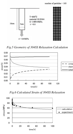
respectively. The plate is fixed at the top and the put primary load of 104MPa in the first time step. Then the end of the plate is fixed and relaxation is started. The primary elastic displacement is calculated and the total elastic and creep displacements are maintained constant in the all time steps. Yong’s modulus is 148919MPa. Figure 6 is the calculated elastic and creep strain of the plate. The creep strain increases and the elastic strain decreases in the condition of total strain is kept constant. Figure 7 is the calculated stress compared with the experimental result in the same condition (Asayama, T, 1999). The result is in good agreement with analytical one.

Fig.5 Geometry of 304SS Relaxation Calculation

0.00 0.01 0.02 0.03 0.04 0.05 0.06 0.07 0.08

0 20 40 60 80 100 120

time(h)

st

ra

in

(%

)

creep elastic total

Fig.6 Calculated Strain of 304SS Relaxation

0 20 40 60 80 100

0 20 40 60 80 100 time(h)

st

re

ss

(M

P

a)

calculation experiment

Fig.7 Calculated Stress of 304SS Relaxation

5. CONCLUSIONS

(10)

steady load is calculated. The result is compared with analytical and experimental results and is in good agreement with them. A tensile stainless steel plate with steady strain is analyzed. The stress relaxation with creep strain is compared with experimental results and is in good agreement with it.

REFERENCES

Nayroles, B., Touzot, G. and Villion, P.,''Generalizing the finite element method: diffuse approximation and diffuse elements'',Comput. Mech., 10(1992), 307-318

Belytschko, T., Lu, Y. Y. and Gu, L., ''Element-free malerkin methods'', Int. J. for Num. Meth. in Eng., 37(1994), 229-256

Yagawa, G., Yamada, T., Kawai, H., ''Free mesh method: a new finite element method'', Comput. Mech., 18(1996), 383-386

Koshizuka, S. and Oka, Y.,''Moving particle semi-implicit method for fragmentation of incompressible fluid'', Nucl. Sci. Eng., 123(1996), 421-434

Koshizuka, S., Nobe A., and Oka, Y., ``Numerical analysis of breaking waves using the moving particle semi-implicit method'', Int. J. Numer. Meth. Fluids, 26(1998), 751-769

Koshizuka, S., Ikeda, H, and Oka, Y., ``Numerical analysis of fragmentation mechanisms in vapor explosions'', Nucl. Eng. Des., 189(1999), 423-433

Chikazawa, Y., Koshizuka, S. and Oka, Y.,''Numerical analysis of sloshing with large deformation of elastic walls and free surfaces using MPS method''', Transactions of the Japan Society of Mechanical Engineers , 65-637, A(1999), 2954-2960, (in Japanese)

Chikazawa, Y., Koshizuka, S. and Oka, Y., "Numerical Analysis of Three-dimensional Sloshing in an Elastic Cylindrical Tank ysing Moving Particle Semi-implicit Method" Comput. Fluid Dynamics J. ,vol. 9, (2001), 376-383

Chikazawa, Y., Koshizuka, S. and Oka, Y., “A Particle Method for Elastic and Visco-plastic Structures and Fluid Structure Interactions”, Comp. Mech., vol. 27, (2001),97-106

Gingold, R. A. and Monaghan, J. J., `` Kernel estimates as basis for general particle methods in hydrodynamics'', J. Comput. Phys., 46(1982), 429-453

Blackburn, L.D., “Isochronous Stress-Strain Curves for Austenitic Stainless Steel”, The Generation of Isochronous Stress-Strain Curves (ed. A.O. Schaefer), ASME, pp15-48, 1972

Yoshitake, A., et al., “A statistical study of creep rupture and stress-strain behavior of structural materials under elevated temperature conditions”, Proceedings of Int. Conf. on Creep, 1986.