Modelling for Multidimensional
Environmental Analysis
Doc Thesis
byLei Song
Submitted in Partial Fulfillment of the Requirements of the
D.Comp. Program
Department of Computing and Information Technology UNITEC Institute of Technology
New Zealand March 2014
A variety of environmental problems increasingly attract academic research in order to protect ecosystems and minimise negative effects on human health. Advanced computational environmental analysis technologies have the potential to detect, monitor and perhaps effectively control these problems. However, computational environmental analysis is a complex and difficult problem to solve.
The problems associated with environmental analysis are the underlying data. These data are collected from sub-optimal positions in urban and rural areas. The limited number of monitoring stations in the network means that we are collecting enough samples over time, however, insufficient data samples are collected across the monitored area.
We determined the difficulty associated with computational analysis of environ-mental data via a critical review of existing approaches in the literature. Our review confirmed the biggest problem was associated with data collection, including noise introduced into the data stream, the big data problem in the form of an endless data stream, and missing data samples caused by ineffective equipment or poor place-ment of the monitoring equipplace-ment.
In this thesis, we document our research into computational environmental meth-ods for addressing land usage and air quality problems.
The detection of land use change is a process of identifying differences in the state of a phenomenon by observing time-lapsed landscape imagery. Motivated by a simple neural pattern recognition mechanism, we propose a novel “one-step-more” incremental learning change detection method. In this method, an agent discovers knowledge from the first image using pixel-level incremental learning. When we de-tect changes in the subsequent image, the discovered knowledge model is updated and ready for the next change detection iteration. This is what we have called the “one-step more” incremental learning method. Powered by incremental data mod-elling techniques, the system demonstrates the capability of continuously detecting time sequenced imagery. Additionally, the method is shown to be computationally inexpensive when initializing and updating the change detection model.
Land encroachment monitoring is essential to assist the economic growth, sus-tainable resource use and environmental protection of a city. We investigate land encroachment on public parks in the area of Auckland New Zealand, in which the proposed “one-step-more” method employed to analyse 26 Auckland parks. The obtained average region of interest (ROI) detection accuracy is 99.91% on five popu-lar park related objects i.e. fences, houses, parks, trees and roads. The effectiveness of the proposed method is demonstrated on four categories of encroachment:
methods for air quality analysis. The first investigation is indoor emission source detection and the second is outdoor air quality prediction. Emission source detec-tion indoors is important when locating the possible origin of polludetec-tion that could have a negative effect on the health of occupants. Outdoor air quality prediction is essential when attempting to minimise the negative effect on the health of citizens and the ecosystem.
Addressing indoor emission source detection, we propose a novel inter-pollutant correlation analysis technique. Unlike other documented solutions that analyze merely primary pollution, our method is further enhanced by calculating intra-pollutant correlation coefficients for characterizing and distinguishing emission events. Extensive experiments show that seven major indoor emission sources are identified by the proposed method, including (1) frying canola oil on electric hob, (2) frying olive oil on an electric hob, (3) frying olive oil on a gas hob, (4) spray of house-hold pesticide, (5) lighting a cigarette and allowing it to smoulder, (6) no activities, and (7) using an exhaust or ventilation system. Furthermore, our method improves the detection accuracy by a support vector machine, compared to the classification without data filtering, and with feature extraction of PCA and LDA.
Addressing outdoor air quality predication, we propose a novel spatial data-aided incremental support-vector regression (SaIncSVR). We overcome some of the problems associated with other prediction models. Existing models often demand data to be presented in a more convenient form than real data facilitates, for instance complete data, time-series complete, or a specified data capture process making them inadequate when used for environmental prediction. We conduct extensive experiments ofP M2.5 prediction over 13 monitoring stations in Auckland, New
Zealand. The experimental results indicate that our SaIncSVR performs improved P M2.5prediction. Our method shows the capability to overcome missing data
prob-lems, an improvement over many other documented techniques. We compare our method with a local incremental support-vector regression. Further forP M2.5
spa-tial prediction, we conduct experiments on outdoor air quality prediction using a data-driven Gaussian geometry model. This model shows promise on a limited number monitoring stations and warrants further investigations.
We promote incremental data modelling, given its benefits in processing large amounts of data with parallelization capability in many dimensions, as a construc-tive solution to spatio-temporal computational environmental analysis. This re-search documents systematic and comprehensive rere-search in the area of compu-tational environmental analysis. For this study we investigated a variety of en-vironmental problems, enen-vironmental data, change & emission source detection,
computational methods could be useful for other environmental detection and pre-diction problems, especially those using large, asynchronous and spatial-temporal data.
I would like to thank all people who have helped and inspired me during my doc-torate study.
This thesis was made possible by an Unitec Institute of Technology Scholarship. I am grateful to the Department of computing for the scholarship which enabled me to undertake a doctorate program at Unitec Institute of Technology.
I especially want to thank my supervisors, Assoc Prof. Paul Pang and Prof. Ab-dolhossein Sarrafzadeh, for their guidance during my research and study at Unitec Institute of Technology. Their perpetual energy and enthusiasm for research have motivated all their students, including me. In addition, Assoc Prof. Paul was always accessible and willing to help his students with their research. As a result, research life became smooth and rewarding for me. Many thanks also go in particular to Angelina Chai-Rodgers, for being supportive and helpful whatever the occasion.
My special words of thanks should also go to my industry supervisor, Dr. Ian Longley, for his constant motivation and support during the course of my thesis. I enjoyed the personal discussion with him to explore the idea for our collaborating projects. My sincere thanks to Dr. Gustavo Olivares for being with me as an domain expert. His scientific inputs, personal helps and friendly nature has always made me feel at ease with him. Without the encouragement as well as the access to their expertise and data this work would have not been possible.
All my lab buddies at the Doctorate Lab made it a convivial place to work. In particular, I would like to thank David McCurdy and Yiming Peng for their friend-ship and help during my thesis. All other folks, including Lei Zhu and Simon Dacey, had inspired me in research and life through our interactions during the long hours in the lab. Thanks.
My deepest gratitude goes to my family for their unflagging love and support throughout my life; this thesis is simply impossible without them. I am indebted to my father, Deguang Song, for his care and love. As a typical father in a Chinese family, he worked industriously to support the family and spared no effort to pro-vide the best possible environment for me to grow up and attend school. He had never complained in spite of all the hardships in his life. I cannot ask for more from my mother, Shuqing Hou, as she is simply perfect. I have no suitable word that can fully describe her everlasting love for me. I remember her constant support when I encountered difficulties and I remember, most of all, her delicious dishes
Last but not least, thanks be to God for my life through all tests in the past years. You have made my life more bountiful. May your name be exalted, honoured, and glorified.
AI Artificial intelligence ANN Artificial neural networks AR Autoregressive model
ARIMA Autoregressive integrated moving average model ARMA Autoregressive moving-average model
ART Adaptive resonance theory BME Bayesian maximum entropy EM Expectation-maximization FFT Fast Fourier transform GA Genetic algorithms
GTP Global temporal prediction HMM Hidden Markov models IOA Index of agreement KNN k-nearest neighbours LDA Linear discriminant analysis LTP Local temporal prediction MA Moving-average model
MBE Mean bias error
MLP Multi-layer perceptrons MRF Markov random field
PCA Principal component analysis RMSE Root mean square error RMSES Systematic RMSE
RMSEU Unsystematic RMSE
SaGTP Spatial data aided global prediction SaIncSVR Spatial data aided incremental SVR SVM Support vector machine
SVR Support vector regression
Abstract iv
Acknowledgements v
List of Abbreviations viii
1 Introduction 2
1.1 Background . . . 3
1.2 Computational Environmental Analysis and Challenges . . . 4
1.2.1 Pollution Detection . . . 5
1.2.2 Pollution Prediction . . . 7
1.3 Motivation of Incremental Data Modelling . . . 9
1.4 Environmental Problems Investigated . . . 9
1.4.1 Land Cover Change . . . 9
1.4.2 Indoor Air Quality Control . . . 9
1.4.3 Airborne Particulate Matter (P Mx) . . . 10
1.5 Approach . . . 10
1.5.1 Incremental Learning based Image Series Change Detection . 10 1.5.2 Pollutant Iteration Analysis and Online Emission Source De-tection . . . 11
1.5.3 Incremental Learning based Spatio-temporal Air Quality Pre-diction . . . 11
1.6 Contribution . . . 12
1.7 Thesis Organization . . . 12 ix
2 Environmental Data 14 2.1 Introduction . . . 14 2.2 Data Collection . . . 15 2.2.1 Environmental Surveying . . . 15 2.2.2 Monitoring Networks . . . 17 2.2.3 Remote Sensing . . . 17
2.3 Data Problems and Challenges on Data Analysis . . . 19
2.3.1 Noise . . . 19
2.3.2 Spatio-temporal Characteristics . . . 20
2.3.3 Endless Data Stream . . . 21
2.3.4 Missing Data . . . 22
2.4 Conclusion . . . 22
3 Environmental Change Detection 24 3.1 Introduction . . . 24
3.2 Computational Change Detection Methods . . . 25
3.2.1 Traditional Discriminant Methods . . . 26
3.2.2 State-of-the-art Methods . . . 28
3.2.3 Satellite Image Change Detection . . . 30
3.3 Performance Evaluation . . . 34 3.3.1 Accuracy . . . 34 3.3.2 Thresholding . . . 36 3.3.3 Sensitivity . . . 37 3.3.4 Continuity . . . 38 3.3.5 Discussion . . . 39
3.4 Applications to Environmental Problems . . . 39
3.4.1 Pollution Emissions . . . 40
3.4.2 Pollution Measurement . . . 40
3.4.3 Land Cover Change . . . 41
3.4.4 Ecological Upset . . . 42
3.5 Conclusion . . . 43
4 Environmental Prediction 45 4.1 Introduction . . . 45
4.2 Computational Environmental Prediction Methods . . . 46
4.2.1 Statistical Models . . . 46
4.2.2 Artificial Intelligence Models . . . 48
4.3 Performance Measurement . . . 55
4.3.1 Accuracy . . . 55 x
4.3.2 Dynamic Prediction . . . 56
4.3.3 Spatio-temporal Prediction . . . 57
4.4 Applications to Air Quality Control . . . 58
4.5 Conclusion . . . 59
5 Feature Extraction for Air Quality and Land Use Analysis 61 5.1 Introduction . . . 61
5.2 Air Quality Authentication . . . 63
5.2.1 Principal Component Analysis (PCA) . . . 63
5.2.2 Linear Discriminant Analysis (LDA) . . . 64
5.3 Land Use Image Understanding . . . 65
5.3.1 Gradient Feature . . . 65
5.3.2 Wavelet Feature . . . 66
5.4 Data Selection for Emission Source Categorization . . . 67
5.4.1 Term Frequency Sample Validation . . . 67
5.4.2 Pearson’s Correlation based Variable Selection . . . 68
5.5 Conclusion . . . 69
6 One-step-more Incremental Learning for Image Series Change Detection 70 6.1 Background . . . 70
6.2 Related Works and Motivations . . . 72
6.2.1 Existing Methods . . . 73
6.2.2 Image Series Change Detection . . . 73
6.2.3 Incremental Learning for Continuous Image Change Detection 74 6.3 Proposed Image Change Detection Method . . . 75
6.3.1 Image Feature Encoding . . . 76
6.3.2 Incremental Learning ofX1Objects . . . 77
6.3.3 One-step-more Incremental Learning on X2 for Change De-tection . . . 80
6.4 Experimental Results and Discussion . . . 83
6.4.1 Performance Evaluation Criteria and Robustness Test . . . 83
6.4.2 Region of Interest Detection . . . 84
6.4.3 Static Image Change Detection . . . 85
6.4.4 Image Series Change Detection . . . 85
6.5 Conclusions and Future Works . . . 87
7 Agent based Land Encroachment Detection 90 7.1 Introduction . . . 90
7.2 Related Work . . . 91
7.2.1 Applications of Land Encroachment Detection . . . 92 xi
7.2.2 Encroachment Detection Methods . . . 92
7.3 Agent-based Land Encroachment Detection . . . 95
7.3.1 Land Cover Feature Extraction . . . 96
7.3.2 Detection Model . . . 96
7.4 Experimental Results and Discussion . . . 97
7.4.1 Data . . . 97
7.4.2 Experimental Setup . . . 99
7.4.3 Region of Interest Detection . . . 100
7.4.4 Land Cover Detection Experimental Results . . . 101
7.5 Conclusions and Future Work . . . 104
8 Online Indoor Emission Sources Detection 105 8.1 Introduction . . . 105
8.2 Related works . . . 106
8.3 Methodology . . . 108
8.3.1 Time Series Analysis . . . 108
8.3.2 Data Filtering . . . 109
8.3.3 Incremental SVM Classification . . . 110
8.4 Experimental Results and Discussion . . . 111
8.4.1 Data Set Description . . . 111
8.4.2 dataQA . . . 112
8.4.3 Extracted Knowledge from the Proposed Method . . . 113
8.4.4 Accuracy . . . 113
8.4.5 Sensitivity and Robustness . . . 116
8.5 Conclusions . . . 117
9 Online Spatio-temporalP M2.5Prediction 119 9.1 Introduction . . . 119
9.2 Related Works . . . 120
9.2.1 Ratio Prediction . . . 120
9.2.2 Tracer Model . . . 121
9.2.3 Methods for Spatio-temporalP M2.5Prediction . . . 123
9.3 Methods . . . 123
9.3.1 SaIncSVR: Spatial Data AidedP M2.5Prediction . . . 124
9.3.2 A Solution toP M2.5Spatial Prediction . . . 127
9.4 Experimental Results and Discussion . . . 129
9.4.1 Data . . . 129
9.4.2 Experimental Setup . . . 130
9.4.3 Performance Evaluation . . . 130 xii
9.4.4 Applying Spatial Data in Temporal Prediction . . . 132
9.4.5 Spatio-temporalP M2.5Prediction . . . 139
9.4.6 SpatialP M2.5Prediction . . . 139
9.5 Conclusion . . . 141
10 Conclusion and Future Works 144 10.1 Conclusion . . . 144
10.2 Future Works . . . 146
References 149
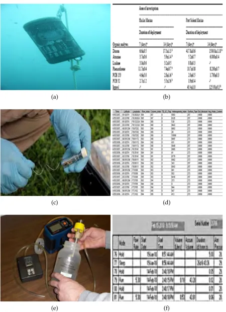
2.1 An example of grab samples: 2.1a filling a clean bottle with river wa-ter, 2.1b determining the level of chemical parameters in wawa-ter, and 2.1c recording the chemical parameters. . . 16 2.2 An example of passive sampling: 2.2a chemcatcher for water quality
data collection, 2.2b data returned from chemcatcher water sampling, 2.2c chemcatcher for soil quality data collection, 2.2d data returned from chemcatcher soil sampling, 2.2e air sampling pump for air qual-ity data collection, and 2.2f air qualqual-ity data returned from passive sampling. . . 18 2.3 An example of continuous data collection: 2.3a real-time water
qual-ity monitoring, 2.3b raw data of real-time water qualqual-ity monitoring, 2.3c real-timeP Mxmonitoring, and 2.3d raw data of real-timeP Mx
monitoring. . . 19 2.4 An example of remote sensing data collection: 2.4a real-time land
cover in New Zealand (visible wavelengths), 2.4b the temperature data of New Zealand from satellite (invisible wavelengths). . . 20 2.5 An example of spatio-temporal Data. . . 21 4.1 A neural network is an interconnected group of nodes. . . 51 4.2 The inputxis transformed into a 3-dimensional vectorh, which is
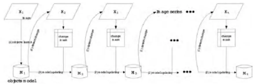
then transformed into a 2-dimensional vectorg, which is finally trans-formed intof. . . 51 6.1 Illustration of one-step-more incremental learning for image series
change detection. . . 72 xv
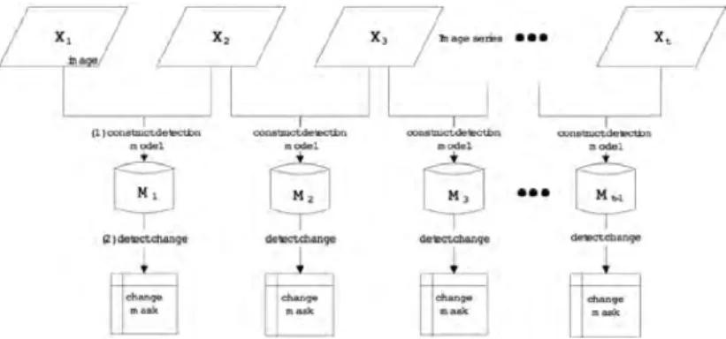
6.2 Graphical representation of existing image change detection methods for image series change detection. . . 74 6.3 Graphical representation of incremental learning based image series
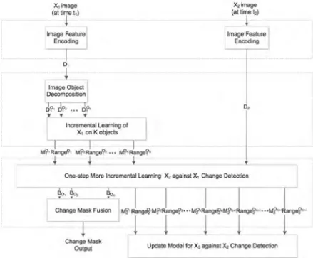
change detection. . . 75 6.4 The diagram of proposed agent-based incremental learning image
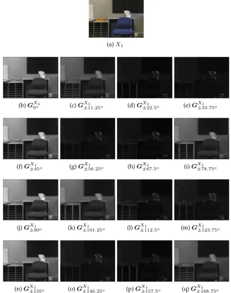
change detection system. . . 76 6.5 An original imageX1and the corresponding magnitudes of the
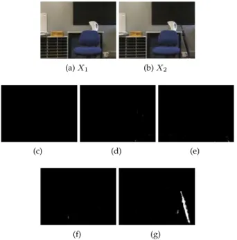
complex-valued directional subbands. . . 78 6.6 Change detection conducted on different objects (c)BO1, (d)BO2, (e)
BO3, (f)BO4, (g)BO5. . . 81 6.7 The change detection mask, BCM, resulted by merging all 5 binary
masks according to (6.13). . . 82 6.8 5 scenarios in a computer lab to cover case study of light condition,
background. . . 84 6.9 Change detection results using different sets of images: (a) Input
im-agesX1, (b) Input imagesX2, and (c) final change detection masks BCM. . . . 86 6.10 Change detection results using a sets of images: (a) is the source
im-ageX1and (b) to (e) are target imagesX2toX5. (f) to (i) areBCMs
for each step of change detection. . . 87 6.11 Computational costs comparison, proposed method vs. unsupervised
learning change detection. . . 88 6.12 Memory usage comparison, proposed method vs. simple
differenc-ing method. . . 89 7.1 The process of applying one-step-more incremental learning method
for land encroachment detection. . . 95 7.2 5 scenarios to cover case study of changes on fences, house, trees,
roads and park areas. . . 100 7.3 The scenario of land encroachment detection on Wyllie Park. . . 102 7.4 The scenario of land encroachment detection on Teviot Reserve. . . . 102 7.5 The scenario of land encroachment detection on Auburn Reserve. . . 103 7.6 The scenario of land encroachment detection on Diana Reserve. . . . 104 8.1 The procedure of subsequences extraction, whereXis time series and
cis slide window. . . 109 8.2 The experiment room. . . 112
8.3 (a) Levels of organic contaminants obtained from PACMAN for event “Frying canola oil, electric hob”; (b) levels of organic contaminants obtained from PACMAN for event “Smoking”; (c) the native organi-zation of organic contaminants for the two events with session “Vent-ing” and “Normal” distributes on 3D space; (d) deterministic compo-nents obtained after data filtering for event “Frying canola oil, elec-tric hob”; (e) deterministic components obtained after data filtering “Smoking”; (f) the filtered data for the two events with session “Vent-ing” and “Normal” distributes on 3D space. . . 114 8.4 The comparison of truth positive accuracy for 7 emission events
clas-sification. . . 116 8.5 The trend of the performance of target feature extraction methods. . 117 9.1 Spatial prediction assumption. . . 128 9.2 Three dailyP M2.5 prediction methods (a) local temporal prediction
(LTP), (b) global temporal prediction (GTP), and (c) spatial data aided global prediction (SaGTP). . . 133 9.3 The difference between SaGTP and other two methods in prediction
error for the period from2ndJanuary, 2012 to1st February, 2012 on
station Gavin Street. . . 134 9.4 The difference between SaGTP and other two methods in prediction
error for the period from2nd January, 2011 to31st January, 2012 on
station Wairau Road. . . 135 9.5 The difference between SaGTP and other two methods in prediction
error for the period from18thMarch, 2011 to17thApril, 2011 on
sta-tion Edinburgh Street. . . 136 9.6 The difference between SaGTP and other two methods in prediction
error for the period from5thApril, 2011 to6thMay, 2011 on station
Shakespear Park. . . 137 9.7 P M2.5spatial prediction model illustration in (a) 2D and (b) 3D spaces.142
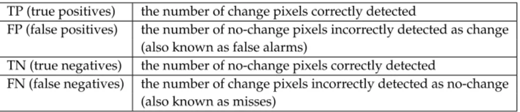
3.1 The Quantity Evaluations of Change Detection Accuracy . . . 35 3.2 Evaluation of Change Detection Methods According to The Proposed
Method Evaluation Criteria . . . 39 4.1 SVM Kernels . . . 54 5.1 Kernels of Well-known Image Edge Operators . . . 66 6.1 Change Detection Performance Results of Incremental Learning
Im-age Change Detection on Tasks with 5 Scenarios . . . 84 7.1 ROI Detection of Agent-based Image Change Detection on Tasks with
5 Scenarios . . . 101 8.1 A Summarization of The Notation Used in This Chapter . . . 108 8.2 Summary of Measured Parameters and Sensors in The PACMAN Units111 8.3 A Comparison of Algorithms Using Classification Accuracy in
Per-centage as a Prototype . . . 115 8.4 Performance of Target Feature Extraction Method in Different Size of
Sliding Windows . . . 117 9.1 Description ofP Mx datasets from 13 Monitoring Stations in
Auck-land, New Zealand . . . 131 9.2 Results of LTP, GTP and SaGTP DailyP M2.5 Prediction for Station
Gavin Street, Wairau Road, Edinbourgh Street and Shakespear Park. The Period of Prediction is from January, 2011 to December, 2012 . . 138
9.3 SaIncSVR Versus IncSVR for Spatio-temporalP M2.5prediction on 13
monitoring stations in Auckland New Zealand. . . 140 9.4 Spatial Prediction on 6 Monitoring Stations in Auckland New Zealand
Chapter 1
Introduction
Environmental issues have gained an increasing prominence on a global scale in re-cent times. As stated in (Fransson & G¨arling, 1999), a serious threat to human beings and their environment is the continuous and accelerating overuse and destruction of natural resources. People have made great efforts to protect the environment and preserve their way of life. Unfortunately, many of the environmental problems that have attracted the most public attention, such as global warming, deforestation, and so on are becoming even worse than thought.
Up to now, a numbers of efforts have been made in addressing the environmen-tal issues, chief among them the problems of climate change, global warning, Ozone depletion, and so on. The digitization of our world has been a forward processing now; still, it is surprising to step back and look at the physical change of the en-vironment. People now monitor emission sources in road transport, air quality in urban areas, ground water quality, sea level, satellites images on land usage, and so on by digital sensors. As a result, there is a huge amount of data, returned from monitoring stations, that satisfies compliance obligations and can be mined to pro-vide insight and information about the environment. The database includes satel-lite photos, cartographic information, and the results of all aspects of environmental studies, which provides a efficient digital library to support environment treatment. Computational environmental analysis conducts knowledge discovery from data for decision making support towards environmental treatment, which covers specif-ically pollution detection (monitoring), examination, and prediction. Among them, pollution detection identifies where and what pollution happens to make an intel-ligent measure of the environmental changes by collecting real-time data on emis-sions, weather conditions or land covers; pollution examination evaluates the level of pollution and effects of pollutants to investigate the relationship between mea-sures of pollution, such as air quality or proximity and presence of industrial fa-cilities; and pollution prediction estimates the future trend of pollution to identify the best management practices that control pollutant losses. In general, computa-tional environmental analysis presents important information for government envi-ronmental agency as well as envienvi-ronmentalists to prevent pollution.
doctorate thesis research lies in:
• Environmental change. Environmental analysis is a systematic process ini-tiated by detecting changes in terms of classification and location of those changes. Given an environmental change has been detected this can trigger the possibility of performing statistical analysis to understand potential causes of that change, thereby yielding a classification (reason and type). The location of pollution (especially in motion) poses problems for environmental change detection and perhaps overlooked by many researchers, owing to the actual and perceived complications of dynamic environmental change detection.
• Air quality. Environmental issues are induced by pollutants in air, soil and water resources. The air is a complex dynamic natural gaseous system that provides essential gas to support life on planet Earth. Pollutants, that are de-livered to the surrounding air, have hazard consequences to human and na-ture. This has been a significant risk factor for multiple health conditions. The health effects results from air pollution include difficulty in breathing, wheez-ing, coughwheez-ing, asthma and aggravation of existing respiratory and cardiac con-ditions. Air pollution, cause enormous external costs; as a consequence the air pollution prevention takes a significant role.
1.1
Background
Environmental problems are some of the most serious problems to affect peoples’ lives. Pollution causes unpredictable diseases and disasters; it even brings deadly threats to people. The main forms of pollution are air, water and soil pollution. Pollution is defined as the process of making air, water, soil dangerously dirty and not suitable for people to use, or the state of being dangerously dirty.
1. Air pollution. Air pollutants (WHO, 2005) include many different types, such as sulfur oxides, carbon monoxide, pesticides and fluorides. Also, air pollu-tion has some harmful effects on humans, animals, plants, or other materials in the environment. For example, carbon monoxide could impair the blood’s ability to transport oxygen.
2. Water pollution. Water pollutants (West, 2005) include a broad variety of ma-terials, like synthetic organic compounds, human and animal wastes, radioac-tive materials, heat, acids, sediments, and disease-causing microorganisms. Similar as air pollution, water pollution could also cause damaging issues on humans, animals and environment. For example, the element mercury is used
for producing light switches, air conditioners, fluorescent lights, etc. When such things are made, small amount of mercury metal is likely to escape into the environment and, eventually, into lakes and rivers. As known, mercury is highly toxic to living creatures.
3. Soil pollution/Land pollution. Soil pollution (Soil Pollution, 2011) contains the pollutant materials of soils, mostly chemicals. Soil pollution can lead to water pollution if toxic chemicals leach into groundwater, lakes, or oceans. It also gives rise to air pollution, because soil may release volatile compounds into the atmosphere. It is obviously harmful to plants and has destructive effect on living animals.
In order to cope with pollution problems, people have spent lots of money and efforts on establishing an effective strategy. Moving manufacturers to downwind position, recycling waste, educating people the importance of environmental pro-tection to analyzing environmental problems, investigating pollutants, people have done many works on pollution prevention. Apparently, all the above efforts are not sufficient, as we know global warming, ozone hole, melting glaciers and “big smoke” etc are getting worse with the time going on.
1.2
Computational Environmental Analysis and
Chal-lenges
Computational environmental analysis uses techniques, derived from fields like computer science and applied mathematics, to simulate and analyze computational models for environmental problems. Statistical analysis and machine learning meth-ods have been widely applied to environmental analysis on account of their advan-tages on fast and effective calculation (Ratle, Kanevski, Terrettaz-Zufferey, Esseiva, & Ribaux, 2007; Rebenitsch, Owen, Ferrydiansyah, Bohil, & Biocca, 2010; Schwen-der, Zucknick, Ickstadt, & Bolt, 2004). In addition, remote sensor techniques, which are also widely used, allow people to observe most environmental problems. There-fore, computational environmental analysis is one of the solutions to environmental problems.
Computational environmental analysis includes pollution detection (monitor-ing), pollution examination and pollution prediction (Raes, Foerstner, & Bork, 2007; Kreinovich et al., 2007; Rangel, Diniz-Filho, & Bini, 2006). Pollution detection identi-fies where and what pollution happens. Pollution examination evaluates the level of pollution and effects of pollutants. Pollution prediction estimates the future trend
of pollution. Computational environmental analysis presents important informa-tion for environmentalists to prevent polluinforma-tion.
1.2.1
Pollution Detection
Pollution Detection is used to identify the location and types of pollution in the environment. It can be described as:
1. changes in pollutants, increases and decreases in quantity, severity, etc,
2. and introduction of new types of pollutants.
Change detection is also the fundamental tool for pollution analysis, which provides the useful information to pollution examination and pollution prediction.
Environmental change detection has four requirements as detection accuracy, automatic detection, detection sensitivity, and detection continuity. Detection ac-curacy reports exactly all differences amongst a series of variables for each data collection. Automatic detection dynamically adjusts thresholds of change detection methods. To achieve early warning, the sensitivity of change detection is impor-tant for environmental analysis in that an environmental problem cannot happen within one day, there is a procedure of environmental change before the problem becomes serious and widely recognizable (Fries, Ziegler, Kurian, Jacoris, & Pollak, 2005). Environmental changes may be rapid and significant or slow and inconspic-uous. Such changes actually continue over time, possibly without end. Thus, con-tinuous change detection with high speed is also important.
Applications
In fact, environmental change detection works as cleaning equipments and air / wa-ter indicators for monitoring environmental system (Matsuzawa et al., 1984; Francke, Miessner, & Rudolph, 2000; Carlton & Smith, 2000). Since the advancement of re-mote sensing technology and improvement of satellite images resolution, it then has been applied on area surveillance / land cover changes detection (Vu, Matsuoka, & Yamazaki, 2004; Haverkamp & Poulsen, 2003; Phua, Tsuyuki, Furuya, & Lee, 2008). Furthermore, for the purpose of ecological restoration, environmental change detec-tion for image data also plays a very important role, because environmental change detection can accurately presents what happened in the target area (Ardli & Wolff, 2009; Fortin et al., 2000).
Current issues
For performance evaluation, typical environmental change detection concerns change detection accuracy and convenient threshold determination. However, the study of sensitivity and continuity of change detection has attracted limited attention so far. Early pollution detection and long term monitoring are the current issues for envi-ronmental change detection.
• Detection sensitivity. Sensitivity for change detection refers to the capability for detecting minute changes that are imperceptible and easily neglectable. Note that sensitivity here is different from accuracy, and it can be obtained by just setting narrow thresholds and detecting more changes. It detects where/what changes when it first happens and reports not only percentages, but also the probability of pollution.
Existing change detection methods consider merely accuracy of the detection. Actually, the high sensitivity is not equivalent to the high accuracy. The sen-sitivity is limited because existing methods report only one specific variable based on interaction among all variables (Klanova, Kohoutek, Hamplova, Ur-banova, & Holoubek, 2006; Martinez, Phillips, & Whitesides, 2008; Fischer, Dryer, & Curran, 2000; Loomis, Castillejos, Gold, McDonnell, & Borja-Aburto, 1999; Dagan, 2000).
In addition, existing change detection methods enhance the sensitivity via nar-rowing the thresholds. However, narrowed thresholds not only filter out slight changes but also amplify the effect of noises. This leads to more false alerts.
• Detection continuity. Continuous change detection is to track environmental changes from an uninterrupted environmental variations. A typical exam-ple is biological invasions. Biological invasions are defined as breach biogeo-graphic barriers and extend their range. Invasions of nonnative plants, ani-mals, or microbes cause major environmental damage. Though human has attempted to manage biological invasions for long time, but invasions con-tinuously occur among rivers, lakes and canals, even if they are very clean (Vitousek, D’Antonio, Loope, & Westbrooks, 1996). Monitoring environmen-tal changes like biological invasions demands for long term environmenenvironmen-tal change detection. In general, the difficulties of continuous environmental change detection are given below:
1. environmental data comes in real time;
2. environmental change involves huge size of data stream or matrix; 3. environmental data comes with unknown pollutants;
4. environmental changes are required to be detected instantly without re-training detection model.
It is worth noting that existing change detection methods perform very lim-ited on continuous environmental change detection, because they are not ca-pable to process for large amount of data stream such us huge amount of en-vironmental data. Two limitations of the existing change detection methods to achieve continuity are, 1) the change detection can only be conducted by comparing samples one by one, and 2) the thresholds can only be determined and fixed according to previous experience. Because both sampling and re-setting thresholds cost much time, a great number of changes may be missed during the process.
1.2.2
Pollution Prediction
Pollution prediction simulates the progress and estimates the future trend of pol-lution based on the information retrieved by polpol-lution change detection system. It helps stakeholders construct strategies to deal with pollution problems. Analog to most prediction problems, pollution prediction suffers when data lose and special events happen.
Applications
Pollution prediction is important for people to decide strategies on special environ-mental problems after disasters. Bombay city used to predict concentrations of car-bon monoxide (CO) with models like GM, CALINE-3 and HIWAY-2, which reports air pollution for the government to decide traffic system (Luhar & Patil, 1989). A case in Slovenia is to predictSO2from coal fired thermal power plants for advising
the government to develop new energy and control the quantity of provided power (Boznar, 1997). Global ocean pollution caused by oil spill is one of the most serious problems to people and marines. Hackett, Comerma, Daniel, and Ichikawa (2009) shows the directing applications and strategies for pollution prevention based on oil spill fate forecasting systems.
Current issues
• Data Missing. Data missing problem is a serious issue for all prediction mod-els. The input of prediction models is the most important (Barlow et al., 6 September 2006; Iimura et al., 2009), whereas environmental data analysis has confronted with serious data missing situations, because new pollutants are
continuously presented (Guo, Jia, Pan, Liu, & Wichmann, 2009). Until now, en-vironmentalists still cannot predict Fukushima nuclear leakage 2011, because a great amount of unknown pollutants came up after this disaster and it was the first time that nuclear pollutants exhausted to ocean.
• Special events. Special events sometimes may lead prediction models to pro-duce incorrect forecasts to people. Special events bring new pollutants and new pollution types to environmental analysis without any experience. In other prediction applications such as finance (Pang, Song, & Kasabov, 2011) and medical science (Kanehisa et al., 2008), similar patterns can be extracted from historical data. However, environmental analysis usually confront with pollution types when pollution generated from new technologies. Thus, dif-ferent from other applications, it is very difficult to perform pollution predic-tion successfully after special events.
• Spatial consideration. Existing air quality prediction projects focus on apply-ing spatial characteristics to support time series forecastapply-ing. Prediction mod-els such as Bayesian Maximum Entropy (BME) method and Hidden Markov Models (HMM) has been applied on spatio-temporal air quality prediction. BME models are often used with ratio prediction such as ratio ofP M2.5/P M10,
which store the ratios for the different locations (Chang & Lee, 2008). HMM applies probabilities on air quality prediction, the regression function can be simulated by Markov chains, which provides more accurate forecasting (Dong et al., 2009). However, HHM models calculate the probabilities with geograph-ical characteristics, it is a way to consider spatial information but not spatial prediction.
• Prediction continuity. Considering the latest change in the air is another hard topic for air quality prediction. Due to changes in the air occurring all the time, a self-updated learning model is required. However, BME models provide a storage for time series prediction models in different location. If a change happen, BME models must be retrained for each location (Chang & Lee, 2008; Christakos & Serre, 2000). HHM models have the same problem as the BME models. If a change happens, all the input probabilities must be re-calculated, which incurs an expensive calculating cost and is time consuming (Schmidler, Liu, & Brutlag, 2000; Dong et al., 2009) .
1.3
Motivation of Incremental Data Modelling
Environmental problems comprise information from both location and time. Inte-grating data from different spatial and temporal scales is an important component of computational environmental study. Environmental problems, however, which are commonly temporally rich in data, but haven’t motivated extensive spatio-temporal environmental studies in literature. This results existing solutions to computational environmental analysis focus on trace of local problems rather than a spatio-temporal analysis. In this research, we consider incremental data modelling for spatio-temporal environmental analysis, owing to the following advantages of incremental learning,
1. capability of keeping all knowledge in memory while learning with protection from forgetting,
2. capability of mining a large amount of data with parallelization on spatial and temporal dimensions.
1.4
Environmental Problems Investigated
Environmental problems are complex, ever changing, and are the subject of many research papers in various disciplines. In this thesis, we address specifically three major environmental problems which are land cover change, indoor air quality and airborne particulate matter.
1.4.1
Land Cover Change
Land cover change is categorized as proximate (direct, or local) and underlying (in-direct or root). The proximate change is caused (in-directly by humans operating at the local level (e.g., individual farms, households, or communities), while the un-derlying change is caused by broader context and fundamental forces underpinning these local actions originating from regional (e.g., districts, provinces, or country). Land cover change effects biotic cover, water quality, hydrological, water flows and biological impacts. Deforestation and encroaching shrubland are two typical phe-nomenons of land cover change, which may eventually cause flooding and shortage of agricultural land.
1.4.2
Indoor Air Quality Control
People spend about 80% of time indoors, so it is important that we gain a better understanding of the pollutants to which people are exposed indoors. Common
in-door sources of airborne particles include combustion sources (e.g., primarily heat-ing and cookheat-ing) and tobacco smokheat-ing. Other sources include combustion (e.g., candles, incense, etc), hygiene products (e.g. solvents, pesticides) and activities (e.g. dusting). Identifying the contribution of each source, and exposure to it, is central to the effort to understand health effects and manage risks. The magnitude, fre-quency and prevalence of these sources are strongly related to individual lifestyles and behaviours.
1.4.3
Airborne Particulate Matter (P M
x)
Air pollutants emitted by pollution sources are usually categorized to suspended particulate matter (P M) (e.g., dusts, fumes, mists, and smokes); gaseous pollutants (e.g., gases and vapors); and odors. P M, one of the major pollutants, is tiny solid and/or liquid particles suspended in the air. These particles can be classified accord-ing to total suspended particles: the respirable suspended particleP M10 (median
aerodynamic diameter less than 10.0 microns), and the fine particles P M2.5
(me-dian aerodynamic diameters of less than 2.5 microns). P Mxleads to increased use
of medication. The health effects made byP Mxinclude coughing, wheezing,
short-ness of breath, aggravated asthma, lung damage (including decreased lung function and lifelong respiratory disease), premature death in individuals with existing heart or lung diseases. Since the size ofP M2.5is very tiny, it travels deeper into the lungs.
ThereforeP M2.5can have worse health effects than theP M10.
1.5
Approach
Existing solutions for spatio-temporal environmental analysis process their data from a huge storage system through a specific batch learning model. In the ap-proach, the learning model not only considers information from both spatial and temporal domains, but also the model updates itself when the latest change occurs without expensive computational costs and high memory usage.
1.5.1
Incremental Learning based Image Series Change Detection
Environmental data such as flooding, deforestation and land use data are moni-tored by satellite images, they are not a pair of image and only contain a single object. However, existing image change detection methods focus on seeking dif-ferences between a pair of images (Im, Jensen, & Tullis, 2008a; Ma, Zheng, Yuan, & Zhang, 2010; Verbesselt, Hyndman, Zeileis, & Culvenor, 2010). For image series change detection, existing methods generally rely on tracking a foreground objectto detect the changes across different images (Tian, Feris, Liu, Hampapur, & Sun, 2011; Borges & Izquierdo, 2010). No existing image series change detection solution offers a general solution for continue and multiple objects detection.
This thesis proposes that one-step more incremental learning for image series change detection, which allows an agent to upgrade its knowledge on the target image by performing incremental learning on top of its current knowledge. By rec-ognizing major objects, the proposed method can learn knowledge from the current image for change detection. As this thesis shows, the one-step more incremental learning model can be self-updated when new knowledge comes, allowing image change detection explicitly to make a trade-off between performance and consis-tency in the evaluation of accuracy and continuity.
1.5.2
Pollutant Iteration Analysis and Online Emission Source
De-tection
There are many reasons an emission source detection system should offer an effec-tive knowledge discovery component by which applications can extract the most important features from their data. A detection system supported by a feature extraction system already has an established developer base, making it effective for emission source detection. So far, many pattern recognition models have been used to detect emission sources. These extraction methods are used to magnify the main orthogonal contributions which explain most of the pollutants for an emission source. Therefore it is hard to consider the interaction between pollutants.
The knowledge extraction method in this thesis, on the other hand, instead mag-nifies the main pollution contributions: the relationships among pollutants. This is a correlation coefficient based approach to support emission sources detection. Fur-thermore, this approach considers the relationship among pollutants in comparison with other existing feature extraction methods. Therefore the detection results sup-ported by the proposed method are better than the detection results supsup-ported by other feature extraction methods.
1.5.3
Incremental Learning based Spatio-temporal Air Quality
Pre-diction
Ideally environmental events prediction model should be able to achieve three cri-teria: accuracy, spatio-temporal consideration, and real time prediction. Existing prediction models focus on applying geographical characteristics on time series pre-diction models to improve the forecasting accuracy rather then considering spatial
information. In addition, existing models are not able to carry on the latest change in the air with updating itself only.
This thesis proposes a spatial prediction forP M2.5forecasting and incremental
learning models to catch the latest changes in the air. The spatial prediction ap-proach supposes that the concentration ofP M2.5gradually decreases from the city
center outwards to rural area. We can then provide a set of concentric rings in order to predictP M2.5in a range for related (i.e. locations based on the same ring)
loca-tions. In addition, this research applies incremental learning SVR to add new data into the support vector machine by updating SVM model only.
1.6
Contribution
The main contributions of this thesis are as follows:
1. proposes a novel incremental learning based image change detection method capable of detecting sequences of changes over image series,
2. calculate in-between pollutants correlation coefficients for characterizing and distinguishing emission events,
3. applies spatial prediction to analyse the relationship between the strength of P M2.5concentrations and distance to city center,
4. and utilizes incremental learning SVM regression to consider the latest change in the air, which means re-training learning models without high computa-tional cost when the latest data comes.
1.7
Thesis Organization
The rest of this thesis is organized as follows. Chapter 2 explores the data and data collection on different environmental problems and highlights the challenges that we address for computational environmental analysis. Chapter 3 evaluates envi-ronmental change detection methods with a focus on the envienvi-ronmental problems addressed by the thesis. Chapter 4 gives a brief introduction to environmental pre-diction models with a focus on air pollution prepre-diction. Chapter 5 discusses fea-ture extraction researches which have been conducted on land use problems and air pollution. Chapter 6 proposes a one-step more incremental learning approach to image series change detection, and Chapter 7 applies the approach to land en-croachment detection of Auckland parks. Addressing air quality problem, Chap-ter 8 proposes a correlation based feature extraction method to support emission
source detection system. Chapter 9 proposes a spatial prediction forP M2.5
concen-trations in Auckland region, and measures the performance of incremental learning for spatio-temporalP M2.5 concentration forecasting. Finally, Chapter 10 contains
Chapter 2
Environmental Data
Environmental data reflects the variation of environmental conditions. We analyse the data for the purpose of understanding environmental behaviors in statistic. Typ-ically, the data is collected by monitoring networks and remote sensors. This chapter explores the data and data collection on different environmental problems and high-lights the challenges that we address for computational environmental analysis.
2.1
Introduction
Environmental problems are harmful aspects of human living conditions and bio-physical environment. Environmental data describes environmental pressures, the state of the environment, and the impacts on ecosystems. Environmental data col-lection covers all environmental problems from indoor air pollution to climate mi-gration and from soil nutrition to farmland sandy desertification.
The environmental data and statistics are relevant to city planning. In a city, a monitoring network that consists of a number of distributed stations is operating for monitoring the drink water quality, air pollution pressures and land usage. Such continuous data collection serves a vital role on city environmental management by revealing long-term trends that can lead to new knowledge and understanding, and planning environmental policy.
In practice, environmental data collection is highly influenced by many natural phenomena such as lighting and windy, equipment failure, insufficient sampling or measurement errors. This pose great challenges on computational environmental analysis, to handle noisy, spatio-temporal, full of missing samples, and continuously streaming data.
This chapter is organized as follows: In section 2.2, we present the brief con-cepts of environmental data collection. In Section 2.3, we discuss the status of en-vironmental data and challenges to computational analysis. Finally, a conclusion is provided in Section 2.4.
2.2
Data Collection
Environmental data is collected for the preparation of environmental impact anal-ysis, as well as in many circumstances in which human activities carry a risk of harmful effects on the natural environment. In all cases the collected data will be reviewed, analysed statistically and published to the public. In a city, the environ-mental pressures are mostly from energy, population pressures, transportation, and waste. The monitoring items often include air quality, amenity, biodiversity, land, natural hazards and water. The data collection methods generally can be categorised as environmental surveying, auto continuous monitoring, and remote sensing.
2.2.1
Environmental Surveying
Environmental surveying uses surveying techniques to understand the potential impact of environmental factors on humans life. The surveying collects environ-mental data casually and perhaps irregularly, this includes grab sampling and pas-sive sampling. Environmental surveying is a popular approach used in environ-mental monitoring, as it is simple and accurate. However, the equipment used for chemical parameter identification can be highly expensive.
To analyse a homogeneous material, for example water, the often used collec-tion method is “grab samples”. A very common example of grab samples is to fill a clean bottle with river water. This method provides a good snap-shot view of the quality of the sampled environment at the location of sampling and at the time of sampling. After collection, the sampled water is analysed under chemical environ-ment to produce the level of chemical parameters that have the potential to affect any ecosystem. The list of chemical parameters can be expanded or reduced based on developing knowledge and the outcome of the initial surveys (Felipe-Sotelo, An-drade, Carlosena, & Tauler, 2007). The grab samples method is useful in explaining the inhibition mechanism but they are often expensive and time-consuming (Gece & Bilgic¸, 2009). In addition, the data collected cannot be extrapolated to other times or to other parts of the river, lake or ground-water without additional monitoring (Nollet & De Gelder, 2000). Figure 2.1 shows an example of grab samples for water data collection.
“Passive sampling”, another environmental surveying, reduces the cost and the need of infrastructure on the sampling location. This method allows for a better cover and more data being collected. Chemcatcher and an air sampling pump are the examples of a passive sampling devices. Figure 2.2 shows the chemcatcher for water/soil quality data collection and an air sampling pump for air quality data collection. Although passive sampling provides clearly the particle phase of the
(a)
(b)
(c)
Figure 2.1: An example of grab samples: 2.1a filling a clean bottle with river water, 2.1b determining the level of chemical parameters in water, and 2.1c recording the chemical parameters.
atmosphere, water or soil, the data collected cannot be extrapolated to other times or to other place.
2.2.2
Monitoring Networks
As the requirement from the public, many environmental status such as drink wa-ter quality and air quality must be reported real-time. Therefore environmental data collection is required to be a continuous work, which involves having an automated collection close to the environment being observed so that data can be monitored in real time. There are a large number of specialized sampling equipments avail-able that can be programmed to take samples at fixed or variavail-able time intervals or in response to an external trigger. For example a sampler can be programmed to start taking samples of air chemical parameters (P Mx,N Ox) of a monitoring
sta-tion at 1-minute intervals. Such systems are often established to protect important water supplies and air quality monitoring for early warning of potential problems. These systems routinely provide data of chemical parameters such as pH, dissolved oxygen, conductivity, turbidity and colour in the water andSO2,N O2,CO,O3and
P Mx in the air to examine a wide range of potential organic pollutants. Figure
2.3 gives an example of continuous environmental data collection for water and air quality from the national institute of water and atmospheric research (NIWA), New Zealand.
2.2.3
Remote Sensing
The urban sprawl and forest coverage decreasing are national or global problems and happen in a large area. Problems such as climate change, global warming and rainfall also varies over the time and in large areas. Remote sensing is an important technique for monitoring such environmental problems.
For remote sensing, aircraft or satellites are used to monitor the environment by multi-wavelengths sensors. The visible wavelengths (RGB), known as true color images, are often used for land use problems such as area surveillance, ice fields, deforestation, flooding and so on. The invisible wavelength is represented by value of electromagnetic energy and mapped into a false color satellite image. These false color images are often used for monitoring clouds, Earth’s vegetation, atmospheric trace gas content, sea state, ocean color. Figure 2.4 shows two examples of remote sensing images for land cover and temperature monitoring in New Zealand.
(a) (b)
(c) (d)
(e) (f)
Figure 2.2: An example of passive sampling: 2.2a chemcatcher for water quality data collection, 2.2b data returned from chemcatcher water sampling, 2.2c chemcatcher for soil quality data collection, 2.2d data returned from chemcatcher soil sampling, 2.2e air sampling pump for air quality data collection, and 2.2f air quality data re-turned from passive sampling.
(a) (b)
(c) (d)
Figure 2.3: An example of continuous data collection: 2.3a real-time water quality monitoring, 2.3b raw data of real-time water quality monitoring, 2.3c real-timeP Mx
monitoring, and 2.3d raw data of real-timeP Mxmonitoring.
2.3
Data Problems and Challenges on Data Analysis
Environmental data have problems such as noise, spatio-temporal, endless data stream, and missing data. This problems makes a number of challenges in com-putational environmental analysis. This section explores the challenges from those problems.
2.3.1
Noise
Noise is often involved in environmental data. Natural ventilation, weather condi-tion and equipment failure is the main causes of noise in air quality data colleccondi-tion (Scrimger, 1985). Raining, hailing and snowing often affects the quality of under-water data (Scrimger, 1985). Lighting, cloudy and weakness of spectral resolution
(a) (b)
Figure 2.4: An example of remote sensing data collection: 2.4a real-time land cover in New Zealand (visible wavelengths), 2.4b the temperature data of New Zealand from satellite (invisible wavelengths).
makes a numbers of speckle noise on satellite images (Celik, 2009). In computational environmental analysis, inclusion of noisy or irrelevant environmental variables can distort the investigation of an environmental problem (McCune, 1997), and most change detection and segmentation methods for land use observation are applied to the raw data domain thus suffer from the inference of speckle noise (Celik, 2009).
2.3.2
Spatio-temporal Characteristics
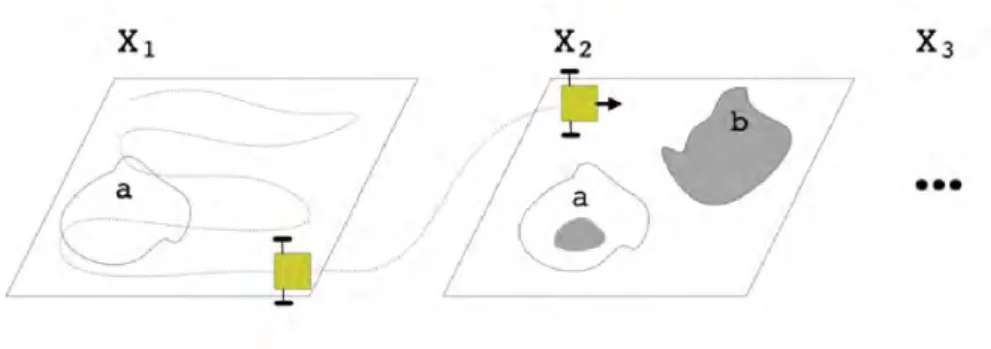
Environmental data are collected across time as well as space. A monitoring net-work (e.g., a netnet-work of meteorological stations) on which data are collected at reg-ular intervals, say every day or every week. With the introduction of geographical location as a new dimension, spatio-temporal data are gaining popularity as a new form of environmental data representation.
Such complexity appears normally resulting from that environmental data which contains information of locations, time, and state of environmental condition (i.e., pollution level). Fig.2.5 shows an example of landscape image series with changes happening at different levels (e.g., individual, summary) collected periodically at different locations (Rasinmaki, 2003).
Consider the spatio-temperal characteristic of environmental data, the computa-tional analysis has to consider spatial dependence of monitoring stations, and that the observations from each monitoring site typically are not independent but form a time series. The challenges of computational environmental analysis include, (1) The different length of observations, missing data, whether conditions, inevitable
Figure 2.5: An example of spatio-temporal Data.
occasional failures, and open or close a monitoring site through the observation pe-riod in the corresponding stations makes huge problems in spatio-temporal data analysis; and (2) Environmental problems are often temporally rich in data, un-fortunately sporadic collected spatially. One major short-coming documented in the literature is the ineffective use of spatial data for computational environmental analysis.
2.3.3
Endless Data Stream
The environmental data is collected every hour or every 8-hours or every day de-pending on the responses from monitor set. The monitoring is conducted continu-ously possibly without end. For air quality monitoring, the chemical compositions SO2,N O2,O3,P Mxare recorded every day even every hour. For land use
observa-tion, the real-time satellites imagery is in a large size with high-resolution. In gen-eral, environmental data does not take the form of persistent relations, but rather arrives in multiple, continuous, rapid, time-varying data streams (Babcock, Babu, Datar, Motwani, & Widom, 2002).
In computational environmental analysis, these possibly unpredictable and un-bounded streams cause some fundamentally research problems. Traditional database management and analysis models are not designed for rapid and continuous load-ing of individual data items, and they do not directly support the continuous queries (Terry, Goldberg, Nichols, & Oki, 1992).
how-ever, minimizing the real-time uncertainties by recognizing and reducing possible errors rapidly and efficiently is a hard topic (Titov et al., 2005). Therefore, we ex-plore that the challenges on real-time data stream analysis are accuracy, speed and robustness.
2.3.4
Missing Data
In environmental research, missing data often happen, usually due to faults in data acquisition, insufficient sampling or measurement error caused by non-response and break-down of equipment, and external (technical) reasons (Junninen, Niska, Tuppurainen, Ruuskanen, & Kolehmainen, 2004). Problems of missing data arise in most environmental studies, an incomplete data leads to result that are different from those that would have been gained from a complete dataset (Hawthorne & Elliott, 2005).
In practice if missing data exists, standard identification algorithms cannot be applied directly to pollution prediction. The missing data often interrupt the trend of an environmental problem, training models therefore lose the smooth operation unexpectedly (Xue et al., 2005). In addition, few missing data can seriously mislead the interaction between pollutants in training a prediction model (H. Li, Robertson, & Jensen, 2005). Although there are many techniques exist to recover data with missing values, but it has been considered as no one is absolutely better than the others (Graham, 2009).
2.4
Conclusion
In this chapter, we discussed the mechanism of environmental data collection and discover relevant problems on data quality. Environmental surveying provides ac-curate chemical parameters in water/air/soil, but it is often not possible or imprac-tical to evaluate environmental condition in real time. Monitoring network uses flexible programmable equipment to take samples at fixed or variable time intervals, where the quality of data is highly influenced by many uncontrollable environmen-tal factors. Remote sensing monitors the land cover problems in a large area using high resolution photography, on which noise may appear in data as a consequence of ambient lighting, weather phenomena and limitations of the spectral resolution.
Thus, the quality of environmental data is highly affected by uncontrollable vironmental phenomena and unexpected equipment failure. For computational en-vironmental analysis, noise and missing samples may seriously impact the useful-ness of analysis model. In addition, environmental problems are all spatio-temporal
characteristic with data collected at different locations and at different time peri-ods. Therefore, the challenge of computational environmental analysis is to handle spatio-temporal data streams with noise and missing samples.
Chapter 3
Environmental Change Detection
Environmental changes with its accumulating effects eventually destroy our agri-culture, forest, dike etc., and even cause flooding. The detection of environmental change is a process of identifying differences in the state of an environmental phe-nomenon by observing it over times. Essentially, it builds the ability for us to quan-tify temporal effects using multi-temporal datasets, and issue early warning for a potential environmental problem. This chapter discusses environmental change de-tection with a focus on the environmental problems addressed by the thesis.
3.1
Introduction
Environmental changes include emergence of new pollutant, interaction between pollutants, changes of densities of pollutants and changes of pollution types and level. Well known environmental changes are global temperature changes, drink-ing water quality changes and land cover changes, which are caused by emission, sewage and storm-water disposal and urban expansion. Many potential issues may be brought in by such environmental changes.
One of those issues is pollution which has already become one of the most seri-ous concerns of humans, since health problems caused by pollution have increased rapidly. Usually, pollution can be categorized as air pollution, water pollution and soil/land pollution. Each of them poses a grave threat to human. For example, World Health Organization (WHO) estimated that air pollution kills at least 2.4 mil-lion people every year (WHO, 2002). Guardian (2008) indicates that air pollution from motor vehicles is the most serious factor leading to pneumonia related deaths. Water pollution has been suggested to be a major global problem as it is the leading cause of deaths and diseases worldwide (Larry, 2006). Larry (2006) accounts the 14,000 daily deaths due to water pollution in 2006. Similarly, soil / land pollution emits hazardous substances into the air and groundwater (Risk Assessment Guidance
for Superfund (RAGS), 2009), causing a series of issues, such as land surface losing,
desertification and deforestation. Therefore, it will be a significant and continuous challenge of controlling pollution.
Every environmental event starts from changes. Environmental changes indicate the beginning of pollutions and examine the effective of environmental protection strategies. For example, melting of the polar ice caps is caused by global tempera-ture changes. Global temperatempera-ture change is caused by increasing densities of car-bon dioxide, methane, chlorofluorocarcar-bons, ozone, and nitrogen oxides. A change of carbon dioxide density is caused by the density changes of burning carbon fu-els in the air. Using of natural gas creates methane. Chlorofluorocarbons density changes mean people are using CFCs-MDI. Ozone density changes because of the use of electrical appliances. Nitrogen oxides are from toxic emission. If people are aware of where and what environmental changes happen, many diseases can be avoided. Therefore, environmental change detection is considered as the first step of all environmental protection system.
According to the detection methods for different types of pollution, environmen-tal change detection is categorized as traditional discriminant methods and state-of-the-art methods. Traditional discriminant methods include manual methods and instrumental monitoring methods. State-of-the-art methods use mathematical mod-els to analyze the environmental changes. Recently, air pollution, water pollution, and land pollution are increasingly under observation by satellite images. Thanks to accurate radiometric calibration, satellite images can provide easy-to-use and cost-effective data(Chavez, 1996). To develop change detection methods based on satel-lite images are more popular. Thus, satelsatel-lite images change detection plays a very important role in environmental protection.
This chapter is organized as follows: In Section 3.2, we present the brief con-cepts of existing change detection methods and compare them from the literature. In Section 3.3, we propose new criteria for evaluating change detection methods. In Section 3.4, we introduce some applications of environmental prediction. Finally, a summary is provided in Section 3.5.
3.2
Computational Change Detection Methods
This section reviews change detection methods. Subsection 3.2.1 illustrates tradi-tional discriminant methods. Due to the lack of technology and understanding of pollutants at the early stage, traditional discriminant methods were the major en-vironmental change detection method. Since then our understanding of pollutants including types of pollutants and their complicated interactions has been greatly deepened. Thus statistical methods and mathematical models can be employed on environmental change detection methods, which is discussed in subsection 3.2.2. In the modern era, satellite images provide diversified and accurate information to
researchers, such as globe temperatures, color of sea and land cover changes. There-fore, the satellite images change detection has been widely applied on air, water and land pollution. Satellite image change detection methods are discussed in subsec-tion 3.2.3.
3.2.1
Traditional Discriminant Methods
Sampling prior to statistical applications in environmental monitoring is the most popular method for environmental change detection, especially for air pollutants and water pollutants detection. Before state-of-the-art method, sampling does not only collect data, also detects changes directly. It is used to identify specific ab-normal activity patterns in an observation. For example, pondus hydrogenii (pH) value in water represents the acidity or basicity of an aqueous solution (Longsworth, 1964). pH value at25oCin pure water is considered as 7.0. pH value is less than 7, water is in acidic condition, oppositely, pH value is greater than 7, water is in alkaline condition. Sampling method uses universal indicator components to eval-uate pH value and compare a series pH value in a specific area to detect changes of acidity-alkalinity in water.
Since sampling methods use chemical containers or lighting to detect pollutants, it is categorized into manual methods and instrumental monitoring methods.
Manual methods
Manual methods sample air pollutants, and measure the levels of pollutants in the air/water by a standard. Manual methods for air pollutants detection include pas-sive samplers, paper tape samplers and bubbler systems. It also detects pollutants from water such as porous ceramic cups detection method.
1. Passive samplers (Klanova et al., 2006) collect gaseous air pollutants onto a chemical container.
2. Paper tape samplers (Martinez et al., 2008) analyze gas samples by a special paper. Each pollutants are marked by a series of discrete spots on the paper. 3. Bubbler systems (Anderson et al., 1995) bubble the air by a special designed
solution. Laboratory analysts then study the resulting solutions.
4. Porous ceramic cups samplers (E. A. Hansen & Harris, 1975) observe water samples’ sorption, leaching, diffusion, and screening of phosphate ions on the cup walls.
Instrumental monitoring methods
Instrumental monitoring methods apply an instrument to measure, detect air/water pollutants through a quantitative chemical reaction.
Non-dispersive infra-red (NDIR), chemiluminescence, flame photometric ana-lyzers and suspended particulate monitoring methods for air pollutants for air pol-lutants detection and immunofluorescence assay for water polpol-lutants detection are the most popular detection methods at present. liquid chromatography-electrospray tandem mass spectrometry
1. NDIR (Fischer et al., 2000) is employed to measure the absorption peak of the pollutant molecule by light emitted from an infra-red source which is not dispersed.
2. Chemiluminescence (Loomis et al., 1999) determines the pollutant air compo-nent, likeN Ox, by chemical reactions through light.
3. Flame photometric analyzers (Dagan, 2000) take photos for air pollutants, like sulfur, detected from chemical reactions within a hydrogen-rich flame and nar-row light. The photos show capacities and types of air pollutants.
4. Suspended particulate monitoring methods (Pope et al., 2002) apply a high volume air sampler (an air sampling equipment) to collect particles (PM-10) from air, then calculate weight of particles.
5. IFA (Russell, Sampson, Schmid, Wilkinson, & Plikaytis, 1984) visualizes the distribution of the target molecule through samples by the specificity of anti-bodies to their antigen to target fluorescent dyes to specific biomolecule targets within a cell.
6. Liquid chromatography-electrospray tandem mass spectrometry (Hirsch et al., 1998) combines the physical separation capabilities of liquid chromatog-raphy with the mass analysis capabilities of mass spectrometry.
Traditional discriminant methods can be sumaried as (3.1) (Paavola, Ruusunen, & Pirttimaa, 2005)
∆t=|Xt−Xt−1|, (3.1)
where∆tis the difference,XtandXt−1represents the current value of the
param-eter and the lagged value respectively. The alarm of change is∆t≥T hV al,T hV al