arXiv:1901.05797v1 [cs.DS] 17 Jan 2019
Boolean matrix factorization meets consecutive ones property
∗
Nikolaj Tatti
†Pauli Miettinen
‡Abstract
Boolean matrix factorization is a natural and a popular tech-nique for summarizing binary matrices. In this paper, we study a problem of Boolean matrix factorization where we addition-ally require that the factor matrices have consecutive ones prop-erty (OBMF). A major application of this optimization problem comes from graph visualization: standard techniques for visual-izing graphs are circular or linear layout, where nodes are ordered in circle or on a line. A common problem with visualizing graphs is clutter due to too many edges. The standard approach to deal with this is to bundle edges together and represent them as rib-bon. We also show that we can use OBMF for edge bundling combined with circular or linear layout techniques.
We demonstrate that not only this problem is NP-hard but we cannot have a polynomial-time algorithm that yields a multiplica-tive approximation guarantee (unless P=NP). On the positive side, we develop a greedy algorithm where at each step we look for the best 1-rank factorization. Since even obtaining 1-rank fac-torization is NP-hard, we propose an iterative algorithm where we fix one side and and find the other, reverse the roles, and repeat. We show that this step can be done in linear time using pq-trees. We also extend the problem to cyclic ones property and symmetric factorizations. Our experiments show that our algorithms find high-quality factorizations and scale well.
1
Introduction
Matrix factorization is an immensely popular way of sum-marizing data as well as discovering signal from the data. While being useful, the interpretation and visualization of discovered factor matrices may be difficult. A popu-lar variant for factorizing binary matrices is a k-Boolean matrix factorization, which, essentially, summarizes the binary data as a union ofktiles, that is, submatrices full of 1s. However, visualizing such factorization is difficult
∗This is an extended version of the paper of the same name presented
in 2019 SIAM International Conference on Data Mining.
†University of Helsinki, Helsinki, Finland,
‡University of Eastern Finland, Kuopio, Finland,
[email protected]. Part of this work was done while the author was with MPI-INF, Saarbrücken, Germany.
as the discovered rows and columns can be any sets, and there is no insightful way of visualizing them all at once.
In this paper we considerk-Boolean matrix factoriza-tion such that the resulting matrix has a certain property: we can order the columns and the rows such that the matrix consists of union ofkcontiguoustiles. We do not know the order before-hand, and we discover the order as we also discover the factorization.
Our motivation for discovering such factorization is pri-marily due to easy exploration of the factorization: we can draw the factorization as ktiles. While in certain cases, such a constraint may be too restrictive, there are many set-tings, where this constraint comes naturally. As a specific example, consider visualizing graphs. A classic technique for visualizing a graph is using linear or circular layout, where the nodes are drawn on a line or circle, and they are connected with arcs. The most common problem with visualizing graphs is clutter due to too many edges. To combat the clutter, edges are often grouped, and drawn in ribbons (see Figure 3 for an example). The problem is to discover such ribbons and the node order, while minimiz-ing the error. We show that we can use matrix factorization on the adjacency matrix of a graph to find the order and the groups.
We show that the factorization we seek can be ex-pressed with consecutive ones property (C1P). Namely, we will look for factor matricesXandY whose columns can be shuffled such that each row has a form of
[0, . . . ,0,1, . . . ,1,0, . . . ,0]. We show that the problem
isNP-hard, even if k = 1, and it is inapproximable for
k >1. On the positive side, we propose a greedy algo-rithm that searches the factors in iterative manner. The search is done by first fixing a vector inXand finding the optimal counterpart inY, then fixing the vector inY and finding the optimal vector inX, and so on, until conver-gence. We show that we can find the optimal counterpart in linear time using pq-trees.
We also consider 3 extensions of this factorization: the first variant, cyclic decomposition, consists of allowing factors to “wrap around the border.” the second variant is specifically designed for symmetric matrices, while the last variant combines the two. Performing cyclic and sym-metric decomposition proves to be useful for cyclic layout of graphs.
The rest of the paper is organized as follows: We present preliminary notation and define the matrix factorization and the cyclic version in Section 2. We present the search algorithm in Section 3. The symmetric extensions are given in Section 4. Section 6 is dedicated to related work, and Section 5 is dedicated to experimental evaluation. Fi-nally, we conclude the paper with remarks given in Sec-tion 7. All proofs are given in Appendix A.
2
Preliminary notation and problem
definitions
We begin by presenting preliminary notation, and then present the two main problem definitions. Extended prob-lems are discussed in Section 4.
2.1
Notation
Given an n-by-k binary matrix A and a k-by-m binary matrixB, theBoolean matrix product A◦ B is defined element-wise as (1) (A◦B)i j = k Ü ℓ=1 aiℓbℓj .
The Boolean matrix sum of A ∈ {0,1}n×m and B ∈
{0,1}n×mis defined elementwise as(A∨B)
i j =ai j∨bi j.
To measure the distance between two binary matrices, we use thesquared Frobenius normof their (normal) dif-ference,kA−Bk2F. Notice that asAandBare both binary, this is the same as calculating the number of disagreements betweenAandB: kA−Bk2F={(i,j):ai j ,bi j}
.
We say that a binary matrixX has aconsecutive ones property(C1P) if its columns can be permuted such that each row has a form of[0, . . . ,0,1, . . . ,1,0, . . . ,0], that is, 1s form a contiguous interval. For the sake of presentation, we will also refer these matrices asunimodal.
We say that a binary matrix X iscyclicif its columns can be permuted such that each row has a form of [0, . . . ,0,1, . . . ,1,0, . . . ,0]or[1, . . . ,1,0, . . . ,0,1, . . . ,1].
2.2
Problem definitions
Next we will give our two main optimization problems.
Problem 1(Ordered BMF,obmf). Given a binary matrix
Dand an integerk ∈N, find two unimodal binary matrices XandYthat minimize the number of disagreements (2) D− (XT ◦Y)
2
F.
Problem 2(Cyclic Ordered BMF,cobmf). Given a binary
matrixDand an integerk∈N, find two cyclic binary
ma-tricesXandYthat minimize the number of disagreements (3) D− (XT ◦Y)
2
F.
The matrix Z = XT ◦Y given in Eq. 2 has another natural alternative characterization: the columns and the rows ofZ can be permuted such that the resulting matrix is a union ofkcontiguous tiles of 1s. Similarly, the matrix
Z =XT◦Y given in Eq 3 can be permuted such that the
resulting matrix is a union of kcontiguous tiles, but we also allow the tiles to wrap around the border.
Unsurprisingly, the problems are computationally infea-sible. First, we demonstrate thatobmfis difficult even if
k=1.
Theorem 1. Theobmfproblem isNP-hard, even ifk=1.
Our next result shows that not onlyobmfis difficult, but it is also impossible to approximate. To show this, it is enough to demonstrate that testing for zero-error solution is expensive.
Theorem 2. Deciding whetherobmfhas a zero-error
so-lution isNP-complete.
The proofs of these and other statements are given in Appendix A.
3
Iterative greedy algorithm
3.1
Greedy algorithm
As we saw in the previous section, not only the problem is NP-hard, we cannot construct any polynomial-time algo-rithm with a multiplicative guarantee. Hence, we need to
resort to heuristics. The most natural heuristic is a greedy heuristic, where given a(k−1)-sized factorization we look for ak-sized factorization by adding one row and one col-umn toXandY. Note that these rows need to be selected carefully such thatXandYremain unimodal, and we also need to maintain the permutation(s).
Unfortunately, Theorem 1 states that we cannot even find the best solution fork=1 in polynomial-time. Fortu-nately, we can solve quickly a subproblem, where we have fixed one side.
Problem 3(Ordered BMF step,obmfstep). Given a
bi-nary matrixDof sizen-by-mand two unimodal matrices,
X′of size k-by-n andY′of size (k−1)-by-m, find the decomposition XT ◦Y solvingobmfsuch that X = X′ andY is obtained by adding one new row toY′.
We can useobmfstepas follows. Assume that we have already found(k−1)-by-mmatrices X andY. We first extend X with a new row using a given seed, and find the optimal new row forY (strategy for such selection is given later using obmfstep. We fix the discovered row, and use obmfstepto find the corresponding row for X. Since we solve each step optimally, the error will never increase. We stop when the error stops decreasing. Note that we will need to provide a seed for the initial row inX. Here, we test several possible seedsS, and select the best. We experiment with several options in experiments, but the default is thatSis equal to all singleton columns. The pseudo-code for the algorithm is given in Algorithm 1.
The remainder of this section is about solvingobmfstep in linear time. Almost the same approach will also work for the cyclic version,cobmfstep; we will point the minute difference.
3.2
Expressing permutations with pq-trees
The complicated aspect of obmfstepis that we need to make sure that the new matrix is unimodal. Luckily, we can use pq-trees, a classic structure that allows us to ex-press every permutation for which a set of binary vertices remain unimodal. In this section we will give a brief review of pq-trees and the two main properties that are relevant to us.Assume that we are given a universeU; in our case this will be either rows or columns of the input matrix. A pq-tree is a tree with each leaf corresponding tou ∈ U.
Algorithm 1:Greedy iterative algorithm for
estimat-ingobmf. The algorithm takes as input the dataset, the desired dimensionk, and the seed setS used for selecting the first candidate for a column.
1 X←matrix of size 0-by-n;
2 Y←matrix of size 0-by-m; 3 foreachi=1. . . ,kdo
4 foreachs∈Sdo
5 c←s;
6 whileerror decreasesdo
7 r←best row for fixed columns[Y;c];
8 c←best column for fixed rows[X;r];
9 X← [X;r];
10 Y← [Y;c];
There are two types of non-leaf nodes, these types will dictate what permutations we can perform on the children. We can permute children of p-node in any order whereas the order of the children of q-node is fixed but we can flip the direction. The leaves of the permuted tree will then indicate an order. We will denote such orders byorder(T), whereT is the pq-tree.
Two seminal results are important to us. The first result states that there is a pq-treeTsuch thatorder(T)are exactly the orders under which a set of binary vertices remain unimodal.
Theorem 3(Booth and Lueker [3]). Given a universeU
andksetsSi ⊆U, there is a pq-treeT such thatorder(T)
are exactly the permutations ofUunder which eachSi is
contiguous.
The second result states that we can efficiently update the pq-tree.
Theorem 4(Booth and Lueker [3]). Assume that we have
a pq-treeT over a universeUand a setS ⊆T. LetPbe
the set of all permutations ofUwhereSis contiguous. If
order(T) ∩P,∅, then there is anO(|U|)-time algorithm
that constructs a treeT′such thatorder(T′)=order(T) ∩
P. Iforder(T) ∩P=∅, then the same algorithm detects a failure.
The detailed description of the algorithm for updating the pq-tree can be found in [3].
3.3
Finding the optimal row
In this section we describe the algorithm that solves obmf-step. Assume that we have a pq-treeT representing the permutations of columns inDallowed by the previously discovered rows inY′. When dealing with pq-trees it is notationally easier to deal with sets rather than with vec-tors. Naturally every binary vectorycan be represented
as a setS={i: yi=1}.
Let us defineUto be the column indices of D; these are exactly the leaves ofT. We say that a set S ⊆ U
is compatible with a pq-tree T, if there is an order in
order(T)whereS is contiguous. Obviously, compatible setsScorrespond exactly to suitable new rows inY.
We can expressobmfstepas an instance of the following problem.
Problem 4(optset). Given a universeU, weightsw(u)
for eachu ∈U, and a pq-treeT over the universeU, find a setSthat is compatible withT and maximizes the total weightÍ
u∈Sw(u).
Recall thatu ∈Ucorresponds to a column index ofD. Definew(u)to be the gain in the error-function if we were to useuin our new row forY. More formally, letxbe the
fixed counterpart inXfor the new row inY. Letpbe the number of ones inDat rowsxand columnuthat are not
yet covered by the previous factors. Letnbe the number of zeros inDat rowsxand columnuthat are not yet covered
by the previous factors. We definew(u)=p−n. Solving optsetwith these weights solvesobmfstep.
In order to solve cobmfstep, we solve optset using
w(u)=p−n, as above, yielding a set, sayS1. In addition, we also solveoptsetusingw(u) =n−p, yielding a set,
sayS2. Then, we use eitherS1orU\S2, whichever yields a better gain.
In order to solveoptset, we need an additional defini-tion: LetSbe a compatible set of a pq-treeT. If there is a permutation inorder(T)with the first or the last element inS, we callSaborder-compatibleset.
LetT be a pq-tree. To solveoptsetwe will compute 3 counters for a nodevinT, namely,inner(v),border(v), andtotal(v). The countertotal(v)corresponds to the total weight of leaves underv, while the counterinner(v) cor-responds to the bestSthat is compatible with the subtree starting atv. Finally,border(v)corresponds to the bestS
that is border-compatible with the subtree starting atv.
We should stress that, strictly by definition,inner(v)can represent an empty set, whereas total(v) and border(v) should be never empty, even if they produce a neg-ative value. Thus, inner(v) ≥ 0 but border(v) and
total(v)can have negative values. Moreover, it is possi-ble thatborder(v)represents every leaf ofv, in which case,
border(v)=total(v).
Naturally, we want to computeinner(r), whereris the root ofT. To obtain this value we compute each value iteratively, children first. We also maintain the lists of the children that were responsible for producing the optimal value. These lists are clear from the proofs of the following lemmata. This allows us to extract the optimalS.
First, note that computing total(v) is trivial since
total(v) = Íc∈ch(v)total(c). If v is a leaf-node, then
border(v)=total(v)andinner(v)=max(0,total(v)). The next two lemmata establish how to compute the counters for q-nodes.
Lemma 5. Let v be a q-node and let c1, . . . ,cℓ be its
children. Then
border(v)=max(x, y), where
x=max i border(ci)+ i−1 Õ j=1 total cj, y=max i border(ci)+ ℓ Õ j=i+1 total cj .
Lemma 6. Let v be a q-node and let c1, . . . ,cℓ be its
children. Then
inner(v)=max(x, y), where
x=max i inner(ci), y=max i<j border(ci)+bordercj + j−1 Õ ℓ=i+1 total(cℓ) .
Our next step is to compute the counters for p-nodes. For that we need to define the following helper function: given a nodevwe defineg(v)=border(v)−max(total(v),0). We will useg(v)in the next two lemmata describing on how to compute the counters for p-node.
Lemma 7. Let v be a p-node and let c1, . . . ,cℓ be its
children. Defineb=maxg(ci). Then
border(v)=b+
Õ
i
Note that since we require the set responsible for
border(v)be non-empty, it is possible thatborder(v)<0. This can happen only ifb <0 and every childwofvhas
total(w)<0.
Lemma 8. Let v be a p-node and let c1, . . . ,cℓ be its
children. Defineb1 andb2 be the top-2 values ofg(ci).
Then
inner(v)=max(x, y), where
x=max i inner(ci), y=max(b1,0)+max(b2,0)+ Õ i max(total(ci),0).
Note that using these lemmas every counter can be triv-ially solved in linear time, except forinner(v), wherevis q-node. To computeinner(v)in linear time, it is enough if we can solve bordercj+max i<j border(ci)+ j−1 Õ ℓ=i+1 total(cℓ)
inconstanttime for afixed j. Luckily, we can rewrite this function as border cj+ j−1 Õ ℓ=1 total(cℓ) ! +max i<j t(i,j), where t(i,j)=max i<j border(ci) − i Õ ℓ=1 total(cℓ) .
Leti(j)to be the optimalifor a fixedj. Since max i<j t(i,j)=max t(j−1,j)max i<j−1t(i,j) ,
we have eitheri(j)=i(j−1)ori(j)=j−1. If we were to
test each j consecutively, then this allows us to compute
i(j) in constant time: we simply compare the solution
i=j−1 to the best previous solutioni(j−1).
In summary, each counter of v can be computed in O(|ch(v)|). Thus we needO(ℓ), whereℓis the number of nodes inT. Sinceℓ∈ O(|U|), we can compute the counters inO(|U|)time, where|U|is the number of columns inD.
When computing the counters we also store which chil-dren were responsible for this value. Once we have com-puted inner(r), wherer is the root of the tree, we can backtrack to obtain the optimalS. This can be also done in linear time.
Computing the weights w in optset can be done in O(p)time, wherepis the number of 1s in the datasetD
of sizen-by-m. Consequently,obmfstepcan be done in O(p+n+m)time.
4
Symmetric decomposition
We now propose an extension for symmetric matrices.
4.1
Definition
If Dis symmetric (e.g. an adjacency matrix of an undi-rected graph), we have the following problem:
Problem 5(Symmetricobmf,obmfsym). Given a binary
matrixDand an integerk ∈N, find two binary matrices XandY such that[X;Y]is unimodal, that minimize the number of disagreements
(4) D− (XT◦Y) ∨ (YT◦X)
2
F.
We define similarlycobmfsym, a cyclic and symmetric variant ofobmf.
The unimodality condition in obmfsym states that we should be able to permute X and Y with the
same permutation so that the rows are in form of [0, . . . ,0,1, . . . ,1,0, . . . ,0].
Notice that we do not use the more common symmetric decompositionD ≈XT ◦X as this would lead to neces-sarily having the blocks around the diagonal.
4.2
Algorithm
The discovery algorithm for symmetric obmfis similar. Like with the regularobmf, we use a greedy algorithm as an iterative step for discovering new rows.
The first difference is that we maintain only one pq-tree, corresponding to the rows in bothXandY.
The second difference is that – asXT◦Y andYT ◦X
can have overlapping 1s – maximizing optsetdoes not necessarily produce the optimal row. Instead, we can show
that solvingoptset, with the weights as described in the previous section, minimizesD−XT◦Y
2 F+ D−YT◦X 2 F.
It follows easily that minimizing this function yields a 2-approximation for finding optimal counterpart row.
5
Experimental evaluation
In this section we study how well the algorithms from Sections 3 and 4.2 work with synthetic and real-world data. We denote the algorithms with the same names as the problems they are solving, and differentiate the algorithms from the problems via the font. That is,obmf
is the algorithm forobmf, and so on. The algorithms are implemented in C++, and we make the source code and synthetic experiments freely available.1
5.1
Resilience to Noise
We start by evaluating the algorithms’ resilience to noise. To that end, we synthesized random matrices of size 95× 95 with block structure (6 blocks of size 20×20 along the diagonal, with 5 overlapping rows and columns) and corrupted those matrices with flipping a varying amounts of entries. The amount of flipped entries varied from 0 % to 50 % (of total elements) and we compared the quality of the results to both the noise-free matrix and noisy matrix. The results are shown in Figure 1.
With lower leves of noise (35 % forobmfandcobmf
and 25 % for the symmetric variants), the reconstruction of the original data is more accurate. With higher levels of noise, the noise has destroyed so much of the structure that the algorithms start fitting to the noise only, with a clear reduction of the quality versus the original data.
It is also worth noticing thatobmfobtains exact decom-positions when the data has no noise; the other methods introduce a slight error even in these cases emphasizing their more complex setting.
5.2
Scalability
In this section we test how wellobmfscales to larger data sets and how well it benefits from multiple cores. These experiments were executed on a server with 40 cores of
1https://cs.uef.fi/~pauli/bmf/ordered_bmf/
Intel Xeon E7-4870 processors running at 2.4 GHz. The algorithm was compiled using GCC 8.1.0 and the parallel code uses the OpenMP library.
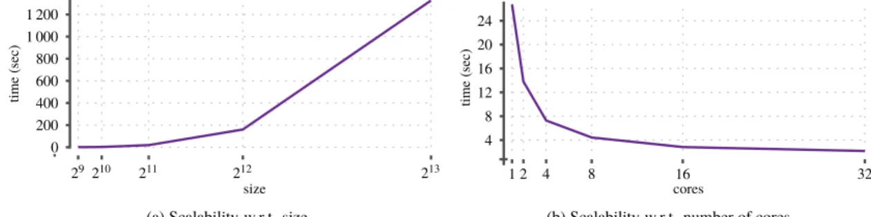
To test the scalability, we generatedn-by-nsquare ma-trices withn =2i fori =9, . . . ,13. All matrices have a density of approximately 24 %. The results are presented in Figure 2a.
The algorithm shows very good scalability over the full range, although it does get slower when the data size in-creases from 212to 213. It should be noted, though, that as the density is constant, the number of non-zeros in the matrices increases as the square of the matrix size. Hence,
obmfexhibits linear growth with respect to the number of non-zero elements.
Algorithm 1 is almost embarrassingly parallel over the different seeds vectors. Hence, we parallellized the test of different seeds, and tested how the algorithm behaves with increased number of cores. The results are in Figure 2b, where we can see that the speed-up is essentially linear up to 4 cores, slightly slower until 16 cores, and only marginal gains are available when increasing the number of cores to 32, indicating that at the algorithm has become memory bus constrained.
Overall, the experiments show that the algorithm scales very well, and is able to benefit from modern multi-core computers. We study further speed-up options later in Section 5.3.2.
5.3
Experiments with Real-World Data
We now turn to real-world data sets. We used six different real-world data sets, selected to offer a wide variety of different types of data. The data sets we used are as fol-lows.Les Misérablesis a standard benchmark data2of the characters of Victor Hugo’s novelLes Misérables. Paleois a palaeontological data3in the form of a locations-by-genera matrix, giving information where different fossiles have been found. Newsgroupsis a subset of the famous 20Newsgroups data4consisting four newsgroups and 100 terms. Terms the terms-by-terms co-occurrence matrix based onNewsgroups.Locationsis locations-by-locations matrix indicating mammal species co-location in the north-ern hemisphere: the data has a 1 in element(i,j)if
loca-2http://moreno.ss.uci.edu/data.html
3NOW 030717,http://www.helsinki.fi/science/now/
0 0.2 0.4 0 0.1 0.2 0.3 0.4 0.5 0.6 noise er ro r clean data noisy data (a)obmf 0 0.2 0.4 0 0.1 0.2 0.3 0.4 0.5 0.6 noise er ro r (b)cobmf 0 0.2 0.4 0 0.1 0.2 0.3 0.4 0.5 0.6 noise er ro r (c)obmfsym 0 0.2 0.4 0 0.1 0.2 0.3 0.4 0.5 0.6 noise er ro r (d)cobmfsym
Figure 1: Error as a function of noise. Here the error is the proportion of disagreements between the reconstructed matrix and either the noise-free or the noisy matrix. The decomposition was done using the noisy matrix.
29210 211 212 213 0 200 400 600 800 1 000 1 200 size ti m e (s ec )
(a) Scalability w.r.t. size
1 2 4 8 16 32 4 8 12 16 20 24 cores ti m e (s ec )
(b) Scalability w.r.t. number of cores
Figure 2: Scalability with respect to the size and number of cores.
tionsiand jhave at least five mammals in common. The data is based on the IUC Red List data.5 The final data set,
Mammals, contains a species-by-species co-inhabitation matrix.6 The data set properties are summarized in Ta-ble 1.
To the best of our knowledge, this is the first work to address the ordered Boolean matrix factorization prob-lem. To understand what kind of an effect the ordering constraint has to the reconstruction error, we compare our results with those of asso [15]. The asso algo-rithm is a well-known method for computing the standard Boolean matrix factorization. We used an
implementa-5http://www.iucnredlist.org/technical-documents/spatial-data
6Available for research purposes from the Societas Europaea Mam-malogica athttp://www.european-mammals.org
Table 1: Properties of real-world data sets. Rank indicates the rank used in the decomposition.
data rows cols % of 1s sym. rank
Les Misérables 77 77 8.57 Yes 10
Paleo 124 139 11.48 No 10
Newsgroups 100 348 6.30 No 10
Terms 100 100 48.54 Yes 10
Locations 3203 3203 8.42 Yes 50
Mammals 194 194 58.04 Yes 10
tion available from the author7and set the rank forasso
the same as for our algorithms, and used threshold values
τ={0.2,0.4,0.6,0.8}.
For symmetric data sets, we also computed the sym-metric Boolean factorization. This was done by first com-puting the standardXT◦Y factorization, and then testing whether XT ◦X orYT ◦Y gives smaller reconstruction error and using that one. This version ofassois denoted
assosym.
5.3.1 Reconstruction errors
We first compute the reconstruction errors for the various data sets. To facilitate the comparisons, we report the
relativereconstruction error kD−XT◦Yk2
F
kDk2F . The results of all datasets are given in Table 2.
In case of asymmetric decompositions,assois – as ex-pected, as its factor matrices are not restricted to unimodal or cyclic – almost always slightly better than eitherobmf
orcobmf. This difference is, however, very small in many
data sets (only 8 % inLes Misérablesand 0.50 % inPaleo). A remarkable exception is theMammalsdata, whereasso
is in fact worse than eitherobmforcobmf. As the data set is the densest of the ones we tested, it is possible that
assowas unable to obtain good candidates from it with the rounding thresholds we tried.
There is almost no difference betweenobmfandcobmf
in the terms of reconstruction error in these data sets. Usu-ally,obmfis on par or slightly better thancobmf, except again inMammals, wherecobmfis slightly better. The asymmetric data sets, PaleoandNewsgroups, cause the highest reconstruction errors at over 70 %. It should be noted, though, that also assohas similarly high errors with these data sets, indicating that they might not have strong Boolean low-rank structure.
In symmetric decompositions, the relationship between the ordered BMF algorithms andassois reversed, with
assosymbeing often the worse method (with the exception ofTerms). This is not very surprising, given thatassois not designed for symmetric decompositions. The errors are slightly worse than with the asymmetric algorithms, highlighting the complexity of finding the symmetric de-compositions.
5.3.2 Changing the seeds
In the above experiments, we used the columns as the seedsS for the algorithm (cf. Algorithm 1). This slows the algorithm down, as it has to attempt all of the potential seeds. In this section we study if we can improve the running time without hurting the reconstruction error by sampling only some of the columns for the seed setS.
In particular, we sampled 10 % of the columns uni-formly at random to create the seed set. As the algorithm scales linearly with the number of seeds, this provides an order of magnitude speed-up. To test the quality, we repeated the sampling ten times and report the average relative reconstruction errors and standard deviations in Table 3.
The first thing to notice in Table 3 are the low standard deviations; less than 3 % in almost all data sets. The reconstruction errors are also only slightly higher than those in Table 2; for instance,obmfwithPaleohas only 6 % higher error on average when using random sampling. In most cases the speed-up obtained by the sampling is significant compared to the loss in accuracy.
5.4
Visualizing the Graphs
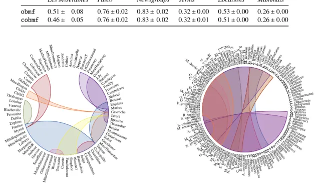
One of the motivations for the ordered BMF is that it al-lows the convenient visualization of the graphs using edge bundles (or ribbons) between nodes that are placed in a circle. In this section we explore some of these visualiza-tions and explain what we can learn from the respective data sets using them. In the following plots, the edge bun-dles and the ordering are obtained form the factorization. Further visualizations can be found in Appendix B.
The Les Misérables data: The visualization of the
Les Misérablesdata is presented in Figure 3. Most edge bundles form a circular segment indicating that all of the nodes under the segment are connected to each other (the characters appear in the same parts of the book). Some of the bundles are contained in other bundles, indicating important subset of characters. Multiple bundles intersect on a node at south-east of the circle calledValjean– the protagonist of the book.
TheMammalsdata:The second data set is the Mam-malsdata, in Figure 4. For a clearer visualization, we only consider 134 species that do not appear too frequently in the data, as such species are neighbours of every other
Table 2: Relative errors with asymmetric (left) and symmetric (right) algorithms on real-world data.
Les Mis Paleo News Terms Locations Mammals
obmf 0.36 0.71 0.74 0.32 0.40 0.26
cobmf 0.36 0.72 0.74 0.32 0.40 0.26
asso 0.33 0.71 0.72 0.29 0.34 0.26
Les Mis Terms Locations Mammals
obmfsym 0.40 0.35 0.48 0.27
cobmfsym 0.41 0.36 0.45 0.27
assosym 0.66 0.33 1.02 0.33
Table 3: Average relative errors and standard deviation with random columns as seeds for asymmetric algorithms on real-world data. Ten random samples.
Les Misérables Paleo Newsgroups Terms Locations Mammals
obmf 0.51± 0.08 0.76±0.02 0.83±0.02 0.32±0.00 0.53±0.00 0.26±0.00 cobmf 0.46± 0.05 0.76±0.02 0.83±0.02 0.32±0.01 0.51±0.00 0.26±0.00 Myriel N ap oleo n MlleB aptisti ne Mme Magloi re C ou ntes sD eLo G eb oran d C ham pte rcier C rav atte Coun t OldM an Laba rre V aljea n Mar guer ite Mm eDeR Isab eau Ger vais Tholomyes Listolier Fameuil Blacheville Favourite Dahlia Zephine Fantine M m eThe nard ier Thenardier C o se tt e Javert F au ch el ev en t B am atab ois Per pet ue S im p lice Sca uffl aire W om an1 Jud ge C h am pm ath ieu B re vet C heni ldie u C oche pa ille Pon tmer cy Bo ula tru elle Eponine An zelm a Wo man 2 Mo ther Inn oce nt G ri b ier Jon d re tte Mm eBurgon Gavroche Gil len orm and M agn o n Mll eG ille norm and M m ePo n tm er cy M lleV aub ois LtG ille norm and Marius Bar ones sT Mabeuf Enjolras Combef erre Prouva ire Feuil ly Cour feyra c Baho rel Bossuet Joly Gra ntai re M oth erP luta rch Gueul em er
BabClaqetuesous Mon tparnasse T ouss ai nt Child1 Child2 Brujon Mm eHuc helo up
Figure 3: Visualization of theLes Misérables data with the ribbons and ordering fromcobmf.
species in graph. The edge bundles in Figure 4 are es-sentially rotating around the middle. This probably corre-sponds to the change of fauna when moving from north to south. The change is gradual, hence two consecutive edge bundles have a significant overlap, but over longer distance, the change in the fauna becomes more obvious and the edge bundles are more disjoint. This gives a good intuition about the structure of the data.
A. minous A. alces A. lagopu s A. l ervi a A.agrariu s A . alp ic ola A . m y st ac in u s A . ura le nsis A . sa pidus A . alg ir us A. getulus A. a xis B. b onas us C. e ryth raeu s C. finlaysonii C . au re u s C .ae gag rus C . ib ex C .p y ren ai ca C. cana densis C.fib er C . nip pon C. niv alis C. rufoc anus C. rutilus C . m ig ra to riu s C. c ric etus C. canariensis C. leu cod on C. osorio C. r ussu la C. s icul a C. zimmerm anni D . bog dano vi D. n it edu la E. bottae E.ni lsson ii E. barbatus E . co n co lo r G .p yre n ai cus G . gen etta G. gulo H. grypus H. a urop unct atus H . ich n eum on H. inermis H. c rist ata
L. lemmus L. cape
nsis L. ca str ov iejo i L.co rsic anu s L. g ran aten sis L. t imid us L.lynx L . p ar dinu s M.syl vanus M.ruf ogris eus M. m arm ota M. tr istram i M . n ew to n i M. bavaricus M . c abre rae M . duo decim costa tus M . felten i M . g erbe i M .g u en th eri M . lu sitan icus M .m u ltip lex M.oec onom us M. rossiaem eri... M. sav ii M . subte rraneu s M. tatricus M . thom asi M. mo n ach u s M. ree vesi M . m ac edo n icu s M. m usculus M . sp icilegus M . spretu s M. evers manii M. l utre ola M. v ison M. c oy pus M . ro ac h i M. schisticolor M. b rand ti M. cap acci nii M. dasyc neme N .le u cod on N.az oreu m N. lasi opte rus N.pr ocyo noide s O. rosmarus O. virginianus O. z ibet hicu s O. moschatus P. groenlandica P. hispida P. vitulina P.m ader ensis P.te neriff ae P. lotor P. volans R. tarandus R .b la sii R. meh ely i R . p yren aica R. rup icapra S . an o m al us S.ca roli nen sis S.be tulin a
S. subtiS. alpinuslis
S. caecutiens S.co ron atu s S. grana rius S. isodon S. minutissim us S. sam nit icu s S .g ra ecu s S. cite llus S. suslicus S.et rusc us S. flo rid anu s T. te nio ti s T . c aeca T.oc ciden talis T. rom ana T. stankovici T. sib iricu s U. m ariti mus V. m urin us V. p ereg usn a
Figure 4: Visualization of the Mammals data with the ribbons and ordering fromobmf.
6
Related Work
Boolean matrix factorization(BMF) has received increas-ing interest in the data analysis community [2, 9–17], prov-ing to be a versatile tool for analyzprov-ing Boolean matrices. Many different algorithms have been proposed, includ-ing algorithms based on candidate creation and selection [12, 15], proximal alternations [10], and message passing [16], to name but a few. It has also found applications in diverse fields, such as bioinformatics [5], information
extraction [4], and lifted inference [18]. To the best of our knowledge, however, the ordering constraint is not studied in earlier work related to Boolean matrix factorization.
Tilingdatabases [6] can be seen as a restricted version of BMF, where the factorization cannot express any 0s as 1.
Geometric tiling[8] is a variation thereof, where the tiles have to be consecutive. The main difference to our work is a different optimization function, [8] uses log-likelihood, and that it assumes that the order is already given, for example, by spectral ordering, whereas we discover the order on the fly.
A binary matrix has theconsecutive ones property(C1P) if its columns can be permuted so that all rows have all 1s consecutively. The pq-trees can be used to check for the C1P [3] and Atkins et al. [1] propose spectral ordering algorithm. The spectral ordering approach is used in [8] to permute the data for finding the geometric tiles.
7
Conclusions
Ordered Boolean matrix factorization (obmf) and its varia-tions (cobmf,obmfsym) are restricted versions of Boolean matrix factorization, requiring the factors to have the con-secutive ones property (or be cyclic, in case of cobmf). This restriction facilitates the interpretation of the factor-ization, in particular in the case of the edge bundle visu-alizations of graphs, as we saw in Section 5.4. On the other hand, the restriction yields higher reconstruction er-rors, though our experiments show that the difference to state-of-the-art Boolean matrix factorization algorithm is usually very small.
In this paper we laid the theoretical foundations of the obmfproblem and its variations, and proposed algorithms based on the pq-trees. An important part of the proposed algorithm is the choice of the seed vectors. In this paper, we mostly used all columns of the data as the seed, though the experiments in Section 5.3.2 show that sampling the columns could work equally well. An interesting question for the future is whether other methods for selecting the seeds would yield better reconstruction errors.
In the problem setting of this paper, the user provides the rank of the decomposition and the goal is to minimize the reconstruction error over the rank-kobmf decomposi-tions. A common variant in the Boolean matrix factoriza-tion world is to make the rank a free variable and replace
the target function with measure that penalizes for higher ranks (see, e.g. [10, 12, 14]). TheMinimum Description Lengthprinciple is a common approach. The ordered na-ture of our factor matrices could help with finding more efficient MDL decompositions, as the factor matrices are easier to compress using run-length encoding or similar approaches.
References
[1] J. E. Atkins, E. G. Boman, and B. Hendrickson. A Spectral Algorithm for Seriation and the Consecutive Ones Problem. SIAM J. Comput., 28(1):297–310, 1998.
[2] R. Bělohlávek and V. Vychodil. Discovery of optimal factors in binary data via a novel method of matrix decomposition. J. Comput. Syst. Sci., 76(1):3–20, 2010.
[3] K. S. Booth and G. S. Lueker. Testing for the con-secutive ones property, interval graphs, and graph planarity using pq-tree algorithms. J. Comput. Syst. Sci., 13(3):335–379, 1976.
[4] E. Cergani and P. Miettinen. Discovering relations using matrix factorization methods. InCIKM ’13, pages 1549–1552, 2013.
[5] G. Corrado, T. Tebaldi, G. Bertamini, F. Costa, A. Quattrone, G. Viero, and A. Passerini. PTRcom-biner: mining combinatorial regulation of gene ex-pression from post-transcriptional interaction maps.
BMC Genomics, 15(1), Apr. 2014.
[6] F. Geerts, B. Goethals, and T. Mielikäinen. Tiling databases. InDS ’04, pages 278–289, 2004. [7] N. Gillis and S. A. Vavasis. On the Complexity of
Robust PCA andℓ1-norm Low-Rank Matrix Approx-imation.arXiv, 2015.
[8] A. Gionis, H. Mannila, and J. K. Seppänen. Geomet-ric and Combinatorial Tiles in 0–1 Data. InPKDD ’04, pages 173–184, 2004.
[9] S. Hess and K. Morik. C-SALT: Mining Class-Specific ALTerations in Boolean Matrix Factoriza-tion. InECMLPKDD ’17, pages 547–563, 2017. [10] S. Hess, K. Morik, and N. Piatkowski. The
PRIMP-ING routine—Tiling through proximal alternating linearized minimization. Data Min. Knowl. Discov., 31(4):1090–1131, May 2017.
[11] S. Karaev, P. Miettinen, and J. Vreeken. Getting to Know the Unknown Unknowns: Destructive-Noise Resistant Boolean Matrix Factorization. InSDM ’15, pages 325–333, 2015.
[12] C. Lucchese, S. Orlando, and R. Perego. A Unifying Framework for Mining Approximate Top-k Binary Patterns. IEEE Trans. Knowl. Data Eng., 26(12): 2900–2913, Dec. 2013.
[13] S. Maurus and C. Plant. Ternary Matrix Factoriza-tion: problem definitions and algorithms.Knowl. Inf. Syst., 46(1):1–31, Jan. 2016.
[14] P. Miettinen and J. Vreeken. MDL4BMF: Minimum Description Length for Boolean Matrix Factoriza-tion. ACM Trans. Knowl. Discov. Data, 8(4):–31, Oct. 2014.
[15] P. Miettinen, T. Mielikäinen, A. Gionis, G. Das, and H. Mannila. The Discrete Basis Problem. IEEE Trans. Knowl. Data Eng., 20(10):1348–1362, Oct. 2008.
[16] S. Ravanbakhsh, B. Póczos, and R. Greiner. Boolean Matrix Factorization and Noisy Completion via Mes-sage Passing. InICML ’16, 2016.
[17] T. Rukat, C. C. Holmes, M. K. Titsias, and C. Yau. Bayesian Boolean Matrix Factorisation. InICML ’17, pages 2969–2978, July 2017.
[18] G. van den Broeck and A. Darwiche. On the Com-plexity and Approximation of Binary Evidence in Lifted Inference. In NIPS ’13, pages 2868–2876, 2013.
A
Proofs
Proof of Theorem 1. In this case, we are looking for a decomposition of formatD≈xTy, whereD∈ {0,1}n×m, x ∈ {0,1}n, andy ∈ {0,1}m. Notice that (i) whether
we use normal or Boolean algebra does not matter in this case; and (ii) we can always find the ordering after we have found the decomposition, as we only need to order the vectorsxandy. But this problem, therank-1 binary
matrix factorizationproblem, is known to be NP-hard [7],
finalizing the proof.
Proof of Theorem 2. The decision problem is obviously in NP.
We prove the hardness by reduction fromHamilton path, where we are given a graphG=(V,E)and asked whether there is a hamiltonian path, that is, a path visiting every vertex exactly once.
Assume that we are given a graphG =(V,E)withn
vertices andmedges. Assume that we have some arbitrary order on the vertices V = v1, . . . , vn, and on the edges
E =e1, . . . ,em.
Let us define D first. The dataset will be of size (n+m+1)-by-(3m+1). To define the matrix, we split the rows in two parts R =r1, . . . ,rn andS = s0, . . . ,sm,
containing respectivelynandmrows. Similarly, we split the columns in 3 parts, X = x1, . . . ,xm,Y = y1, . . . , ym,
Z=y0, . . . , ym.
The 1s inDare as follows. for each edgeeℓ=(vi, vj), we
set the cells(ri,xℓ) (rj,xℓ) (ri, yℓ) (rj, yℓ)to be 1. For two
adjacent edgeseℓandeℓ+1, we set the cells(sℓ, yℓ) (sℓ,zℓ)
(sℓ,xℓ+1). Finally, we set(s0,x1), (s0,z0), and (sm, ym),
(sm,zm)to be 1. The remaining values are 0.
We argue that there is a zero-error solution forobmf using k =3m−n+2 if and only there is a hamiltonian path.
Let us prove the easy direction: assume that there is a hamiltonian path. To that end, let us permute the rows and columnsDsuch that the factor matrices do not have gap zeros. PermuteDas follows: Set the column order as
z0,x1, y1,z1,x2, y2, . . .. Order the rows inRaccording to
the hamiltonian path, followed by the rows inS. We denote the resulting matrix byD′. There is a zero-solution if the ones inD′are a union ofkcontiguous blocks. Thekblocks are as follows: m+1 blocks covering individual rows in
S,n−1 blocks covering edges along the hamiltonian path (this can be done since the corresponding rows inRand the corresponsding columns inXandYare adjacent), and 2(m−n+1)blocks to cover the remaining edges, 2 blocks per edge. This covers all 1s usingm+1+n−1+2(m−n+1)=
kblocks.
Let us prove the other direction. Assume that there is zero-error solution, and letD′be the permuted version of
Dwith no gap zeros. Then the ones inD′must be a union ofkcontiguous blocks. For a column indexi, we definefi
to be the number of blocks started at theith column. Let us also definegi to be the number of blocks ended atith
columns. Trivially,Í
i fi +gi =2k.
We say that an edge(vi, vj) ∈ E isactiveifiandj are
Note that we have h ≤ n−1. Assume for a moment thath = n−1 and letw1, . . . wn be the vertices ordered
according to the order ofRinD′. Sinceh=n−1, we are forced to have(wi, wi+1) ∈E. This implies thatw1, . . . , wn
is a hamiltonian path.
We will now argue thath≥n−1.
Consider two adjacent columns atiandi+1. If none of the columns are inZ, then both columns contain 1 that is not in the other column. This forcesgi+fi+1 ≥2. The same argument holds if both columns are inZ.
Assume that thejth column is inXand(j+1)th column
is inZ. Assume thatgi + fi+1 =1. Leta andb be the
rows inRthat are active in thejth columns. SinceZdoes not have active rows, the block(s) coveringaandbmust terminate, and sincegi ≥1, we have only block, implying
thata and b are adjacent. The same result holds if we replaceXwithYor permute the order of the two columns. To summarize, ifgi+fi+1 =1, then eitherith or the(i+1)th
column corresponds to an active edge.
In addition, we must have f1 ≥ 1 andg3m+1 ≥ 1 as these columns have 1s. This leads to
2(3m−n+2)=2k= 3m+1 Õ i=1 fi+gi = f1+g3m+1+ 3m Õ i=1 fi+1+gi ≥2(3m+1) −2h,
proving the result.
Proof of Lemma 5. Let S be the optimal border-compatible set. Then there isi such that S is a union of the best border-compable set ofciand either the union
of all leaves inc1, . . . ,ci−1orci+1, . . . ,cℓ.
Proof of Lemma 6. Let S be the optimal compatible set. ThenSis either included completely within one child, or there are indicesi < j such thatS is a union of the best border-compable sets ofci,cj, and the union of all leaves
inci+1, . . . ,cj−1.
Proof of Lemma 7. Let S be the optimal border-compatible set. Then there isi such that S is a union of the best border-compable set ofci and the union of all
leaves of some children.
Letwbe a child ofv, iftotal(w) ≥ 0, then having the leaves ofwinShas positive gain. LetPbe these children. The total gain corresponds of having these children is
Í
imax(total(v),0).
We need to transform one of the children to a partial. Letw be a child ofv. Iftotal(w) < 0, thenv < P and addingw will have a gain ofborder(w). Iftotal(w) ≥0, thenv ∈P, and transformingwfrom a fully-covered node to a partial node will have a gain ofborder(w) −total(w). In summary, the gain is equal tog(w). Thus, selecting the vertex with the maximalg(w)should be the partial child
inS.
Proof of Lemma 8. Let S be the optimal compatible set. ThenSis either included completely within one child, or
Sis a union of some children and possibly up to two of the best border-compable sets for someci andcj.
Letwbe a child ofv, iftotal(w) ≥ 0, then having the leaves ofwinShas positive gain. LetPbe these children. The total gain corresponds of having these children is
Í
imax(total(v),0).
As shown in the proof of Lemma 7, b1 andb2 corre-spond the top-2 border-compatible sets. It may happen thatb1orb2are negative, in which case we simply do not add them toS. Thus the total gain of border-compatible sets is max(b1,0)+max(b2,0).
B
Further Visualizations
Here we present for theTermsandLocationsdata sets.
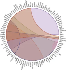
TheTermsdata The visualization of theTermsdata, in Figure 5, is markedly different from Figure 3. Here, most bundles overlap each other. This indicates that many of these terms are used together in different posts. Yet, we can also identify specialized groups of terms. At the left of Figure 5, we have a blue bundle, frommissiontonasa, that contains terms used when discussing space programs. This overlaps with a larger orange bundle, from chipto
tap, containing terms related to cryptography.
TheLocationsdata For theLocationsdata, in Figure 6, we cannot print any labels, as the data consists of 3203 geographical locations. For these results, we did a rank-10 decomposition. Most of the edge bundles again form
algo rith m nsa traffi c govern encr ypt kei clippe r secu r access escr ow cry pto gra ph i peopl sch em e enfo rc public system chip secr et comput p riv ac i effect cost agre faith pat d o cto r trust st er n li g h t den d ev ic d ecry pt w iret ap cryp to word pg ptap truth accept m ed sin space love nasa man christian christ god p hy sici an dis eas die t p atie nt teach m edic medic in infect foo d sym ptom tre atm ent pain syndrom clinic diagnos he nri etern speak toro nto bless fl ig ht rutger mission m oon spacec raft lunorbarit zoospence r lau nch shuttl solar prb heaven religi on vehicl satellit passa g gene va jesu chur ch clh bibl bibl ic holi cath ol ath o doct rin scri ptu r go spel jew rom an sp ir it
Figure 5: Visualization of theTermsdata with the ribbons and ordering fromobmf.
segments along the edge of the circle, corresponding to locations with similar fauna. Few larger edge bundles cover most of these locations, as well, corresponding to more general biospheres. In this figure, many nodes have no edges drawn. This indicates that they were not part of any significant quasi-clique.
Figure 6: Visualization of the Locations data with the ribbons and ordering fromobmf.