Localization Using Convolutional Neural Networks
Author: Shannon D. Fong
Advisor: Professor John Seng
Senior Project
Spring, Fall 2018
Computer Engineering Department
Table of Contents
Table of Contents 1
Introduction 2
Problem Statement 2
Software 2
Tensorflow 1.10 & Keras 2.2.4 2
Python Data Creation 3
Keras Image Generator 4
Keras Callbacks 4 Fine-tuning VGG19 5 CNN Testing 6 Hardware 7 Bill of Materials 8 Lessons Learned 8 Conclusion 10 Referenced Works 13 Figure Citations 14 Appendix 1: Code 15
Data Preparation: get_frames.py 15
Model Operations: model_ops.py 18
Retrain Classifier: retrain_classifier.py 21
Introduction
With the increased accessibility to powerful GPUs, ability to develop machine learning algorithms has increased significantly. Coupled with open source deep learning frameworks, average users are now able to experiment with convolutional neural networks (CNNs) to solve novel problems. This project sought to create a CNN capable of classifying between various locations within a building. A single continuous video was taken while standing at each desired location so that every class in the neural network was represented by a single video. Each location was given a number to be used for classification and the video was subsequently titled locX, see Figure 2 for mapping to Building 14. These videos were converted to frames to train several well known CNNs using fine-tuning. Once the CNN was trained, it was verified against a set of test photos taken separately from the original training videos.
Problem Statement
While many CNN classifiers exist, there are not many examples of a classifier used to determine location. When combined with other CNN’s for object avoidance, a location classifier may be useful for navigating indoor environments without barcodes or other identifiers. This project seeks to:
1) Create and optimize a convolutional neural network capable of localizing corners and hallways of California Polytechnic State University (Cal Poly) Building #14 Offices 2) Make the code flexible such that it may be applied to other locations
Software
Tensorflow 1.10 & Keras 2.2.4
Tensorflow is an open-source machine learning library. Tensorflow has been widely adopted and allows for research and development of powerful neural networks. However, there is a steep learning curve to learning neural networks and the Tensorflow framework, so the Keras Python library was used instead. Keras is a Python API designed to streamline the neural network development process. It provides classes and functions that make it easier to develop neural networks rather than learning to program them. Keras supports several backends, TensorFlow, CNTK, Theano, and hardware including NVIDIA GPUs, Google TPUs, and OpenCL-enabled GPUs ( Why Use Keras) . Code may be shared across platforms and preferences while requiring little modification to be executed.
Keras also provides several popular models that have been pre-trained on data from ImageNet. These models are the basis for this project by providing well verified baseline networks. Several
network designs were utilized within this project, VGG16, VGG19, and InceptionV3. A comparison between VGG16 and VGG19 is visible in Figure 1. All three of these pre-trained networks were put through training to add some redundancy then the superior model could be chosen after several comparisons.
Figure 1. VGG16 & VGG19. Figure 2. Numbered locations and Resulting File Structure.
Python Data Creation
Python was used as the main programing language for this project due to the Keras API. As such, the image data for training was generated using various libraries in the program
get_frames.py. The videos of each location were extracted to train and validation frames using the open-cv library and placed into the structure in Figure 2. A snippet of the frame parser can be seen in Figure 3. In order to avoid frames that are identical being in training and validation, variable validation_skip sets number of frames to be discarded before and after each frame selected for validation. The validation split will need to be lowered as this variable increases in order to attain the proper split, it is now tuned by the code. Photos need to be manually resized to 480x270 after being extracted. Test photos should also be taken manually so that they are never seen by the network being trained except in coincidental circumstances.
Figure 3. Splitting Images Code.
Keras Image Generator
This Keras utility allows for two things: reduction in memory usage by loading image batches one at a time and real-time data augmentation. Reduction in memory usage is especially important when being run on a CPU only because machine memory may be filled up quickly. While it was not as big an issue for this project since the images were only 480x270, every increase in image size causes an exponential increase in memory usage. Real time data augmentation is useful for reducing overfitting. Overfitting is when the model memorizes the training data rather than learning generalizations resulting in bad validation results. Arguments are straightforward and can be added and removed, allowing rapid model improvement (Figure 4).
Image generators may be used with the function flow_from_directory(). Flow_from_directory() will take the input as a tree like structure (Figure 2) and convert all folders to their own class and generate the appropriate labels. The ‘categorical’ argument (Figure 4) converts the labels to one-hot encoded arrays. This built in one-hot encoding saves both time and potential error by not requiring manual one-hot encoding. Flow_from_directory also has several parameters that may be of interest such as saving of augmented images, color mode conversions(grey_scale, rgb, etc.), and automatic resizing of images using various algorithms under ‘interpolation’.
Keras Callbacks
Keras callbacks are executed at the end of each epoch. Two callbacks were used for this project, the early stopping and model checkpoint callbacks (Figure 5). Early stopping is used stop the
model if it stops making progress. This is important because given enough time the model may memorize the validation data rather than guessing the validation data based on the training data. The patience parameter dictates how many non-improvements the training should accept before stopping. Model checkpoint is useful for generating a history of weights. Using the monitor and mode arguments it can be instructed to save when a parameter improves. In this project, it was used to save whenever the validation loss improved.
Figure 4. Datagenerator and flow.
Figure 5. Checkpoints.
Fine-tuning VGG19
Since there are many excellent CNNs with high accuracies, the decision was made to fine tune a few CNNs instead of attempting to develop a new one. As mentioned above, the VGG19
network was selected after several training sessions showing higher test accuracies than the other networks. In order to fine-tune the model, the fully connected (FC) layers of this model was removed and a simple 256 neuron FC layer and 9 neuron softmax output-layer were added in their place. The network was originally taking the output of the model and feeding that into the fully connected layer. This achieved acceptable accuracy ~80%. Accuracy was improved by
incorporating the pre-trained model into the new network and freezing the bottom layers. By freezing the bottom layers, the weights for early generalizations, like curves and edges, are preserved while the more fine weights related to ImageNet photos will be modified to fit this dataset. Integrating the pre-trained model and freezing weights can be seen in Figure 6. This resulted in accuracy gains of several percent. Once fine-tuning these layers of the pre-trained model, using a GPU is recommended as one epoch may take several minutes to complete on a CPU.
Figure 6. Model with frozen layers.
CNN Testing
Testing was done on a set of images manually taken in the locations that were previously
recorded. Test set contained 140 images in the same folder structure seen in Figure 2. This setup allowed the use of an image generator and flow_from_directory with a batch size of 1. Batch size was set to 1 so that each image is loaded and processed individually. Getting a summary of the results is done using evaluate_generator and getting predictions is given by predict_generator. One prediction contains percentages for all classes, so the max value in a prediction is the guess for that image. Comparing the index of the max value vs. the images label, contained in
generator.classes, will determine if the prediction was accurate. If examination of weight improvement vs testing improvement is desired, model checkpoint saves all weight
improvements to weights_path. If testing with a different weight set then the one generated by the final epoch, set test_weights to the appropriate file path and run program with --predict_only True. Final CNN training results may be seen below in Figure 7. Figure 7 shows a curve
demonstrating a slightly slow learning rate with little visible overfitting or underfitting.
Figure 7. Slightly slow learning rate training.
Hardware
The hardware for this project may be broken into two sections. Originally, the programs were being run on a lubuntu 18 virtual machine that was given 6, 4.9 GHz cores and 12 gb of RAM. This was fine for using very small networks or networks which took the output of a trained CNN as the input to the fully connected layer. This did not work for CNNs that sought to retrain convolution layers. When even one set of convolutional layers was added, epoch time would sky rocket to several minutes. So in order to make a reasonable amount of progress, the hardware was transitioned to a physical computer with a GPU.
Figure 8. GeForce 980TI Specs.
The computer mentioned was a Windows 10 machine with a 980TI Graphics card (Figure 8). Keras will automatically run on a GPU if it is present, so it is only necessary to make the GPU Tensorflow compatible, or whichever backend is being used. This page contains all the necessary instructions https://www.tensorflow.org/install/gpu , but there were several installation issues. Namely, the following configuration ended up being the first one to work and was corroborated by several forum posts: Tensorflow V1.1, Keras V2.2, cuDNN V7.X.X, CUDA V9. CUDA V10 with Tensorflow V1.1 did not work for this Windows 10 machine. CUDA install verification worked properly however there seems to be an incompatibility with Tensorflow V1.2.
Bill of Materials
Component Specification Size/Quantity Price
CPU Intel i7-8700K 1 $369.00
GPU MSI 980TI 1 $392.00
Motherboard ASUS Maximus X 1 $239.00
RAM Corsair, ddr4 16gb (4 x 4gb) $214.99
Power Supply EVGA Supernova 750 p2 750 Watt $159.99
Storage Samsung 870 EVO 250gb $77.99
Total Cost $1452.97
* These components represent the hardware utilized and in no way reflect the minimum requirement to work on a CNN using Keras and Tensorflow. The CNNs were being run for a time on a VM with half as many cores and RAM.
Lessons Learned
Two of the harshest lessons were the difficulty of gathering good data for training and the amount of time wasted running CNNs on a VM. In regards to data collection, originally photos were being taken manually from assorted angles to construct location classes. This resulted in < 50 photos of each location. Since this is clearly limited when it comes to training a CNN
augmentation was used to expand the dataset. Unfortunately, the augmentation scale ended up making some locations look like others resulting in poor training and subsequent testing
accuracy. The video approach was significantly superior resulting in a supply of 500+ frames in under 30 seconds of videotaping. Even excluding some frames to make validation frames unique resulted in ~40 validation frames and ~350 training frames.
Setup of the GPU to be CUDA enabled and usable by Tensorflow was a second significant pain point, but worth the effort. Tensorflow GPU install page links to all the latest versions of assorted software. Some of these links end up being compatible, and others do not. As previously
mentioned, CUDA V9 with cuDNN 7.X.X is necessary to operate properly with Tensorflow V1.1. The main Tensorflow page links to CUDA V10. If all the instructions for install are followed then it will appear to operate properly and all the CUDA samples will work. This setup did not work for running Keras with Tensorflow backend when used in this project. Also, the Windows paths set by the CUDA installer are wrong, this results in Tensorflow looking for a directory called CUDA which does not exist. Install the cuDNN in the path that the CUDA installer creates to fix the error and allow Tensorflow to locate the files.
Another lesson learned in this project was the necessity for meticulous little changes to CNNs. At the beginning, several parameters would be tweaked at once and significant improvements in accuracy would be seen. This was then not particularly useful as it is not obvious which
parameter had the most effect. Tweaking parameters such as learning rate, batch size, and number of frozen layers should all be done one at a time so their influence on the network may be properly examined. Without meticulous testing, good results may be gained but with no clear picture what to tune further in order to get even higher accuracies.
If this project were repeated, the number one thing that should be done differently is immediately setup Tensorflow to run on the GPU. While it may not seem like much at the start, those few seconds saved per epoch at the beginning add up. Also, it will need to happen anyway in order to process the more complex CNN’s weight trainings so it may as well be done from the start. While the setup was a pain, now that the compatibilities are listed there is no reason not to do the GPU setup first.
The other major improvement would be the use of videos for data collection from the start. Videos resulted in a 300+ frames in 30 seconds where the manual photo collection took much longer. With appropriate precaution, the videos can be split into a good testing and validation set with little to no duplicate data. Spending time manually taking photos proves equally accurate while providing significantly less data and requiring more time. Videos also add some real-time nature to the training data by occasionally blurring a frame. While this is not ideal for some things, in this case that data is useful. If this were implemented on a moving robot the occasional blurred frame due to a bump or sudden stop may occur so this skewed data may actual resolve momentary detection lapses in these cases.
Conclusion
This project was successful in training a CNN to classify locations within Building #14 Offices. Classifiers were able to achieve greater than 80% accuracy consistently with various parameters. Ideal parameters for this network are as follows: . Model with these parameters achieved an accuracy of . While improvements are surely possible with more data from varying weather conditions, an accuracy of __ would seem to be sufficient to qualify this project for successfully optimizing a CNN for localization.
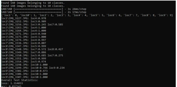
Three CNN’s were tested in unison while varying other parameters: VGG16, VGG19, InceptionV3(Figure 9, 10, 11). InceptionV3 testing accuracy achieved 77% while VGG19 achieved 87.8%. VGG16 showed its slightly smaller convolution network and came in at a testing accuracy of ~85.7%. This higher performance for the middle sized convolution network suggests that VGG16 was too simple and InceptionV3 too complex. InceptionV3 may have performed more memorization than generalization. Observing an even simpler network such as AlexNet may have yielded interesting results since VGG16 and VGG19 were comparable despite the deeper VGG19 structure. Location 7, 8, and 9 were often the failed test frames. Loc 5, 6, 7, and 8 were often mistaken for one another. Similarly, loc 1, 2, 3, and 4 were often confused and loc 8 and 9. These results are to be expected due to the symmetry of the building that was recorded. Loc 1-4, and loc 5-8 are in separate courtyards and 9-10 are both hallways. These results line up with expectations regarding error in this environment. Loc 3 images seem to exclusively error toward loc 4, this points to a possible lack of data for a certain angle of loc 3. In fact, a majority of the errors probabilities are greater than 80%. This seems to mean that each of these locations captured has a section with not enough data resulting in the other location video superseding based on the features the network learned.
Final program would also seem to be sufficiently flexible to satisfy the other objective of this project. Videos of locations may be quickly converted into classifications using get_frames.py. While test photos must be taken manually, this is a better practice to avoid biased testing data. While automatic resizing may have been preferred, manual resizing ensures the user briefly checks the resized images for distortions or other resizing issues. After manual resizing, the images can be sent through retrain_classifier.py in order to fine-tune the model.
Retrain_classifier allows for changing many parameters such as image dimensions, model to be trained, batch size, training depth, and others allowing users to tweak the network to fit their needs. The program provides succinct feedback and allows users to verify their trained weights sets against different test sets without retraining.
Figure 9. InceptionV3 Results
Figure 10. VGG19 Results
Figure 11. VGG16 Results
Referenced Works
Allanzelener. “Allanzelener/YAD2K.” GitHub , 2 July 2017, github.com/allanzelener/YAD2K.
Amaratunga, Thimira. “Using Bottleneck Features for Multi-Class Classification in Keras and TensorFlow.” Codes of Interest , 8 Aug. 2017,
www.codesofinterest.com/2017/08/bottleneck-features-multi-class-classification-keras.html.
Brownlee, Jason. “Multi-Class Classification Tutorial with the Keras Deep Learning Library.” Machine Learning Mastery , 2 June 2017,
machinelearningmastery.com/multi-class-classification-tutorial-keras-deep-learning-libra ry/.
J, Vijayabhaskar. “Tutorial on Using Keras flow_from_directory and Generators.” Medium.com , Medium, 12 Mar. 2018,
medium.com/@vijayabhaskar96/tutorial-image-classification-with-keras-flow-from-direc tory-and-generators-95f75ebe5720.
“Overfitting in Machine Learning: What It Is and How to Prevent It.” EliteDataScience , 7 Sept. 2017, elitedatascience.com/overfitting-in-machine-learning.
“Python | Program to Extract Frames Using OpenCV.” GeeksforGeeks , 15 May 2018, www.geeksforgeeks.org/python-program-extract-frames-using-opencv/.
Ruizendaal, Rutger. “Deep Learning #3: More on CNNs & Handling Overfitting.” Towards Data Science , Towards Data Science, 12 May 2017,
towardsdatascience.com/deep-learning-3-more-on-cnns-handling-overfitting-2bd5d99abe 5d.
Yu, Felix. “A Comprehensive Guide to Fine-Tuning Deep Learning Models in Keras.” A
Comprehensive Guide to Fine-Tuning Deep Learning Models in Keras (Part I) | Felix Yu , 8 Oct. 2016, flyyufelix.github.io/2016/10/08/fine-tuning-in-keras-part2.html.
Figure Citations
Cal Poly Seal“California Polytechnic State University.” Wikipedia , Wikimedia Foundation, 10 Dec. 2018, en.wikipedia.org/wiki/California_Polytechnic_State_University. Figure 1 https://tw.saowen.com/a/26ce2eceb89bda5409fc3c672277b4813356c37a7a028f8517d10cd81709 40ca Figure 2 https://afd.calpoly.edu/facilities/mapsplans/building/building%20014-0_frank%20e%20pilling% 20building.pdf Figure 4 https://www.geforce.com/hardware/desktop-gpus/geforce-gtx-980-ti/specifications
Appendix 1: Code
Data Preparation: get_frames.py
import cv2 import os import argparse import numpy as np import sys
# Function to extract frames
def parse_video(path, train, validate, test, split=0.15, fskip=1): global testCount vsplit = 1/split tsplit = vsplit * 4 #print(vsplit) validation_skip = 3
# Path to video file
vidObj = cv2.VideoCapture(path)
# Used as counter variable count = 0
imageNum = 0 trainCount = 0 vCount = 0
# checks whether frames were extracted success = 1
#Save current dir cdir = os.getcwd()
os.mkdir(train) os.mkdir(validate)
os.chdir(train) while success:
# vidObj object calls read # function extract frames success, image = vidObj.read()
# Saves the frames with frame-count if (count % fskip == 0):
quit = False
for img in os.listdir(test):
if np.array_equal(np.asarray(cv2.imread(img)), np.asarray(image)): print("Skipping duplicate frame")
quit = True break
#exclude duplicates, if found if quit == True: print("Skipped") continue imageNum += 1 if (imageNum % vsplit == 1): os.chdir(validate) skipCount = 0
while success and skipCount < validation_skip: prevImage = image
success, image = vidObj.read() skipCount += 1
vCount += 1
cv2.imwrite("frame%d.jpg" % vCount, prevImage) os.chdir(train)
skipCount = 0
while success and skipCount < validation_skip: prevImage = image
skipCount += 1 else:
trainCount += 1
cv2.imwrite("frame%d.jpg" % trainCount, image)
count += 1
#Back to parent dir os.chdir(cdir) # Driver Code if __name__ == '__main__': testCount = 0 parser = argparse.ArgumentParser() parser.add_argument("src", type=str,
help="filename containing videos") parser.add_argument("--dst", type=str,
help="filename containing videos") args = parser.parse_args()
vdir = os.getcwd() + "/" + args.src if args.dst != None: dst = args.dst else: dst = args.src + "Frames" videos = os.listdir(vdir) try: os.mkdir(os.getcwd() + "/" + dst + "") os.mkdir(os.getcwd() + "/" + dst + "/train") os.mkdir(os.getcwd() + "/" + dst + "/validate") os.mkdir(os.getcwd() + "/" + dst + "/test") wdir = os.getcwd() + "/" + dst except FileExistsError:
print("Remove destination directory or change dst") os.exit()
wdir = os.getcwd() + "/" + dst except:
print("An error Occured") os.exit()
print("Writing frames to %s" % wdir) test = os.getcwd() + "/" + dst + "/test" for video in videos:
parts = video.partition(".") try:
train = os.getcwd() + "/" + dst + "/train/" + parts[0] validate = os.getcwd() + "/" + dst + "/validate/" + parts[0] except:
print("An error Occured") os.exit()
parse_video(vdir + "/" + video, train, validate, test, 0.1, 2)
Model Operations: model_ops.py
from keras.preprocessing.image import ImageDataGenerator from keras.models import Sequential
from keras.layers import Dropout, Flatten, Dense from keras import applications
from keras.utils.np_utils import to_categorical from keras.optimizers import RMSprop
from keras.callbacks import EarlyStopping, ModelCheckpoint import argparse import cv2 import math import matplotlib.pyplot as plt import numpy as np import os import sys import importlib
from model_ops import *
#Intake model wiht no-top
#Create the Fine-Tuning Model w/last few layers unfrozen
def create_model(base_model, num_classes, dense_neurons=256, drop=0.7, unfreeze=5, final_act='softmax'): model = Sequential() model.add(base_model) model.add(Flatten()) model.add(Dense(dense_neurons, activation='relu')) model.add(Dropout(drop)) model.add(Dense(num_classes, activation=final_act))
for layer in base_model.layers[:-unfreeze]: layer.trainable = False
return model
def get_valid_gen(valid, dim, batch_size, shuffle=True): datagen_no_aug = ImageDataGenerator(rescale=1. / 255.0) validation_data = datagen_no_aug.flow_from_directory( valid, target_size=dim, batch_size=batch_size, class_mode='categorical', shuffle=shuffle) return validation_data
def get_train_gen(train, dim, batch_size): datagen_aug = ImageDataGenerator( rotation_range=10, width_shift_range=0.20,
height_shift_range=0.025, shear_range=0.15, fill_mode='nearest', rescale=1. / 255.0) #Create Generators train_data = datagen_aug.flow_from_directory( train, target_size=dim, batch_size=batch_size, #imagedir/whatever folder #This will eat up storage space
#save_to_dir="cscSengAllFrames2/augmented", class_mode='categorical', shuffle=True) return train_data '''
Function taken directly from
https://www.codesofinterest.com/2017/08/bottleneck-features-multi-class-classification-keras.ht ml
'''
def print_model_performance(history, model, data, steps): print("Evaluating model")
(eval_loss, eval_accuracy) = model.evaluate_generator( data, steps=steps, verbose=2)
print("[INFO] accuracy: {:.2f}%".format(eval_accuracy * 100)) print("[INFO] Loss: {}".format(eval_loss))
plt.figure(1)
# summarize history for accuracy
plt.subplot(211)
plt.plot(history.history['acc']) plt.plot(history.history['val_acc'])
plt.title('model accuracy') plt.ylabel('accuracy') plt.xlabel('epoch')
plt.legend(['train', 'test'], loc='upper left')
# summarize history for loss plt.subplot(212) plt.plot(history.history['loss']) plt.plot(history.history['val_loss']) plt.title('model loss') plt.ylabel('loss') plt.xlabel('epoch')
plt.legend(['train', 'test'], loc='upper left') plt.show()
Retrain Classifier: retrain_classifier.py
from keras.preprocessing.image import ImageDataGenerator from keras.models import Sequential
from keras.layers import Dropout, Flatten, Dense from keras import applications
from keras.utils.np_utils import to_categorical from keras.optimizers import RMSprop
from keras.callbacks import EarlyStopping, ModelCheckpoint import argparse import cv2 import math import matplotlib.pyplot as plt import numpy as np import os import sys import importlib
from model_ops import *
# dimensions of our images.
global img_width, img_height, final_weights, learn_rate global train_data_dir, validation_data_dir, tdir, save_dir global epochs, batch_size, val_batch_size
global unfreeze, dropout
train_data = get_train_gen(train, (img_height, img_width), batch_size)
validation_data = get_valid_gen(valid, (img_height, img_width), val_batch_size) #Gather Counts train_samples = len(train_data.filenames) num_classes = len(train_data.class_indices) validation_samples = len(validation_data.filenames) model = create_model(base_model, num_classes=num_classes, dense_neurons=256, drop=dropout, unfreeze=unfreeze, final_act='softmax') model.compile(optimizer=RMSprop(lr=learn_rate), loss='categorical_crossentropy', metrics=['accuracy'])
checkpoint = ModelCheckpoint(save_dir +'/model-{val_loss:.2f}.hdf5', monitor='val_loss', verbose=1, save_best_only=True, mode='min') earlyStop = EarlyStopping(monitor='val_loss', min_delta=0, patience=5, verbose=1, mode='auto') history = model.fit_generator(train_data, epochs=epochs, steps_per_epoch=int(math.ceil(train_samples / batch_size)), validation_data=validation_data, validation_steps=int(math.ceil(validation_samples / val_batch_size)),
verbose=2, shuffle=True, callbacks=[checkpoint, earlyStop]) model.save_weights(final_weights)
print_model_performance(history, model, validation_data, int(math.ceil(validation_samples / val_batch_size)))
def predict(image_path, base_model):
global learn_rate, final_weights, unfreeze, img_width, img_height datagen_no_aug = ImageDataGenerator(rescale=1. / 255.0) images = [] test = datagen_no_aug.flow_from_directory( image_path, target_size=(img_height, img_width), batch_size=1, class_mode='categorical', shuffle=False ) num_classes = len(test.class_indices)
test = get_valid_gen(image_path, (img_height, img_width), 1, False) model = create_model(base_model, num_classes=num_classes, dense_neurons=256, drop=dropout, unfreeze=unfreeze, final_act='softmax') model.compile(optimizer=RMSprop(lr=learn_rate), loss='categorical_crossentropy', metrics=['accuracy'])
model.load_weights(final_weights)
predict = model.predict_generator(test, steps=len(test.filenames), verbose=1)
results = model.evaluate_generator(test, steps=len(test.filenames), verbose=1) count = 0 correct = 0 error = 0 print(test.class_indices)
for prediction in predict:
if (np.where(prediction == max(prediction)) != test.classes[count]): error += 1
loc_count = 1
output = test.filenames[count] + ":" for val in test.class_indices:
if prediction[test.class_indices[val]] > 0.2:
output += " %s:%0.3f" % (val, prediction[test.class_indices[val]]) loc_count += 1 print(output) else: correct += 1 count += 1 count = 0
print("Overall Test Statistics:") for name in model.metrics_names:
print("%s: %f" % (name, results[count])) count += 1
cv2.destroyAllWindows()
# python retrain_classifier.py --epochs 100 --model VGG16 --freeze_layers 6 # cscSengAllFrames2 &&
# cscSengAllFrames2 &&
# python retrain_classifier.py --epochs 100 --model InceptionV3 --freeze_layers 6 # cscSengAllFrames2 &&
# python retrain_classifier.py --epochs 100 --model VGG16 --freeze_layers 6 # cscSengAllFrames2 --predict_only True &&
# python retrain_classifier.py --epochs 100 --model VGG19 --freeze_layers 6 # cscSengAllFrames2 --predict_only True &&
# python retrain_classifier.py --epochs 100 --model InceptionV3 --freeze_layers 6 # cscSengAllFrames2 --predict_only True
# Driver Code if __name__ == '__main__': parser = argparse.ArgumentParser() parser.add_argument("src", type=str, help="Direfctory to be processed")
parser.add_argument("--epochs", type=int, default=50, help="Number of epochs")
parser.add_argument("--val_batch_size", type=int, default=8, help="Val batch size to use")
parser.add_argument("--batch_size", type=int, default=16, help="Batch size to use")
parser.add_argument("--learn_rate", type=str, default=1e-5, help="Learning rate, default 1e-5")
parser.add_argument("--weights_path", type=str, help="Path to save weights too")
parser.add_argument("--test_weights", type=str, help="Weights file to use for testing")
parser.add_argument("--img_height", type=int, default=270, help="Image height, default 270")
parser.add_argument("--img_width", type=int, default=480, help="Image width, default 480")
parser.add_argument("--model", type=str, default='VGG19',
help="Which model to train with VGG16, VGG19, InceptionV3")
parser.add_argument("--predict_only", type=bool, default=False, help="Only Run Predictions")
parser.add_argument("--freeze_layers", type=int, default=5, help="Number of layers to NOT freeze")
parser.add_argument("--dropout", type=float, default=0.7, help="Dropout rate") args = parser.parse_args() if (args.src == None): args.print_help() sys.exit()
# dimensions of our images.
img_width, img_height = args.img_width, args.img_height unfreeze = args.freeze_layers dropout = args.dropout learn_rate = args.learn_rate epochs = args.epochs batch_size = args.batch_size val_batch_size = args.val_batch_size base_dir = args.src
train_data_dir = base_dir + '/train' validation_data_dir = base_dir + '/validate' tdir = base_dir + "/test"
if args.weights_path != None:
save_dir = os.getcwd() +"/" + args.weights_path + "/"
else:
try:
os.mkdir(save_dir)
print("Weights saved to %s" % save_dir); except:
#Do nothing
print("Weights saved to %s" % save_dir); if args.test_weights != None: final_weights = args.test_weights else: final_weights = save_dir+'/final_weights.h5' if args.model == 'VGG16':
base_model = applications.VGG16(include_top=False, weights='imagenet', input_shape=(img_height, img_width, 3))
elif args.model == 'InceptionV3':
base_model = applications.InceptionV3(include_top=False, weights='imagenet', input_shape=(img_height, img_width, 3))
elif args.model == 'InceptionResNetV2':
base_model = applications.inception_resnet_v2(include_top=False, weights='imagenet', input_shape=(img_height, img_width, 3))
else:
base_model = applications.VGG19(include_top=False, weights='imagenet', input_shape=(img_height, img_width, 3))
#Retrian
if (not args.predict_only):
retrain_model(train_data_dir, validation_data_dir, base_model)
print("Testing on %s" % tdir) #Run predictions and display predict(tdir, base_model) cv2.destroyAllWindows() #@misc{chollet2015keras, # title={Keras},
# author={Chollet, Fran\c{c}ois and others}, # year={2015},
# howpublished={\url{https://keras.io}}, #}