Multi-view Data Analysis

(1)

6/2

019

UA

N

Q

UN

C

AO

M

ult

i-v

iew

D

ata

A

na

ly

sis

Multi-view Data Analysis

GUANQUN CAO

(2)

Tampere University Dissertations 6

GUANQUN CAO

Multi-view Data Analysis

ACADEMIC DISSERTATION To be presented, with the permission of

the Faculty Council of the Faculty of Computing and Electrical Engineering of Tampere University of Technology,

for public discussion in the Auditorium TB109 of Tietotalo Building, Korkeakoulunkatu 1, Tampere,

(3)

Tampere University, Faculty of Information Technology and Communication Sciences Finland

Supervisors Moncef Gabbouj, Professor Alexandros Iosifidis, Associate Professor

Tampere University Aarhus University

Finland Denmark

Pre-examiners Guoying Zhao, Professor Abdulmotaleb El Saddik, Professor

University of Oulu University of Ottawa

Finland Canada

Opponent Gaurav Sharma, Professor

University of Rochester USA

The originality of this thesis has been checked using the Turnitin OriginalityCheck service.

Cover design: Roihu Inc.

ISBN 978-952-03-0967-1 (print) ISBN 978-952-03-0968-8 (pdf) ISSN 2489-9860 (print) ISSN 2490-0028 (pdf) http://urn.fi/URN:ISBN:978-952-03-0968-8 PunaMusta Oy Tampere 2019

(4)

Abstract

Multi-view data analysis is a key technology for making effective decisions by leveraging information from multiple data sources. The process of data acquisition across various sensory modalities gives rise to the heterogeneous property of data. In my thesis, multi-view data representations are studied towards exploiting the enriched information encoded in different domains or feature types, and novel algorithms are formulated to enhance feature discriminability. Extracting informative data representation is a critical step in visual recognition and data mining tasks. Multi-view embeddings provide a new way of representation learning to bridge the semantic gap between the low-level observations and high-level human comprehensible knowledge benefitting from enriched information in multiple modalities.

Recent advances on multi-view learning have introduced a new paradigm in jointly mod-eling cross-modal data. Subspace learning method, which extracts compact features by exploiting a common latent space and fuses multi-view information, has emerged proimi-nent among different categories of multi-view learning techniques. This thesis provides novel solutions in learning compact and discriminative multi-view data representations by exploiting the data structures in low dimensional subspace. We also demonstrate the performance of the learned representation scheme on a number of challenging tasks in recognition, retrieval and ranking problems.

The major contribution of the thesis is a unified solution for subspace learning methods, which is extensible for multiple views, supervised learning, and non-linear transformations. Traditional statistical learning techniques including Canonical Correlation Analysis, Partial Least Square regression and Linear Discriminant Analysis are studied by constructing graphs of specific forms under the same framework. Methods using non-linear trans-forms based on kernels and (deep) neural networks are derived, which lead to superior performance compared to the linear ones. A novel multi-view discriminant embedding method is proposed by taking the view difference into consideration. Secondly, a multi-view nonparametric discriminant analysis method is introduced by exploiting the class boundary structure and discrepancy information of the available views. This allows for multiple projecion directions, by relaxing the Gaussian distribution assumption of related methods. Thirdly, we propose a composite ranking method by keeping a close correlation

(5)

with the individual rankings for optimal rank fusion. We propose a multi-objective solution to ranking problems by capturing inter-view and intra-view information using autoencoder-like networks. Finally, a novel end-to-end solution is introduced to enhance joint ranking with minimum view-specific ranking loss, so that we can achieve the maximum global view agreements within a single optimization process.

In summary, this thesis aims to address the challenges in representing multi-view data across different tasks. The proposed solutions have shown superior performance in nu-merous tasks, including object recognition, cross-modal image retrieval, face recognition and object ranking.

(6)

Preface

The research presented in this thesis has been carried out at the Laboratory of Signal Processing, Tampere University of Technology (TUT), Finland, during 2012-2018. This thesis owes its existence to the help, support, and inspiration of many people. First and foremost, I would like to express my deepest gratitude to my supervisor, Prof. Moncef Gabbouj for his advice, support and patience over the years to make the thesis happen. Prof. Gabbouj has provided a wonderful environment which enables me to focus on the research work. His words of wisdom, critical thinking, and admirable personality conveyed through our discussions and meetings will benefit me in the long run.

I am indebted to Prof. Alexandros Iosifidis as my instructor, for his excellent guidance and continuous encouragement for my research work. I am very grateful for his precise instruction, relentless support, and careful review of my papers and thesis. I wish to express my gratitude to Dr. Ke Chen, whom I had the initial discussion about multi-view data analysis with. His inspiration and support have a deep impact for me to carry on the later research.

I want to thank Profs. Vijay Raghavan and Raju Gottumukkala for hosting me at University of Louisiana at Lafayette, in April 2017. I enjoyed our fruitful discussion and quality stay in Lafayette and very glad about the successful outcome from our collaboration.

I would like to thank the pre-examiners Prof. Guoying Zhao from University of Oulu, Finland and Prof. Abdulmotaleb El Saddik from The University of Ottawa for their valuable comments on the thesis.

I would like to thank Virve Larmila, Ulla Siltaloppi and Elina Orava, for their great help of routine but important administrative work.

I wish to extend my thanks to the members of the multimedia group, whom I spent most of my time while conducting the research. I want to thank the initial crew of office TC 413, including Dr. Stefan Uhlmann, Dr. Murat Birici and Dr. Jenni Raitoharju, for their discussions and suggestions on numerous topics in work and life. Special thank goes to Mr. Honglei Zhang, who generously grant me of his time and efforts for my work, career and life. The current members of TC 413 and the rest of the group are also

(7)

acknowledged.

I owe a special gratitude to my parents, for their patience and mental support through all the hardship during my doctoral study.

(8)

List of Figures

1.1 The schematic view of the thesis outline. . . 13

2.1 Single-view subspace learning projects one input to a latent space, while multi-view subspace learning leverages a common space from multiple inputs. 21 2.2 An illustration of cross-modal image retrieval. . . 25

2.3 Examplary face-sketch image pairs in the CUFSF dataset [1]. . . 26

2.4 The framework of Learning to Rank. . . 27

3.1 Schematic presentation of Multi-view (Deep) Embedding Networks. . . 30

3.2 Overview of the generalized multi-view embedding: Features from different modalities are extracted and either linearly or nonlinearly mapped into the common subspace by maximizing the Rayleigh quotient criterion [P1]. . . 31

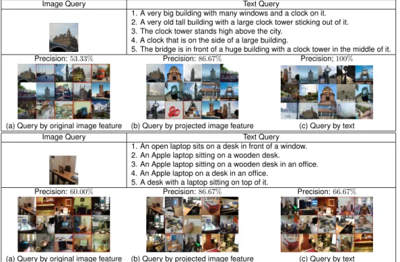
3.3 Sample retrieval results on the COCO dataset. The first row of each table presents the query image and text, and the second row shows the retrieved images by different query types. False positive results are bounded in red [P1]. 37 3.4 The adjacency relationship of the intrinsic and penalty graphs of the proposed MvNDA. The circular and rectangle dots indicate samples from different views. We illustrate the 2-nearest adjacencies (i.e. k1=k2= 2) of one sample in each class per view origin for clarity [P2]. . . 39

3.5 t-SNE Embedding of Latent Feature Representation: We visualize the embed-dings from different numbers of views using the proposed method [P2]. . . . 40

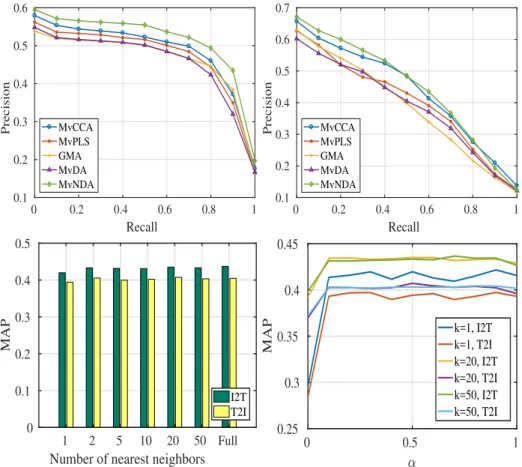
3.6 Clockwise from top left: The precision-recall curve by querying images for text annotations, the retrieval performance of matching text to images, the MAP scores with variousαunder different fixed numbers of nearest neighorsk, (herek=k1=k2), and the MAP scores with the differentknearest neighbors and a fixedα= 0.5. The legends in the figures in the first row indicate the method producing the PR curve, and we denote querying images for texts by “I2T”, and querying texts by images by “T2I” in the figure in the bottom row. k is the number of nearest neighbors [P2]. . . 41

3.7 Face-Sketch Recognition Rate for different probabilityp[P3]. . . 43 1

(11)

3.8 The correlation matrix between the measurements of Times Higher Education (THE) and Academic Ranking of World Universities (ARWU) rankings. The data is extracted and aligned based on the performance of the common universities in 2015 between the two ranking agencies. The reddish color indicates high correlation, while the matrix elements with low correlation are represented in bluish colors [P4]. . . 44 3.9 System diagram of the Deep Multi-view Discriminant Ranking (DMvDR). First,

the featuresX ={X1,X2, . . . ,XV}are extracted for data representations in

different views and fed through the individual sub-networkFv to obtain the

nonlinear representationZv of the vth view. The results are then passed

through two pipelines of networks. One line goes to the projectionW, which

maps allZv to the common subspace, and their concatenation is trained to

optimize the fused ranking loss with the fused sub-networkH. The other line

connectsZv to the sub-networkGv,∀v= 1, . . . , V for the optimization of the

vth ranking loss [P4]. . . 48 3.10 Rank correlation matrix for views 1-3 and the fused view [P4]. . . 52 3.11 A summary of multi-view deep learning methods. . . 53

(12)

List of Tables

3.1 The matricesPandQfor the proposed multi-view CCA, PLS and MvMDA [P1]. 32

3.2 RECOGNITION ACCURACY (%) on the AwA DATASET [P1]. . . 36 3.3 Recognition Rate (%) on the CUFSF Dataset [P3]. . . 43 3.4 Average Prediction Results (%) on 3 University Ranking Datasets in 2015 [P4]. 52

(13)

(14)

List of Symbols

1 An all-ones matrix

ci Class label of the samplexi

C Number of class

e A vector of ones

G A weighted graph

I Identity matrix

K Representation in the kernel space

LB Between-class Laplacian matrix

LW Within-class Laplacian matrix

P Inter-view covariance matrix

Q Intra-view covariance matrix

R A set of real numbers

W Data projection matrix

Wv Data projection matrix of thevth view

x A feature vector ofDdimensions

X A data matrix ofDdimensions byN samples

Xv Feature vectors of thevth view

d Dimensionality in the latent space

λ Eigenvectors

φ Nonlinear mapping function to the Hilbert space

Σ Covariance matrix

(15)

(16)

List of Abbreviations

CCA Canonical Correlation Analysis

GMA Gerneralized Multi-view Analysis

KMvPLS Kernel Multi-view Partial Least Square regressions

KapMvCCA Approximate Kernel Multi-view Canonical Correlation Analysis

KMvCCA Kernel Multi-view Canonical Correlation Analysis

KapMvPLS Approximate Kernel Multi-view Partial Least Square regressions

LMvCCA Linear Multi-view Canonical Correlation Analysis

LMvPLS Linear Multi-view Partial Least Square regressions

MvCCAE Multi-view Canonically Correlated Auto-Encoder

MvDA Multi-view Discriminant Analysis

MULDA Multi-view Uncorrelated Linear Discriminant Analysis

MvMDAE Multi-view Modularly Discriminant Auto-Encoder

MvNDA Multi-view Nonparametric Discriminant Analysis

RMSE Root Mean Square Error

(17)

(18)

List of Publications

The thesis is composed of a summary part and 4 publications listed below as appendices. The publications are referred in the thesis as [P1], [P2], etc.

[P1] G. Cao, A. Iosifidis, K. Chen and M. Gabbouj, “Generalized Multi-View Embedding for Visual Recognition and Cross-Modal Retrieval,” in IEEE Transactions on Cybernetics, vol. 48, no. 9, pp. 2542-2555, Sept. 2018. doi: 10.1109/TCYB.2017.2742705

[P2] G. Cao, A. Iosifidis and M. Gabbouj, “Multi-View Nonparametric Discriminant Analysis for Image Retrieval and Recognition,” in IEEE Signal Processing Letters, vol. 24, no. 10, pp. 1537-1541, Oct. 2017. doi: 10.1109/LSP.2017.2748392

[P3] G. Cao, M. A. Waris, A. Iosifidis and M. Gabbouj, “Multi-modal subspace learning with dropout regularization for cross-modal recognition and retrieval,” 2016 Sixth International Conference on Image Processing Theory, Tools and Applications (IPTA), Oulu, 2016, pp. 1-6. doi: 10.1109/IPTA.2016.7821032

[P4] G. Cao, A. Iosifidis, M. Gabbouj, V. Raghavan, R. Gottumukkala, Deep Multi-view Learning to Rank, submitted to IEEE Trans. on Knowledge and Data Engineering. arXiv:1801.10402

(19)

(20)

1 Introduction

1.1 Objective

The goal of the thesis is to analyze and learn data representations in different domains or feature types. In particular, the aim is to improve the performance of multi-view data analysis in numerous applications by exploiting the enriched information coming from various sources. Different groups of feature vectors are considered as views, and a view therefore includes feature vectors in a specific domain/modality, e.g. image, text or speech, or from a dedicated descriptor, e.g. color descriptor, texture descriptor, shape descriptor or audio descriptor. Cross-modal matching is also enabled on heterogeneous data, where direct matchings of data samples across feature spaces is infeasible. This is in contrast to applications like text-based image retrieval, which largely take advantage of ground truth textual labels surrounding the images. Although these applications are relatively successful under certain circumstances, the deficiency in developing the cross-modal learning capability limits them in fully understanding images.

Extracting informative data representations is a critical step in visual recognition and data mining tasks. It aims to bridge the semantic gap between the low-level feature represen-tations and high-level human comprehensible knowledge. This thesis introduces several techniques in learning multi-view data representations using subspace learning tech-niques, and formulates novel algorithms to enhance feature discriminability. The learned feature representation provides a discriminative input for the future tasks. Moreover, end-to-end solutions are formulated to strenghten the learning capabability by optimizing the entire system thoroughly. To this end, the performance of many challenging problems in visual recognition and data mining is improved.

1.2 Motivation

Our intuition is that, visual objects are described from various view points and/or modali-ties. The process of identifying an object can not only benefit from visual descriptions, but interactions with image captions and enriched attributes [2]. With a huge volume of data generated from sensor technologies, visual recognition and data mining problems urge

(21)

people to dive into multi-view and cross-domain learning [3, 4]. Meanwhile, the process of data acquisition across diverse domains or representations by using different types of feature extraction methods give rise to the heterogeneous property of data. Therefore, in order to analyze the heterogeneous data, multi-view and cross-modal learning algorithms are formulated to significantly improve the performance of machine learning [4, 3]. The research of multi-view data analysis is of great importance, and is able to improve the performance of numerous applications, which include but are not limited to

• Cross-modal Multimedia Retrieval. This application uses queries from one do-main (e.g. text) while seeking for similar contents from another dodo-main (e.g. image). Examples can be found in [5, 3, 6].

• Object Recognition.With high-level semantic information embedded in the recog-nition model, the object recogrecog-nition performance can be improved [7, 8].

• Face Photo-Sketch Recognition. The cross-modal matching between faces and sketches is made possible when their features are embedded in the shared subspace. Examples can be found in [9, 10].

• Multi-view Learning to Rank. The traditional ranking model evaluates the rele-vance between every pair of query and data by combining the features in an optimal way. In contrast, the relevance of the same pairs may differ from various ranking sources. A potential compositive ranking is provided as the solution to maximize the global agreement.

• Visual question answering. Two models are built to encode the visual and language views. Image and question embeddings are combined to obtain a single model, so that the visual question answering can be achieved [11].

1.3 Thesis Outline

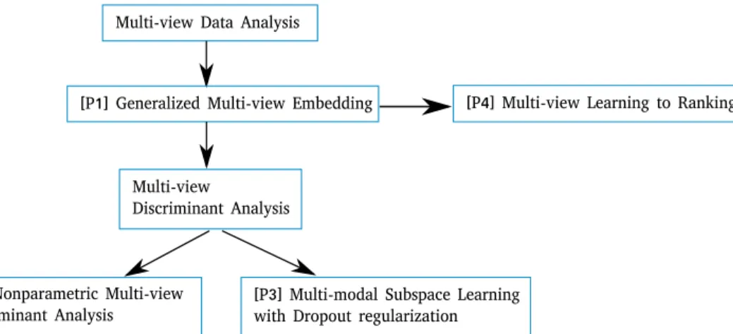
The rest of the thesis is organized as follows. Chapter 2 reviews the literature of subspace learning, regularization and in particularly multi-view learning. The thesis contribution is presented in details in Chapter 3. A unified formulation to generalize the multi-view subspace learning methods is introduced. It is then extended to nonlinear mappings using kernels and neural networks. A new regularization scheme form linear multi-view subspace learning is described to prevent overfitting. A nonparametric multi-view learning technique is also introduced, which enables multiple projection directions, by relaxing the Gaussian distribution assumption of related methods. In the end, a composite ranking method from multiple sources is proposed to enhance the joint ranking and minimize the view-specific ranking loss. A schematic diagram illustrating the relation between methods in the thesis is shown in Figure 1.1.

(22)

1.4. Contributions and Publications 13 Multi-view Data Analysis

[P1] Generalized Multi-view Embedding

[P2] Nonparametric Multi-view Discriminant Analysis

Multi-view Discriminant Analysis

[P3] Multi-modal Subspace Learning with Dropout regularization

[P4] Multi-view Learning to Ranking

Figure 1.1:The schematic view of the thesis outline.

1.4 Contributions and Publications

The major contribution of this thesis is the proposal of a unified framework of multi-view data mapping, which is described in [P1]. A nonparametric extension is introduced in [P2], and further extension with Dropout-like regularization can be found in [P3]. Moreover, a multi-view learning to rank method, as an importance application of multi-view data analysis, is developed and described in [P4].

In [P1], an unified solution for subspace learning methods is proposed using the Rayleigh quotient, which is extensible for multiple views, supervised learning, and nonlinear embeddings. The proposed framework is generalized to numerous statistical learning methods including Canonical Correlation Analysis, Partial Least Square regression and Linear Discriminant Analysis with graphs in specific forms. It is also extented to nonlinear mappings using kernel and neural network-based methods. A simple yet effective Multi-view Modular Discriminant Analysis is proposed by introducing the Multi-view difference. The proposed multi-view embedding methods have shown superior performance in visual object recongition and cross-modal multimedia retrieval. The candidate is the first author of this publication and is responsible for developing most of the methods, performing all experiments and writing the manuscript.

In [P2], a novel multi-view nonparametric discriminant analysis method is proposed and achieves superior performance in cross-modal image retrieval and zero-shot recognition. The class boundary structure and view discrepancy is exploited to formulate an opti-mization criterion which is automatically adjusted to the multi-view class structures. The advantage of the new method is that it enables multiple projection directions, by relaxing the Gaussian distribution assumption of related methods. A better class discrimination is obtained using the new graph formulation leading to an improved performance. The candidate is the first author of this publication and is responsible for developing the whole methods, performing all experiments and writing the manuscript.

(23)

In [P3], inspired by the regularization for neural networks, a novel regularizer is introduced to artificially remove the effect of certain amount of feature bins using the probabilistic approach to prevent linear multi-view subspace learning from overfitting. A joint dropout-regularized multi-modal subspace learning algorithm is formulated which integrates within-class similarities and between-within-class separabilties to achieve good within-class separation. The objective function can be solved efficiently, and the method demontrates its effectiveness in face-sketch recognition and cross-modal retrieval problems. The candidate is the first author of this publication and is responsible for developing the whole methods, performing all experiments and writing the manuscript.

In [P4], a multi-view learning to rank is developed, which is one of the few methods in data mining. A composite ranking method is introduced to keep a close correlation with the individual rankings. Multi-objective solutions to ranking is devised by capturing the information of the feature mapping from both within each view as well as across views using autoencoder-like networks. Moreover, we introduce an end-to-end solution to enhance the joint ranking with minimum view-specific ranking loss, so that the maximum global view agreement is achieved in a single optimization process. Superior ranking results are achieved on university ranking, multi-view lingual text ranking and image data ranking problems. The candidate is the first author of this publication and is responsible for developing the whole methods, performing all experiments and writing the manuscript.

(24)

2 Related Work

In this chapter, we firstly review the subspace learning algorithms. Then, several impor-tant regularization methods are reviewed. Relevent methods in multi-view learning are elaborated. Finally, some applications of interest are provided.

2.1 Subspace Learning

Subspace learning is an important data analysis approach which is used to extract salient features from data. The main idea is to project the high-dimensional data into the low-dimensional space by fitting certain criteria, so that the relevant information to the subsequent processing is maintained [12, 13]. This type of approaches can be classified into three categories, based on the availability of class labels: unsupervised methods, supervised methods and semi-supervised methods. Unsupervised methods learn the underlying data patterns by using the similarities between samples. Traditional methods like principal component analysis (PCA) belong to this category. Supervised methods are effective in extracting discriminative features from the labeled data, and thus leading to good results in classification. Linear discriminant analysis (LDA) as the most representative supervised method, shows superior results in face recognition compared to PCA [14]. Semi-supervised methods make use of both labeled and unlabeled data, e.g. semi-supervised discriminant analysis (SDA) extends the objective function of LDA by using a graph-based regularization term. Many subspace learning methods can be described as specific cases of the graph embedding framework [15]. We describe these techniques in details in following sections.

2.1.1 Graph Embedding

Graph embedding has been considered as a general framework for dimensionality reduction [15, 16]. The basic idea is to find a mapping functionF:X∈RD×N _→_Y_∈

Rd×N _{to map the data from the original high-dimensional space to a low-dimensional}

space, whereD > dis the dimensionality of the feature space andN is the number of samples. The functionFcan be linear or nonlinear, implicit or explicit, depending on the method used to define the data projection. The method assumes that we can develop

(25)

a weighted graphG ={X,V}with similarity matrixV∈ RN×N _{over the training data}

X= [x1,· · ·,xN]∈RD×N. A graph Laplacian matrixL=D−Vcan then be defined,

where

D[i, i] =X

j

Vij, andD[i, j] = 0for∀i6=j. (2.1)

We also define a penalty graphGp ₌_{_X_,_Vp_}_{formed by the same vertices}_X_{but using}

a different similarity weight matrixVp_{. The data is projected to a latent space, where the}

similarity charateristics ofVpare suppressed. Considering the sample-wise projection to y= [y1, y2,· · ·, yN]∈Rd, the graph-preserving objective is

W∗= arg min Tr(y Cy>₎₌_q X i6=j kyi−yjk2Vij = arg min Tr(y Cy>₎₌_q y Ly>, (2.2)

whereqis a constant andCis a matrix used to constrain the minimization of the objective function.Cis also a diagonal matrix for scale optimization, and can also be the Laplacian matix of a penalty graphGp_{. In the latter case,}_C₌_Lp₌_Dp₋_Vp_{. Similar to (2.1),}_Dp

is the diagnal matrix. The graph-preserving objective is the criterion of graph embedding for all vertices. While the graph vertices in direct graph embeddings only presents the training data, it can be extended to new test data in the original feature space.

The mappingF:X→Ydefined by 2.2 can take three forms:

Linear:We consider linear projections of the original dataxi ∈RDto a low-dimensional

feature spaceRd_{, d < D}_{, which is expressed as}_Y₌_W>_X_{, where}_W_∈_RD×d _{is the}

data projection matrix. The objective function in (2.2) can be expressed as W∗= arg min Tr(W>_XCX>_W₎₌_q X i6=j kW>xi−W>xjk2Vij = arg min Tr(W>_XCX>_W₎₌_q W>XLX>W, (2.3)

Kernel-based: The idea behind kernel methods is to map the data from the original feature spaceRD _{to a higher dimensional Hilbert space}_F_{. Let us define}_φ₍_·₎_{as the}

nonlinear function mappingxi∈RDtoF, andΦ= [φ(x1), . . . ,φ(xN)]as the data matrix

inF. The kernel trick [17] is exploited in order to implicitly map the data to arbitrary space F, and the kernel matrixK =Φ>Φcontains the inner products between the training samples in the Hilbert space, which can also be written as

[K]ij=κ(xi,xj)] =φ(xi)>φ(xj), (2.4)

whereκ(·,·)is the so-called kernel function. The centered Gram matrix isK¯ = K−

1 N1 K− 1 NK 1 >₊ 1 N21K 1, where1∈R

N×N _{is an all-ones matrix. In order to find the}

optimal projection, we can expressWof each view as a linear combination of the training samples in the kernel space based on the Representer Theorem [18, 19]. The data

projecttion matrix can be expressed by using a new weight matrixAas

(26)

2.1. Subspace Learning 17 The feature mapping in kernel methods can be derived as

Y=W>Φ=A>Φ>Φ=A>K. (2.6)

The objective function in (2.2) is written as A∗= arg min Tr(A>_KCKA₎₌_q X i6=j kA>ki−A>kjk2Vij = arg min Tr(A>_KCKA₎₌_q A>K L KA (2.7)

Neural networks-based: The data mappnigFcan take the form of a neural network with

M layers, whereθj contains the weight parameters in thejth layer,j = 1, . . . , M. The

network weightsΘ = [θ1, . . . ,θM]are learned by applying stochastic gradient descent

(SGD), andF(·; Θ)is a nonlinear mapping function which mapsXto the representation of the last hidden layerZof the network, i.e.

Z=F(X; Θ). (2.8)

Θis the weight matrix trained by applying backpropagation in the network. The objective

function in (2.2) for feature mapping using the hierarchical representation obtained using the neural network is expressed as

W∗= arg min Tr(W>_ZCZW₎₌_q W>ZLZ>W (2.9) = arg min Tr(W>_W₎₌_q W>ZLZ>W W>_ZCZ>_W, (2.10)

whereCis the Laplacian matrix of the penalty graphGp_{. The optimization problems in}

(2.3), (2.7) and (2.10) can be solved as a generalized eigenvalue problem in the following

Lv=λC v, (2.11)

whereλis the set of eigenvalues andvis the set of eigenvectors.

2.1.2 Dimensionality Reduction

2.1.2.1 Unsupervised Methods

PCA is the classical method for dimensionality reduction by maximizing the variance of data in the projection space. PCA makes three general assumptions:

1. Linearity: PCA is limited to re-expressing the data as alinear combinationof its basis vectors.

2. The data with large variances contains important structure. Specifically, by as-suming the data has a high signal to noise ratio, principal components with larger associated variances represent interesting information.

(27)

3. The principal components are orthogonal. It allows an intuitive simplification which makes PCA solvable with linear algebra decomposition techniques.

The detailed process is summarized as follows. GivenX ∈ RD×N_{, where}_D _{is the}

number of dimensions andN is the number of samples, we firstly center the data

¯

X=X− 1

NX. Then, the SVD is calculated to the half of the input data which is

1

√ NX¯

>_,

or the eigenvectors of the covariance (ΣX= _N1XX>).Wis a subset of the eigenvectors

corresponding to the leading eigenvalues. Finally, we can projectXto the new spaceY with a reduced dimensionality asY=W>X.

PCA finds and removes the projection directions with minimal variance, which can be expressed in graph embedding as

W∗= arg max W>_W₌₁

W>ΣW, (2.12)

whereΣ= _N1X(I− 1

Nee

>₎_X> _{is the covariance matrix,}_e_{is an N-dimensional vector of}

ones andIis an identity matrix.

Partial least squares (PLS) regression [20] also finds a linear combination of input basis vectors for regression. It peroforms the eigenanalysis of a variance matrix between inputsXandY. As in the case of PCA, the scaling of the variables has a impact on the solutions of the PLS. When expressing the PLS as a graph embedding , the variance

betweenX andY, i.e.

Σ=   0 ΣXY ΣXY 0   (2.13) is used in (2.12). 2.1.2.2 Supervised Methods

Linear Discriminant Analysis (LDA) [21] finds a projection by maximizing the ratio of the between-class scatter to the within-class scatter. Let us define byµcthe mean vector of

thec’th class, formed byNcsamples, andµthe global mean. Then, LDA optimizes the

following criterion: J = arg max W>_W₌_I Tr(W>P W) Tr(W>_{Q W}₎ = arg max W>_W₌_I Tr(W>XCX>W) Tr(W>_{XL X}>_W₎, (2.14) where P= C X c=1 Nc(µc−µ)(µc−µ)>=X C X c=1 1 Nc ecec>− 1 Ne e >_X>_, _(2.15) Q= N X i=1 (xi−µc)(xi−µc)>=X I− C X c=1 1 Nc ecec> X>. (2.16)

(28)

2.2. Regularization 19 Nonlinear extensions with kernels include KDA [22] and KRDA [23].

Locality Preserving Projections (LPP) [24] seeks theknearest neighbors of the samplexi,

among the samples having the same class label asxi. It preserves the local information,

and obtains a latent space which contains the salient manifold structure. The data projection matrixWis obtained using the same generalized optimization form as (2.14), while its graph Laplacian matrixCof the penalty graph is formulated by integrating the discriminative information as follows

C=    e− kxi−xjk2 2σ2 _, if_x i∈Nk(xj)orxj∈Nk(xi); 0. otherwise. (2.17)

2.2 Regularization

A model is trained involving allDdimensions, but the estimated coefficients are shrunken towards zero relative to the least squares estimates. The regularization method also known as shrinkage has the effect of reducing variance and can perform variable selection [25]. It has been largely applied to tackle model overfitting. We discuss several recent techniques for regularization.

2.2.1

`

p

-norm Regularization

An additional regularization term is added to the objective function to reduce the model complexity. Suppose we have a loss functionL(X,y|θ), the regularized objective then is

ˆ

L(X,y|θ) =L(X,y|θ) +αR(θ), (2.18)

whereR(θ)is the regularization term, andαis a control parameter.

The general form of`p-norm based regularization isR(θ) =Pjkθjkpp. Whenp≤1, the

objective is a convex optimization problem. In particular, the`2-norm regularization is commonly used which is known as weight decay. Whenp≤1, the resulting regularization

exploits the sparsity of the objective function with a non-convex optimization.

2.2.2 Dropout and DropConnect

Dropout [26, 27] has been originally proposed as a regularization strategy for neural networks training. It prunes the neurons in the network to effectively regularize the model in an online fashion. It can be also considered analogously as a bagging ensembles of many large neural networks, which learns the network output weights. The outputs of the synthetic hidden layer by dropout is written as

(29)

where◦denotes the Hadamard product of two vectors andmi,t ∈Rnlis a binary mask

vector with each element equal to1with probabilitypand equal to0with(1−p), and

nlthe number of neurons in thelth layer. We denoteias the number of samples, and

tis the epoch of network training. The binary maskmi,tis selected independently for

each sample from a Bernoulli distirbution and changes over the training iterations, and therefore, the trained model is a bagged ensemble of neural networks. The difference with a traditional bagging method is that the neural networks using bagging share parameters from the original (full) neural network.

Besides dropout regularization, we can also set the elements of output weight matrixW

to zero, which effectively drops the connections between neurons. The synthetic hidden layer outputs by DropConnect are

z=ψi,t(M◦W>)x), t= 1,· · ·, N, t= 1,· · ·, T, (2.20)

where Mi,t ∈ Rnl×n(l−1) is a binary mask matrix with its elements equal to 1 with

probabilitypand (1−p)otherwise. Both Dropout and DropConnect use the masked

versions of weight for nerual network training.

2.3 Multi-view learning

2.3.1 Overview

In general, a view is referred to as a group of features extracted from a domain or modality. The modern process of data acquisition across various sensory modalities gives rise to the heterogeneous property of data. Multiple features can be generated in diverse domains or using different descriptors to represent the same data sample. Multi-view learning is the set of methods which leverage the information of heterogeneous data [4]. The goal of multi-view learning is therefore to integrate multiple views to make effective decisions.

There is a considerable difference between conventional machine learning algorithms and multi-view learning. The former takes a single-view input or a concatenation of multiple views, trains a model and generates an output of single view. By contrast, its multi-view counterpart joinly learns a model by optimizing a function from the multiple views, and make predictions using the enriched information. Methods to exploit the sensory redundancies, which contains both common and complementary information, can be classified into three groups, including subspace learning, co-training and multiple kernel learning.

We can categorize the methods of multi-view learning based on the tasks that we want to achieve [28]: representation, translation, alignment, fusion and co-learning. Representation learning is a task to extract a feature representation by learning a mapping

(30)

2.3. Multi-view learning 21 function from the original data. Subspace learning providing a compact representation belongs to this category. Translation considers feature mapping from one modality to another, so that a cross-view learning can be achieved. Alignment is to find the matches in elements between modalities. Fusion aims to integrate the multi-view information for making predictions. Multiple kernel learning belongs to this category. Finally, co-learning considers transferring knowledge across modaltiies. Co-training and zero-shot learning are examples of this type of methods. We will elborated the important multi-view learning methods in the following sections.

2.3.2 Multi-view Subspace Learning

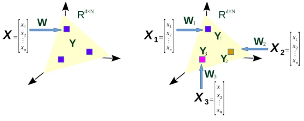
The challenge in multi-view learning is that there exists a large discrepency between views. Mapping each of the views to their own subspace does not provide good matches between projected features. Multi-view subspace learning mitigates the problem by projecting them into a common latent space by optimizing a joint criterion. We present this idea in Figure 2.1.

R

d×N

X

=

[

x1 x2 ⋮ xn

]

W

Y

R

d×N

X

1=

[

x1 x2 ⋮ xn

]

W

Y

X

2=

[

x1 x2 ⋮ xn

]

1

W

2

X

₃=

[

x1 x2 ⋮ xn

]

W

3 1

Y

3

Y

2

Single-view subspace learning

Multi-view subspace learning

Figure 2.1:Single-view subspace learning projects one input to a latent space, while multi-view

subspace learning leverages a common space from multiple inputs.

2.3.3 Unsupervised Multi-view Subspace Learning Methods

2.3.3.1 Linear CCA

Canonical Correlation Analysis (CCA) [29, 30] is a conventional statistical technique

which finds the maximum correlation between two sets of data samplesX1∈_RD1×N

(31)

W2are determined by optimizing: J = arg max W1,W2 corr(W>₁X1,W>2X2) (2.21) = arg max W1,W2 W>₁Σ12W2 p W>₁Σ11W1·pW>₂Σ22W2, (2.22) where Σ= " Σ11 Σ12 Σ21 Σ22 # = 1 N "_¯ X1X¯>1 X1¯ X¯>2 ¯ X2X¯>1 X¯2X¯>2 # (2.23) 2.3.3.2 Kernel CCA

Kernel CCA finds the maximum correlation between two views after mapping them to the kernel space [31]. It is expressed mathematically as

J = arg max W1,W2

corr(W>₁Φ1,W>₂Φ2) (2.24)

Using the kernel trick [17] and the Representer Theorem in (2.5), the objective function for the kernel CCA becomes

J = arg max Tr(A> 1CA2)=p A>1K1K2A2 p A>₁K1K1A1·pA>₂K2K2A2. (2.25) 2.3.3.3 Deep CCA

Deep CCA maximizes the correlation between a pair of views by learning nonlinear representations from the input data through multiple stacked layers of neurons [32, 33]. A linear CCA layer is added on top of both networks, and the inputs to the CCA layer depend on the network outputsZ1and Z2. Similar to the nonlinear case in (2.25), a

modified objective function min

W1,W2

−1

N Tr W1

>_Z1_Z>_W2

is optimized, whereW1,W2

are the projection matrices in the CCA layer, and the correlated outputs areY1=W>₁Z1 and Y2 = W>2Z2. A modified SGD method is developed with respect to the inputs

Z1 andZ2to the linear layer, which are also the outputs from the two networks. The

objective function is expressed asTr W>₁Z1 Z>2W2

= Tr(T>T)12, which describes the correlation as the sum of the topdsingular vectors ofT=Σ₁₁−1/2Σ12Σ−₂₂1/2whose definition can be found in [34]. The projection matrices are obtained from the singular value decomposition ofT, asT=W1DW>2. The gradient is then computed as

∂(Tr(T>T)12) ∂Z1 = 2∆11Z1+ ∆12Z2, (2.26) where ∆12=Σ −1/2 11 W1W>2Σ −1/2 22 (2.27) ∆11=− 1 2Σ −1/2 11 W1DW>1Σ −1/2 11 . (2.28)

(32)

2.3. Multi-view learning 23

2.3.4 Supervised Multi-view Subspace Learning Methods

2.3.4.1 Multi-view Discriminant Analysis (MvDA)

MvDA [35] is the multi-view verison of LDA which maximizes the ratio of the traces of the between-class scatter matrix to that of the within-class scatter matrix. Its objective function is J = arg max W Tr(SB) Tr(SW) , (2.29)

where the between-class scatter matrix is SB = V X i=1 V X j=1 W>_i Xi C X c=1 1 Nc ecec>− 1 Ne e >_X> jWj, (2.30)

and the within-class scatter matrix is SW = V X i=1 V X j=1 W>_i Xi I− C X c=1 1 Nc ecec> X>_jWj. (2.31)

Wcontains the eigenvectors of the matrixS=SW−1SB corresponding to the leadingd

eigenvaluesλi.

2.3.5 Multi-view Uncorrelated Discriminant Analysis (MvUDA)

Multi-view Uncorrelated Discriminant Analysis is an extension of MvDA inspired by the uncorrelated discriminant transform in [36]. We consider the method in 2 views. Following the same form of objective function as MvDA in (2.29), it multiplies a uncorrelated term with between-class scatter matrix, and the solution is

" P1 0 0 P2 # " Sb1 γΣ12 γΣ12 Sb2 # " W1 W2 # =λ " Sw1 012 0 σSw2 # " W1 W2 # , (2.32)

whereP1andP2uncorrelate the between-class scatters, and are expressed by

P1=I−Sw1W > 1(W1Sw1W > 1) −1_W1_, P2=I−Sw2W > 2(W2Sw2W > 2) −1_W2_.

γandσare scaling parameters.

2.3.6 Semi-supervised Learning

Co-training method [37] is a semi-supervised learning method which maximizes the mutual agreement on a pair of distinct views of the unlabeled data. It provides a superior classification performance under the following assumptions.

• The training samples contain two sufficient sets of features (X1,X2), while each sample has two corresponding views (x= [x1,x2]).

(33)

• The two views are independent given the class label, i.e.

P(X1|X2,y) =P(X1|y), (2.33)

P(X2|X1,y) =P(X2|y). • The two views are consistent:

∃f1, f2:fco-trained(X) =f1(X1) =f2(X2). (2.34) The method has been well recognized, and many efforts have been made beyond its original usage in text mining for search engine. Expectation-maximization (EM) was successfully applied to classify new samples between classifiers using a probabilistic approach [38]. Multi-view spectral clustering is enabled by introducing a co-regularization to the clustering in [39]. Bayesian view of co-training is developed in [40]. Co-training is also extended for learning to rank in [41].

2.4 Applications

Multi-view subspace learning can be used in numerous application domains. In the following, we briefly describe the major applications used in the thesis to evaluated the performance of the proposed methods.

2.4.1 Cross-modal Multimedia Retrieval

Traditional multimedia retrieval applications consider unimodal scenarios. Typical ex-amples in this case include text search by matching strings or related topics, and content-based image retrieval [42, 43]. In contrast to unimodal solutions, multimodal retrieval systems have been developed mainly about image retrieval using text queries [44, 45, 46, 47]. Large multimedia repositories such as TRECVID [48] and ImageCLEF [49] have been collected to study and evaluate the retrieval over multiple modalities. However, these methods are still based on the unimodal approach, e.g. people use text queries to match the tags surrounding the images to search for the relevant images. There is an increasing amount of efforts in cross-modal retrieval. Traditionally, the text annotations of images can be scarsely found. Thanks to sensor technologies and popularity of internet services, there is an explosion of multimedia content avaiable online, and these data are richly annotated with full descriptions. Manifold learning has been successfully applied from a matrix of distances between multimodal objects [50, 51, 52]. The multimodal distances are formulated as a function of distances between each pair of modalities, which allows mis-matched pairs. However, it limits the queries to the training set which is used to learn the manifold. Recently, a new cross-modal retrieval method [3] is developed by exploiting the correlation between modalities and mapping the feature

(34)

2.4. Applications 25 in the latent space towards to the semantic labels. Superior retrieval performance has demonstrated the effective combination of correlation and semantic matching.

A very big building with many windows and a clock on it. A very old tall building with a large clock tower sticking out of it. The clock tower stands high above the city. A clock that is on the side of a large building. The bridge is in front of a huge building with a clock tower in the middle of it. An open laptop sits on a desk in front of a window.

An Apple laptop sitting on a wooden desk. An Apple laptop sitting on a wooden desk in an office. An Apple laptop on a desk in an office. A desk with a laptop sitting on top of it.

Text Space

Image Space

Latent Space _{Semantic Space}

Semantic Concept1: Car Semantic Concept2: Building Semantic Concept3: Bedroom

Figure 2.2:An illustration of cross-modal image retrieval.

2.4.2 Zero-shot Object Recognition

Zero-shot object recogntion [53] is an emerging topic which aims to recognize objects of unseen classes. It is inpired from the real-world scenario of human categorizing new objects or generalizing novel concepts. The approach has a strong connection with learning to learn [54], and lifelong learning [55]. The main idea is to establish a relation from the objects in the source domain (seen classes) to the target domain (unseen classes) using a universal semantic representation. There are several ways to generate the semantic representation or attributes, which includes user-defined attributes [56, 57], relative attributes [58, 59, 7], and data-driven attributes [60, 61]. The transferrable knowledge enables the object recognition of unseen classes. Visual features are mapped to the latent space of semantic representations. The unlabeled target class is projected in the same space. One major problem of zero-shot recognition is that data distribution of the source classes and target classes is different, and therefore a domain shift is found when projecting both data from both domains to the same latent space. The problem is allieviated by introducing a multi-view semantic latent space which fuses data from multiple modalities [7].

2.4.3 Face-sketch Recognition

Face-sketch recognition is an important application enabling searches of potential sus-pects in a mugshot database created by law enforcement. The main idea is to shortlist the photos in the database which may match to the face of the suspect. Usually, sketches are

(35)

drawn based on the description by the eyewitness, and the most distinctive facial features are presented on the sketches. However, sketching a face involves many psychological factors, which may result in misleading face recognition. Some examplar images from the face-sketch database are shown in Figure 2.3.

Figure 2.3:Examplary face-sketch image pairs in the CUFSF dataset [1].

Subspace learning has been successfully applied in the face-sketch recognition [62, 63]. Linear mappings between faces and sketches using PCA was introduced in [62]. Kernel-based LDA was also applied as the nonlinear mappings Kernel-based on image patches [63]. Another extension in [64] is to perform random feature sampling and calculate kernel prototype similarities before applying LDA. There are many efforts which project both modalities into a common subspace. For example, coupled discriminant analysis is introduced in [65] to learn from faces and sketches in a common latent space. Directly learning the image filters from the raw faces and sketches simultaneously also shows its effectiveness in heterogeneous face recognition [66]. Image patches are represented using Markov random fields to incorporate the spatial information in patch neighborhoods [67]. A novel similarity metric is also proposed to calculate the distance between faces and sketches.

2.4.4 Learning to Rank

Ranking problems can be found in numerous applications, for example ratings of food or movies, image retrieval and ranking [68, 69], image quality ratings [70], online advertising [71], and text summarization [41]. In general, there is a series of data pre-processing and indexing to generate the pairs of queries and samples for matching. The ranker, which is the key comoponent, provides a relevance score between each pair of query and sample. The score can be calculated based on some heuristic measure or learning approach. Learning to rank aims to optimize the combination of data representation for ranking

problems [72]. We present its framework in Figure 2.4. Suppose we haveN training

samples, which consists ofqtr,Xtrandytr.Xtr= [x1,x2,· · · ,xN]>is the feature

vec-tors of the training data, wherexn∈RDrepresents itsnth sample.qtr = [q1, q2,· · ·, qn]

is the corresponding query andytr _{= [}_y

(36)

2.4. Applications 27 ranking modelhis learned over the training data, and makes predictions over the test dataqte_,_Xte_{. We predict its relevance}_h₍_qte_,_Xte₎_{using the trained model}_h_.

Training Data

Ranking Model

Test Data

Learn

Predict

Prediction

Figure 2.4:The framework of Learning to Rank.

Solutions to this problem can be decomposed into several key components, including the input feature, the output vector and the scoring function. The framework is developed by training the scoring function from the input feature to the output ranking list, and then, scoring the ranking of new data. Traditional methods also include engineering the feature using the PageRank model [73], for example, to optimally combine them for obtaining the output. Later, research was focused on discriminatively training the scoring function to improve the ranking outputs. The ranking methods can be classified in three categories for the scoring function: the pointwise approach, the pairwise apporach, and the listwise approach.

The pairwise approach is considered in the thesis and therefore reviewed thoroughly as follows. A neural network which learns a preference function was developed in [74] to directly evaluated the pairwise order between pairs of documents. RankNet [75] learns a neural network to optimize the pairwise ranking loss using a cross-entropy loss. The pairwise methods generally assume the scoring function to be linear [76], so the ranking data can be easily transformed to orders in pairs. The transformed data enables a binary classification for ranking, and therefore numerous classifiers have been applied. Adaboost algorithm [77] was successfully applied by iteratively reducing the classfication errors between each pair of documents, which can subsequently improve the overall output. Ranking SVM [78] adopted SVM to perform pairwise classification. GBRank used Gradient Boost Trees [79] in ranking documents. Semi-supervised multi-view ranking (SmVR) [41] is a co-training extension to ranking. Recently, there is an increasing amount of research in optimizing the evaluation metric for ranking. Examples include AdaRank [80], which optimizes the ranking errors iteratively, and LambdaRank [81]. While certain success has been obtained by the aforementioned methods, ranking multi-facet documents is important yet few can be found in literature [82, 83, 84].

(37)

2.4.4.1 Bipartite Ranking

The pairwise transform is critical for the success in ranking and therefore described explicitly in this section. The training data is defined in query-sample pairs{(xq_i,yq_i)},

whereq∈ {1,2, . . . , Q},xq_i ∈Rdis thed-dimensional feature vector for the pair of query q, thei-th sample,yq_i ∈ {0,1}is the relevance score, and the number of query-specific

samples isNq. The pairwise transformation to generate the query-sample pairs, so that

only the samples that belong to the same query are evaluated [76]. The relevance between each pair is defined as

pq_i(φ) = 1

1 + exp(φ(xi)−φ(xq))

,

whereφ: x→ _Ris the linear scoring function asφ(x) = a>x, which maps the input feature vectors to the scores. Due to its linearity, we can transform the feature vectors and relevance score into (x_k0,y0_k) = (xq−xi,yqi). In case of the ordered list (r) as the raw

input, each data samplexipaired with its queryxqis investigated, and their raw orders

(ri,rq) are transformed asy q

i = 1,ifri<rq; y q

i = 0, else ifri>rq. In pairwise ranking,

the relevanceyq_i = 1, if the query and sample are relevant, andyq_i = 0, otherwise.

The feature difference(x_k0,y0_k)becomes the new feature vector as the input data for

nonlinear transforms and subspace learning. Therefore, the probability can be rewritten as pk(φ) = 1 1 + exp(−φ(x0_k))= 1 1 + exp(−a>_x0 k) . (2.35)

The ranking loss is formulated as the cross entropy loss such that, `Rank= arg min

Q X q=1 Nq X i=1 yq_ilogpq_i) + (1−yq_i) logpq_i) = arg min K X k=1 y0_klogpk) + (1−y0k) logpk) , (2.36)

which is proved in [75] that it is an upper bound of the pairwise 0-1 loss function and optimized using gradient descent. The logistic regression or softmax function in neural networks can be used to learn the scoring function.

(38)

3 Contributions

This chapter describes the novel contributions of the thesis. We will begin with the generalized multi-view embedding method, which is the major contribution of the the-sis. Its extention to a multi-view non-parametric method exploiting the class boundary structure and discrepancy in views is subsquently described. Additionally, the dropout regularization is introduced to the linear multi-view analysis. Finally, we will present composite ranking methods for ranking problems which enhance the joint ranking with minimum loss from each ranking source.

3.1 Generalized Multi-view Embedding

We propose a unified solution for multi-view subspace learning which generalizes several statistical, supervised and nonlinear embeddings. Here, we solve the generalized optimization problem

J = arg max W

Tr(W>PW)

Tr(W>_QW₎ (3.1)

wherePandQare the matrices describing properties of the data to be maximized and

minimized, respectively, through embedding. We consider it as the uniform objective function, reaching out to a large number of subspace learning methods. A generalized eigenvalue problem is addressed when maximizing the criterion:

PW=ρQW, (3.2)

and the solution is given in the following form:

W=      W1 ... WV      andρ= d X i=1 λi. (3.3)

W, ρare the generalized eigenvector and the sum of the topdgeneralized eigenvalues λi, respectively. Wcontains the projection matrices of all views, andρis the value of

Rayleigh quotient in (3.1). The nonlinear multi-view embeddings can be achieved by 29

(39)

using kernel-based mappings, or (deep) neural networks optimized by SGD. In the case of linear projections, i.e. whenY=W>X, we derive the objective function based on [15, 85] as follows

J = arg max W>_W₌_I

Tr(W>XL0X>W)

Tr(W>_XLX>_W₎. (3.4)

In the kernel case, we have

J = arg max A>_KA₌_I

Tr(A>K L0KA)

Tr(A>_{K L KA}₎. (3.5)

In the above, we defineLas the total graph Laplacian matrix. Similarly, the penalty graph Laplacian matrix is denoted byL0.

In the case of the nonlinear embedding using neural networks, we apply a joint linear embedding layer on top of the neural networksFv, wherev= 1,· · · , V. The scheme is

presented in Figure 3.1. We train V sub-networks whose outputs are projected to a com-mon subspace using a linear projectionWv. We denoteF(X) = [F1(X1),· · · ,FV(XV)]>

as the concatenation of the neural network outputs. By doing so, the objective has the same form as in the linear case. By following the direction of the gradient for training the neural network, we optimize the Rayleigh quotient criterion with respect to the nonlinear feature representation from each view in the last hidden layer of the networks. The entire network is trained in a single optimization process.

Neural Network Neural Network Neural Network

Figure 3.1:Schematic presentation of Multi-view (Deep) Embedding Networks.

We illustrate the proposed framework graphically in Figure 3.2. Suppose we initially extract three types of low-level features from images, texts, and intermediate representa-tions. The multimodal features are projected using either linear or nonlinear projections to the common latent space. The projected features characterize the properties of the intra-view compactness and inter-view separability based on the Rayleigh quotient criterion.

3.1.1 Scaling Up the Inter-view and Intra-view Covariance Matrices

Numerous statisitical subspace learning methods can be generalized in the form of (3.1) by scaling up the inter-view and intra-view covariance matrices. Multi-view CCA (MvCCA) presented in [P1] maximizes the correlation between all pairs of views. Its objective can be rephrased as maximizing the inter-view covariance while minimizing the intra-view

(40)

3.1. Generalized Multi-view Embedding 31 Image Space 1 Image Space 2 RD ×N RD ×N2 Text Space R Attribute Space R Φ

Linear or Non-Linear Subspace Learning

The common space by maximizing Rayleigh quotient criterion (a) Linear methods

(b) Kernel methods

(c) Neural network methods

R Feature Extraction 1 D ×N3 D ×N4 d×N

Figure 3.2:Overview of the generalized multi-view embedding: Features from different modalities

are extracted and either linearly or nonlinearly mapped into the common subspace by maximizing the Rayleigh quotient criterion [P1].

covariance in the latent space. Therefore, we consider inter-view covariance matrices

between different view representations inPand the covariance matrices of each view

in Q. Multi-view PLS (MvPLS) maximizes the inter-view covariance directly, and its

difference with MvCCA is the intra-view minimization. Taking the class discrimination into consideration, the proposed multi-view modular discriminant analysis (MvMDA) extends to separate the data of different classes between views while making the intra-class data

compact. We present the structure ofPandQfor each method in Table 3.1.

3.1.2 Linear Subspace Learning

When the subspace projection is linear, we can obtain the latent feature vectors from each view as

Yv =W>vXv, (3.6)

which corresponds to the case on the top of Figure 3.2 using the linear feature mappings. Its projection matrix is obtained by directly solving the generalized eigenvalue problem in (3.2). Multi-view CCA minimizes the diagnal matrix and maximizes the off-diagonal matrix of the total covariance matrix shown in Table 3.1. we derive its projection matrix

(41)

Table 3.1:The matricesPandQfor the proposed multi-view CCA, PLS and MvMDA [P1]. P Q MvCCA       0 Σ12 · · · Σ1V Σ21 0 · · · Σ2V ... ... ... ... ΣV1 ΣV2 · · · 0             Σ11 0 · · · 0 0 Σ22 · · · 0 ... ... ... ... 0 0 · · · ΣV V       MvPLS       0 Σ12 · · · Σ1V Σ21 0 · · · Σ2V ... ... ... ... ΣV1 ΣV2 · · · 0             I 0 · · · 0 0 I · · · 0 ... ... ... ... 0 0 · · · I       MvMDA       P11 P12 · · · P1V P21 P22 · · · P21 ... ... ... ... PV1 PV2 · · · PV V             Q11 0 · · · 0 0 Q22 · · · 0 ... ... ... ... 0 0 · · · QV V      

by optimizing the criterion

J = arg max Wv,v=1,...,V Tr V P i=1 V P j6=i j=1 W>_i XiL X>j Wj Tr V P i=1 W>_i XiL X>i Wi , (3.7)

where the Laplacian matrixL=I− 1

Ne e >_.

Multi-view PLS considers the penalty graph only, and its objective is to maximize the cross-covariance matrices between different views, as follows:

J = arg max W>_W₌_I Tr V X i=1 V X j6=i j=1 W>_i XiL X>jWj . (3.8)

We propose two new methods for multi-view LDA. The first approach is the multi-view extension of the standard LDA, and maximizes the distance between class centers of each view pair. Its between-class scatterSB is

SB= V X i=1 V X j=1 C X p=1 C X q=1 p6=q (mi_p−mj_q)(mi_p−mj_q)> = V X i=1 V X j=1 W>_i XiLBX>jWj, (3.9)

(42)

3.1. Generalized Multi-view Embedding 33 and the between-class Laplacian matrix is

LB=                    2 C X p=1 C X q=1 p6=q _V N2 p epe>p − 1 NpNq epe>q ifi=j, −2 C X p=1 C X q=1 p6=q 1 NpNq epe>q ifi6=j. (3.10) mi

pdenotes the mean from theith view of thepth class in the latent space, andepis

theN-dimensional class vector, withNpas the number of samples in thepth class. The

classqis different from the classp.

Moreover, we also consider maximizing the distance between different view-specific class centers in the between-class scatter matrix. As the objective is to maximize the sample distances from the subclasses of each specific view, we name the method as Multi-view Modular Discriminant Analysis (MvMDA). The corresponding multi-view between-class scatter matrix is S0_B= V X i=1 V X j=1 C X p=1 C X q=1 p6=q (mi_p−mi_q)(mj_p−mj_q)> = V X i=1 V X j=1 W>_i XiL0BX>jWj, (3.11)