Copyrigh t © 2004 HE C M ontréal.
Tous droits réservés pour tous pays. Toute traduction ou toute reproduction sous quelque forme que ce soit est interdite. Les textes publiés dans la série des Cahiers de recherche HEC n'engagent que la responsabilité de leurs auteurs.
La publication de ce Cahier de recherche a été rendue possible grâce à des subventions d'aide à la publication et à la diffusion
Integrated Assessment of Climate Change
Using an OLG Model
by Andrew LEACH
Cahier de recherche n
oIEA-04-01
January 2004
Integrated Assessment of Climate Change Using
an OLG Model
Andrew J. Leach∗
HEC Montr´eal†
This Version: September 15, 2003 Abstract
This paper presents an economy and climate model of 60 overlapping generations of finite lived agents and competitive firms interacting with a physical environment. Use of energy in production results in the release of carbon to the atmosphere which can affect global climate, and thus productivity. The model is calibrated to global economic activity over the 30 years ended in 1995. The model is solved using an Euler equation approach, and simulated for three climate change scenarios, capturing optimistic, me-dian, and pessimistic predictions on the rate and severity of climate change in response to CO2emissions.
JEL classification: Q21; H23; L51
Keywords: Climate Change; Environmental Taxes; Environmental Regulation.
∗Thanks to Christopher Ferrall, Pierre-Thomas L´eger, Gregor Smith, Mike Hoy, Ross McKitrick, Allen
Head, Shannon Seitz, Huw Lloyd-Ellis, John Hartwick, Geoff Dunbar and Michelle Reinsborough. Helpful comments were received from seminar participants at HEC Montr´eal, the University of Victoria, the Uni-versity of Ottawa, Queen’s UniUni-versity, the UniUni-versity of Guelph and Numerically Intensive Policy Analysis 2002. Address communications to the author at [email protected] or Institut d’´economie appliqu´ee, HEC Montr´eal, 3000, chemin de la Cˆote-Sainte-Catherine, Montr´eal (Qu´ebec) H3T 2A7.
1
Introduction
Global climate change induced by atmospheric accumulation of CO2and other greenhouse gases(GHG) poses a potentially grave threat to our wellbeing as a society. The economics literature has seen the development of Integrated Assessment Models(IAM) for the evalua-tion and optimizaevalua-tion of climate change mitigating policies. This paper addresses three key areas: the effect of the introduction of finite lived agents, the sensitivity of model results to assumptions on both the mechanism of climate change and the commitment period for the policy, and the ability of the model to match global aggregate economic and climate data. The contribution of this paper to the economic modelling of climate change is to allow for an overlapping generations structure while maintaining important advancements in the modelling literature: finite resource stocks and an annual time interval. The results of this paper clearly show the importance of considering finite lived agents, as agents’ preference over policies depends strongly on their age at the time the policy is implemented. As might be intuitive, older agents are shown to prefer the status quo, while agents not yet born are shown to prefer the most stringent regulation. The results are quantitatively sensitive to assumptions on the parameters of the climate model and the policy timeframe. The model is able to match trends in aggregate labour supply, capital stock, output, emissions and temperature data over the 1965-2000 time period.
Manne and Richels (1992) and Nordhaus and Boyer (2000) are benchmark models in the assessment of climate change mitigation policies. These models, like much of the literature, rely on the optimal growth models proposed in Ramsey (1925), Cass (1965) or Koopmans (1965). The features of climate change are most compatible with the economic problems addressed by versions of the Overlapping Generations Model, first proposed by Diamond (1965). Previously, this model has been successfully applied to problems of international debt (Diamond (1965)), social security (Cooley and Soares (1999), Andolfatto and Ger-vais (1999)), life-cycle learning (Heckman (1976), Andolfatto et al.(2000)), and dynamic fiscal policy(Auerbach and Kotlikoff (1987), Rios-Rull (1997), Erosa and Gervais (2002)). In a problem closely related to that presented here, Olson and Knapp (1997) examine the extraction of finite resources in an overlapping generations economy. Climate change mit-igation requires a sustained effort over several generations, with costs being felt by agents who are likely not to accrue many of the benefits. As such, the Diamond (1965) model is well suited for the integrated assessment of climate change in this paper. There has been
limited attention in the literature to combining the features of climate and economic models with the environment proposed by Diamond, and generally it has been accomplished at the expense of other important aspects. In a recent paper, Howarth (1998) presents a model of overlapping generations of two period lived agents and climate change. Most recently, papers by Rasmussen (2002) and Kavuncu and Knabb (2002) have also looked at the in-tergenerational aspect of climate change mitigation. Section 2 presents a more thorough review of the relevant literature in environmental science, economics and political economy. The economic model of 60 overlapping generations of finite lived agents and competitive firms is presented in Section 3. The climate and economy characterization is analogous to Nordhaus and Boyer (2000), such that use of energy in production results in the release of carbon to the atmosphere which can affect global climate. In turn, climate state affects productivity over a long time horizon. The model is calibrated to match global economic activity over the 30 years ending in 1995, and captures the evolution of the economy from 1965 starting values to a balanced growth path on which emissions tend to zero and the climate reverts to a pre-industrial state. Calibrated parameter and starting values are discussed in Section 7. The model is solved using an Euler equation approach outlined in Section 6. The results of the model are verified for external consistency over the period of 1965-2000 using economic data from the Penn World Tables and climate data from the IPCC and CDIAC.
Generally, policies aimed at mitigating climate change focus on the imposition of carbon quotas or taxes. The model is modified to admit carbon taxes of $50 and $10 per ton of carbon extraction and emissions quotas of 5.735GtC annually. The policies are then simulated and compared to a status quo simulation. Each policy is evaluated in terms of effects on climate, production, and cohort welfare. The results show a clear welfare preference for the status quo for the cohorts of agents alive at the time policies are imposed in 2003. Depending on assumptions on the severity of climate change, the tax policies are preferred to the status quo by some younger and not yet born agents. Production is most affected by the quota policies, and the net loss in production is positively related to the carbon tax level. Climate change mitigation is accomplished most effectively under the quota system, and varies positively with the tax level. The simulations demonstrate the key difficulty with regulating climate change mitigation: benefits are felt on a much longer time horizon than costs, and thus agents are less likely to support stringent mitigation policies at any point in time.
Consideration of uncertainty is of paramount importance, and the model is simulated for baseline values and subjected to sensitivity analysis in Section 8. Much of the climate change debate centers on two parameters of interest in modelling the relationship between atmospheric CO2and other GHG and climate change. The science literature is divided on the level of temperature change for a doubling of atmospheric CO2(see Wigley et. al. (1998)) and the damages occurring in proportion to changes in temperature (See Nordhaus and Boyer (2000)). To address this uncertainty, the model is solved and simulated for three climate change scenarios, capturing the optimistic, median, and pessimistic predictions on the rate and severity of climate change. An additional sensitivity analysis is performed on the important assumption that, once implemented, policies can be sustained ad infinitum. In order to examine the impact of this assumption, the results are replicated for limited commitment policies.
2
Modelling Climate Change
IAMs are most easily classified based on the level of optimization and policy evaluation in the models. First, macro-based models focus on the dynamics of the economy given a stream of investment, production, emissions, and labour supply. Agent maximization models, generally based on the Ramsey model, endogenously generate these variables over time, using agent and firm optimization at the microeconomic level. Either model type can focus on either the choice of an optimal policy or the evaluation of proposed policy schemes.
Policy evaluationmodels use the IAM to provide estimates of effects of a proposed policy or a
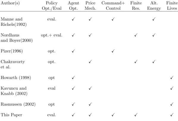
series of potential scenarios. In these models, economic variables such as tax or permit levels, or control ratios are set exogenously. Policy Optimization models look at the optimal policy choice within a set of policy instruments, allowing a government to endogenously determine policy according to the maximization of a social welfare function. Much of the early work on climate change economics is summarized by Weyant (1993). Kolstad and Kelly (1999a) provide a more up to date review of IAMs in the economics and environmental science literature, beginning with the work of Manne and Richels (1992) and Nordhaus (1994). Table 1 summarizes the key features of the most recent contributions to the IAM literature. Taxes and permit based policies are grouped under price mechanisms. The model proposed in this paper addresses each of these areas with the exception of alternative energy sources. Manne and Richels (1992) use the combination of a computable general equilibrium
Table 1: Features of Selected Integrated Assessment Papers
Author(s) Policy Agent Price Command+ Finite Alt. Finite Opt./Eval Opt. Mech. Control Res. Energy Lives
Manne and eval.
Richels(1992)
Nordhaus opt.+ eval.
and Boyer(2000)
Pizer(1996) opt.
Chakravorty opt.
et al.
Howarth (1998) opt
Kavuncu and eval
Knabb (2002)
Rasmussen (2002) opt
This Paper eval.
model and a global macroeconomic model to examine the costs of limiting CO2emissions. Their book only fits loosely into the IAM literature, since it does not possess the climate feedback into welfare. Their model has a very complete treatment of the energy production sector, and explicitly models the transition to cleaner energy sources. The work in this paper is updated in Manne, Mendelsohn and Richels (1995) to include a more extensive climate sub-model and damage assessment model.
Pizer (1996) examines the effect of uncertainty in a Nordhaus (1993) framework. Pizer extends upon Nordhaus’ contributions in several ways. First, the role of uncertainty in parameter values is examined, showing significant differences in optimal policies and welfare effects. Much of the effect of uncertainty is isolated on the rate of time preference. Pizer’s results suggest that there is a distribution of discount rates among agents. Second, the use of annual intervals is shown to have a significant effect on conclusions. Finally, a comparison is offered between tax and quantity regulation, the former being shown to have more positive welfare consequences.
this framework, the paper is able to examine the potential for inter-generational transfers of wealth and climate change abatement strategies to generate pareto improvements over the status quo.
Nordhaus and Boyer (2000) present a comprehensive model of climate change which allows for cross-country equilibrium prices of emissions permits. Their framework is a dynamic, deterministic model in which governments seek to maximize discounted social welfare in their country, in Nash equilibrium with other countries. Countries are able to trade emissions permits up to certain constraints. Within this framework, Nordhaus and Boyer are able to impose the constraints of the Kyoto protocol through adjusting the endowment of emissions permits in each country and restricting trade. Also important in this iteration of the model is the introduction of finite resources. Nordhaus and Boyer introduce a firm which extracts resources and provides the input to final production at extraction cost. The finite nature of the resource is captured in rising extraction costs.
Nordhaus and Boyer (2000) do not explicitly account for the substitution between energy resources over time. Rather they abstract from this using a type of composite fuel which has an emissions level corresponding to a weighted average of the emissions from all currently used sources of energy, and finite resource levels calculated in the same way. Chakravorty et al. (1997) look at the effect of endogenous substitution on future energy use profiles, and subsequently climate change. The key results of their paper are the time to complete conversion to solar energy (370 years baseline), with carbon emissions peaking in 2175. The resulting 6 degree increase in global temperature is persistent through 2275. Policy analysis conducted on the effect of taxes and research and development subsidies is done only in partial equilibrium, so it is not possible to address the growth consequences of the taxes in the model proposed. Of additional interest is the effect of the different simulations on the exhaustion rates of resources. Under the baseline simulations, all resources are extracted before the conversion to solar energy takes place. Conversely, under policy simulations which attach a tax to the use of carbon, only 8% of the remaining coal stock is exhausted. Rasmussen (2002) presents a model with 55 overlapping generations of agents. This model concentrates more on the costs of taxation to the economy than on the direct cli-mate change impacts, examining the changes to steady state growth rates arising from the imposition of a carbon tax. The results of this paper show that the consumption effects of a carbon tax are highly unequally distributed across generations, with the tax leading to decreased economic growth and long term costs to generations born far into the future.
There is no direct effect of climate on the economy however.
Kavuncu and Knabb (2002) present a model where agents live for two periods. The paper imposes a policy analogous to the Kyoto protocol and simulates the economy for approximately 350 years. It is worth noting that since a period in the model is 35 years, this only accounts for 10 model time periods. Their results are intuitive given the assumptions, showing that benefits arise only over a long time horizon and that these benefits arise sooner if more detrimental affects of climate change are assumed.
Integrated assessment models have become an important tool in the evaluation and development of environmental policy. One of the key difficulties with the application of these models has been the computational burden and complexity resulting from the large state space required to simultaneously model climate and economic variables. Kelly and Kolstad (1999b) present a background paper on the computational burdens in IAMs and present a formalized structure and methodology for solution and estimation of these models. Section 6 details an Euler equation approach to the computing of equilibria in overlapping generations models of climate change.
3
The Model
This section introduces an IAM of climate and economy made up of L = 60 overlapping generations of agents. Agents work for the first 45 periods of life, and accumulate assets to finance 15 periods of retirement. The production technology has energy as a factor which is used at an increasing rate of emissions efficiency. Use of carbon in production results in the release of carbon to the atmosphere which can affect global climate. In turn, climate state affects productivity over a long time horizon.
3.1 The Structure of the Model
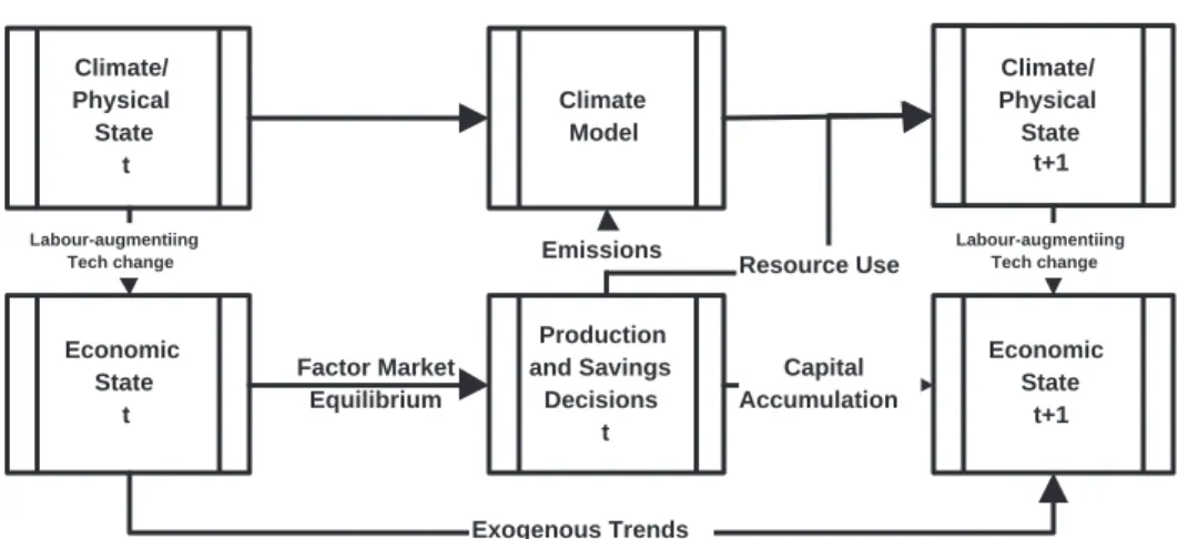
The IAM proposed below follows a three sector setup with a physical sector, an economic sector and an emissions sector. The structure of the model is denoted by mapping functions which characterize the evolution of each of the sectors of the model:
SP,t+1 = fP(SP,t, SM,t, C)
SM,t = fE(SE,t, C)
Economic State t Production and Savings Decisions t Factor Market Equilibrium Emissions Climate Model Climate/ Physical State t Labour-augmentiing Tech change Climate/ Physical State t+1 Resource Use Labour-augmentiing Tech change Economic State t+1 Capital Accumulation Exogenous Trends
Figure 1: Schematic Diagram of the Integrated Assessment Model
The interrelationships in the model are shown in the schematic diagram in Figure 1. The sectors are denoted P(physical), M(emissions), and E(economic). The model is deter-ministic. Choice variables are denoted by C. The laws of motionfi capture the relationships between sectors. In summary, next period’s physical state is affected by this period’s cli-mate, resource stocks, emissions and the choice of resource extraction. Current emissions are affected by economic state and choice variables. Next period’s economic outcome is determined by current economic and physical state, and choice variables. It is important to note that choice variables are assumed not to be able to affect climate directly, ruling out the ‘miracle solution’ where we will be able to apply new technology to change climate directly. Choice variables do affect resource extraction from the physical climate. The remainder of this section lays out in more specific detail the relationships in each section.
3.2 The Economic Environment
An initial population is spread over L generations of agents identical in all aspects except age. In each period, a large number of identical agents is born. The population grows at a convergent rate, such that population growth eventually limits to zero. In the limit therefore, there is a constant age distribution of agents. Agents in the model act to maximize their discounted stream of utility through consumption and savings paths. Agents choose consumption of a final good which is produced by competitive firms. Final good production uses carbon resources, capital and labour for which the firm pays competitive prices.
3.2.1 Agents
Agents in each generation face the same optimization problem, since they begin with the same asset holdings, have the same certain lifetimes, and face the same income. Agents choose consumption and savings to maximize their expected lifetime utility, which is given by: L i=1 βi−1U(c i,t+i−1). (2)
where β gives the agent’s discount factor β ∈ (0,1), ci,t+i−1 is consumption by an age i agent at time t+i-1. Utility has constant relative risk aversion form, with risk aversion parameterσ as:
U(ci,t+i−1) =c
1−σ i,t+i−1
1−σ . (3)
Agents accumulate assets in the form of claims on physical capital (ai,t), and use asset holdings to smooth consumption over time according to the following individual budget constraint shown in (4).
ai,t+1 = (1 +ιt−δk)ai,t+yi,t−ci,t (4)
where y is period labour income, c is consumption, and ι is the rate of return on assets from the previous period. Agents also bear the cost of depreciation δk. There is no asset bequest in the model, so agents will setaM+1,t= 0∀t. There is also a borrowing constraint in the model such that asset holdings must be aM+1,t ≥ 0 ∀t. Agents derive no utility from the bequest of environmental quality. The lack of a bequest motive is not inconsistent with the literature. In Howarth (1998), there is no consumption or environmental bequest, while in Nordhaus and Boyer (2000), an annual discount factor of .96% leads to almost no consideration outside of the time horizon of an average lifespan.1
At any point in time, an agent’s resources are the combination of asset holdings ai,t and a labour endowment ei which is age but not time dependent. The structure of the human capital profile is discussed further in Section 7. The problem of each individual in a generation is identical, so we can generalize by looking at a representative age iagent’s problem. The maximization problem for an agent is summarized by the value function given below, with the sequence of budget constraints substituted for consumption:
Vi(ai,t, t)≡amax
i+1,t+1
(A∗twitei+ (1 +ιt−δk)ai,t−ai+1,t+1)1−σ
1−σ +βVi+1(ai+1,t+1, t+ 1). (5)
The Euler equations for this problem are:
ai+1,t+1 : c−i,tσ =βV1(ai+1,t+1, t+ 1). (6)
and substituting from the envelope condition in (7) yields, for each age group, an Euler equation(8).
V1(at+1, t+ 1) =U1(ct+1) (7)
c−σ
i,t =β(1 +ιt+1−δk)c−i+1σ,t+1 (8)
Finally, substituting the budget constraint back into (8) yields a difference equation which describes the asset holdings through time subject to a sequence of prices:
(A∗twtei+ (1 +ιt−δk)ai,t−ai+1,t+1)−σ (9) =β(1 +ιt+1−δk)A∗t+1wt+1ei+1+ (1 +ιt+1−δk)ai+1,t+1−ai+2,t+2−σ. Equation (9) describes consumer behaviour as it relates to physical capital accumulation and life cycle savings decisions. Feasibility requires that aggregate consumption and net investment be less than or equal to total output in all time periods.
3.2.2 Production
Production in the economy is Cobb-Douglas with three inputs; capital, labour and resources. The representative firm faces competitive priceswt for an efficiency unit of labour,ιt for a unit of physical capital, andγt for a ton of carbon-based fuel. Technology in production is given by three parameters, overall production scale Ω, labour augmenting technical change
A∗ and energy efficiencyφ. Denoting byN the aggregate labour supplied by all agents, the
firm’s problem is therefore summarized as:
max
Kt,Nt,RtYt = F(Ωt, Kt, Nt, Rt)−wtA ∗
tNt−ιtKt−(γt)Rt (10)
= ΩtKtα[A∗tNt]1−α−θ(φtRt)θ−wtA∗tNt−ιtKt−(γt)Rt. (11) Since the firms are solving a one-period maximization problem, the solution to is described by three first order conditions:
FA∗N =wt (12)
FR=γt (13)
Resource supply is treated as in Nordhaus and Boyer (2000) by assuming that a firm provides resources competitively each period, setting price equal to marginal extraction cost. The marginal cost of extraction increases in the cumulative extraction of carbon. This is consistent with finite, scarce resources.
γt=ξ1+ξ2 Xt+Rt X∗ ξ3 (15)
The link between climate, emissions, and productivity occurs through the labour aug-menting technical change parameterA∗t:
A∗t = (1 + (D0/9)·Gt2)1−−1αAt. (16)
The intuition here is that the change in climate will lead to a lowering in our ability to use labour effectively. Examples of this change occur in the learning required for agriculture to adapt to new climatic conditions and the labour and resources used in cleanup from increased environmental disasters. Gt is the 30 year normal average surface temperature,
D0 describes damages in terms of a percentage expected reduction in GDP from a 3 degree
increase inGrelative to preindustrial levels. Damages are quadratic in temperature which is consistent with the relationship to random climatic events, proportional to the variance in temperature. The use of a feedback through labour augmenting technical change as opposed to Hicks neutral technical change is analogous to Pizer(1996). At is an exogenous trend in labour augmenting technical change, such that the exogenous trend for A is given by: At=A0 exp γa δa (1−e−δat) (17)
This law of motion is identical to that used in Pizer (1996). The exogenous trend for labour supply Nt is given by the rule for the size of the new generation born each period and retirement age R: N0t = N00 exp γn δn (1−e−δnt) (18) Nt = L−1−R i=0 Nit. (19)
3.2.3 Aggregate Laws of Motion
The two endogenous stocks in the economy are physical and resource capital, which evolve according to the actions of agents and firms. The cumulative extraction of the resource
Emissions E(t) C02 Retention Rate C0 2 Emissions Ratio Resource Use R(t) Atmospheric C02 m(t) Atmospheric C02 m(t-1) Atmospheric C0 2 Decay Rate Radiative Forcing F(t) Radiative Forcing Rate Exogenous Forcing Temperature G( t+1) O(t+1) Temperature G( t) O(t) Thermal Inertia Radiative Effect on Temp
Figure 2: Schematic Diagram of the Climate Model
stock evolves according to use as:
Xt+1 =Xt+Rt (20)
and physical capital evolves according to investment and depreciation as:
Kt+1= L
i=1
ai,t+1∗Nit (21)
3.3 The Climate and Emissions Model
The role of the climate change model is to provide a law of motion for climatic state as a function of the emission of greenhouse gases as a result of production. Other IAMs have used multi-stage processes to define this motion, at the expense of a large number of (largely irrelevant) state variables. The model proposed below uses a stylized two-stage system, where atmospheric carbon stock evolves as a function of emissions and current stock. The level of atmospheric carbon alters the level of radiative forcing (heat retention) which leads to changes in surface and ocean temperature. Damages are incurred as a result of changes in temperature relative to pre-industrial normals as described in (16).
3.3.1 The Carbon Cycle
The model presented in this paper provides a simplified characterization of the global carbon cycle. Emissions Et into the atmosphere are governed by the exogenous emissions release rate parameter φt. This parameter determines the relationship between fuel burned and emissions released into the atmosphere. Rt denotes the resource use in period t, while emissions are denotedEt.
Denoting atmospheric concentration of CO2as mt, retention rates (δe) for new emissions
Et and (δa) for current stock mt net of pre-industrial levels (mb) are factors in the law of
motion for atmospheric carbon as:
mt=mb+δeEt−1+δa(mt−1−mb). (23)
This assumes, as in Pizer (1996), that the evolution of atmospheric carbon can be ap-proximated by the decay of carbon above zero emissions levels.2 Over the transition path, what is important is providing a realistic characterization of the atmospheric half-life of carbon, which this model is able to provide. This characterization differs from Nordhaus and Boyer (2000) in the fact that a no-emissions steady state for atmospheric carbon exists at preindustrial levels mb. The reason for incorporating different sink rates for emissions and existing atmospheric carbon is that emissions are released throughout the year, and carbon sink absorption is continuous. It is natural to assume that the discrete process will imply lower average absorption for emitted carbon than atmospheric carbon.
3.3.2 Radiative Forcing and Temperature
Greenhouse gases provide a change in radiative forcing, increasing heat retention relative to the baseline for the atmosphere. Radiative forcing, Ft, is modelled as a function of atmospheric carbon as follows:
Ft =
logmt
mb
log[2] + ¯Ft (24) where the units are the relative increase in radiative forcing from pre-industrial times, and
¯
Ftis the exogenous forcing levels of other greenhouse gases. The characterization of forcing
in terms of a doubling of atmospheric CO2is standard in both the scientific and economic literature on climate change.(see Pizer (1996) or Wigley et al. (1998))
The evolution of temperature, and thus climate change, occurs through a slow warming of the world’s oceans and atmosphere, which is prevented in the short run by thermal inertia, and is modelled as a two-stage process:
Gt = λ1Gt−1+η(Ft) +ωOt−1 (25)
Ot = λ2Ot−1+ (1−λ2)Gt−1 (26)
The state variable G is surface temperature inoC relative to the pre-industrial global average for 30 year normals, while O represents the change in temperature in the world’s upper oceans, globally and seasonally averaged, since 1900. The parameter η is measured inoC and denotes the potential temperature, or long run warming from a doubling in CO2. Parameters λ1 ∈ (0,1) and λ2 ∈ (0,1) are the coefficients of autoregression in the surface and ocean temperature relationships respectively. This characterization is identical to that used in Pizer (1996) and Nordhaus and Boyer (2000). The value of Gt feeds back through (16) to generate period labour-augmenting technological change.
4
Dynamics
The model presented in this paper seeks to characterize the transition path of the economy as agents use the scarce carbon resource allocated to them. The intuition here is that the economy begins on a balanced growth path using an arbitrarily small stock of carbon energy (wood as fuel), which we can denote ¯R. The discovery of a large useful stock of exhaustible carbon resources is a shock to the economy which leads the state to follow a transition path over a long time horizon until it eventually returns to the balanced growth path. While it is important to demonstrate the existence and convergence properties of such a balanced growth path, it is the transitional path of the model which is of particular interest to this paper.
4.1 Balanced Growth
Balanced growth in this class of economy is characterized by constant rates of change for physical and economic state variables and prices in per capita terms over time. The following balanced growth path characterization relies on a growth rate of A given by γa that converges to a constant. This is shown in Proposition 1 and the exogenous trend for
At given in 17. While this paper does not model an explicit stock level, there is a level of
extraction after which the use of the stock of carbon resources in production will decline asymptotically to zero, leading to a resource input to production of ¯R. It is also important to note the population and age distribution properties of the model, which converge to a constant population and age distribution over a long time horizon. As long as population and technology level limit to a constant rate of change, and resource use above the backstop
¯
(1987) or any other standard overlapping generations model of consumption and savings. The long run behaviour of the climate sector and thus the endogenous portion of theA∗ state variable is dependent on the emissions path over time. The resource stock is used up along the transition path, so the amount used above the backstop level in each period tends to 0. With resource use tending to 0, all that is required for convergence in the climate sector is to show that emissions tend to zero, the inertia process will revert to preindustrial state at some point in the future. As resource use tends to 0, emissions also tend to zero.3
Proposition 1 The convergence of the environmental variables to preindustrial levels im-plies a unique balanced growth path with environmental variables satisfying:
E →∞ 0 (27) m →∞ 590 =mb (28) G →∞ 0 (29) O →∞ 0 (30) Proof: Immediate 4.2 Transitional Dynamics
The balanced growth path for the economy is characterized above, but relies on the eventual return of climatic state variables to pre-industrial levels, in response to the asymptotic tendency of emissions to zero. The algorithm proposed in this paper allows us to analyze the effects of policies over the transition path, from an arbitrary set of initial conditions to the balanced growth path described above, and to comment on the welfare implications for agents over these transitions. In order to define the transition paths, dynamic equilibrium must be defined for the economy in transition to a balanced growth path.
Definition 4.2.1 Equilibrium along the transition path is defined by a sequence of prices
(wt, ιt, γt)Tt=1for labour, capital and resources and time horizon T, given initial capital stock,
population, and physical state. Along the transition path, the price sequence must be such that:
1. Agents satisfy their Euler equation given in (9) and supply labour inelastically.
3It is important to note here that all climate normals are in terms that are relative to pre-industrial
times, and thus take into account the previous use of the backstop technology ¯R. Intuitively, the 590GtC concentration can be seen as the steady state level which arises in the climate sector from a long run per-period emissions of ¯R.
2. Factors are paid their marginal products
3. Factor markets for capital, labour, and resources clear.
4. Carbon resources are supplied according to their marginal private cost
5
Policy
The model admits carbon taxes and emissions quotas as policy parameters. Sequences of taxes and emissions quota levels comprise the policy space of the economy. In terms of the structure of the model, the policy sector can be seen as a fourth sector in (1) which maps policies into economic and emissions states.
5.0.1 Carbon Taxes
Carbon taxes are admitted in the model as an increment to the price charged by the carbon extraction firm for the use of resources in final production. The carbon pricing function is therefore modified to:
γt=τt+ξ1+ξ2 Xt+Rt X∗ ξ3 . (31)
where τt is the dollar/ton carbon tax rate. The model admits policies which charge the carbon tax only above a threshold level. Tax revenues are assumed to be distributed lump-sum to agents in the model, such that each agent receives as equal share of the carbon tax revenue. Denoting as ˜τt the per capita carbon tax revenue, and υ the proportion of tax revenue returned to the agent, the agent’s value function and budget constraint is therefore modified to: Vi(ai,t, t) ≡ amax i+1,t+1 (A∗twt+ (1 +ιt−δk)ai,t+υ˜τt−ai+1,t+1)1−σ 1−σ (32) + βVi+1(ai+1,t+1, t+ 1).
which then modifies the Euler equation to account for the transfer of tax income.
5.0.2 Emissions Quotas
Because of the nature of the model as a global characterization, the imposition of market-based mechanisms is per se uninformative. Quotas are introduced in the model to capture the scenario where firms are not able to pay any amount in order to increase emissions where the quota levels are binding. This differs from the tax policy introduced in the model
in that resource use is directly regulated. The supply of resources is therefore constrained by the sequence of quota levels{Q}Tt=0 as:
Rs= Rs ifφtRd(γt)< Qt Qt φt otherwise.
6
Computation
In order to solve and simulate the model, an Euler equation approach is used. In each period, agents’ Euler equations and budget constraints and firms’ first order conditions must be satisfied. Prices for labour (wt), physical capital (ιt) and resource capital (γt) determine demand and supply of each commodity. The computational algorithm uses a sequence of prices to evaluate a corresponding sequence of excess demand levels, and uses a fixed point algorithm to converge to the vector of prices which satisfies the equilibrium conditions over the entire vector from time 1..T. Given a convergence criterion, the transition path of the economy from starting values is established by the converged system of prices as follows:
Algorithm 1
Objective: Solve transition path for the climate/economy system given starting values for state variables and climate normals.
Algorithm Preliminaries: Choose a convergence criterion c and an adjustment
parame-ter λc. Choose T, the time horizon, and initial guess for price sequenceP≡(wt, ιt, γt)Tt=1.
Set prices beyond T to evolve according to balanced growth conditions.
Step 1: Solve the system of Euler equations given vector of prices for all time periods. Step 2: For each time period t, complete the following sequence of steps:
• Step 2a : Given the guess (wt, ιt, γt), compute factor supply and demand values for
resources, labour and capital in time period t. Label supply and demand vectors as
(Lst, Kts, Rst) and (Ldt, Ktd, Rtd). Supply of labour and resources are inelastic.
• Step 2b : Given the factor supplies, calculate implied emissions and carbon extraction.
Given this, update cumulative carbon extraction and temperature values using the climate and emissions module.
• Step 2c : Given new climate state variables, update labour augmenting technological
change for the next period.
Step 3: Compute the vector of percentage excess demands given by the difference between each element of the time period factor supply and demand values
Step 4: Compute a new guess of prices according to the following adjustment formula for each of the prices for each t=1..T:
wi+1 t = wit+λw Ld t−Lst Ld t ιi+1 t = ιit+λι Kd t −Kts Kd t γi+1 t = γti+λγ Rd t −Rst Rd t
and return to step 1 if the maximum excess demand value exceeds the criterion c.
Step 5: Having reached convergence criteria c, define the model as an excess demand
system as:
E ≡ (Ldt −Lst, Ktd−Kts, Rdt −Rst)Tt=1
as a function of:
P= (wt, ιt, γt)Tt=1
which is a system in 3T+T*L unknowns and 3T+T*L simultaneous equations, comprising the excess demand functions and the Euler equations of each age agent at each time period.
Use a Newton routine to compute a zero of E(P).
The final step of the algorithm provides gains only in processing time. Since the Taton-nement process converges linearly and does not make use of gradient information, the Newton-Raphson method will provide substantial acceleration gains.(see Judd (1998))
7
Calibration
In the calibration of the IAM proposed above, it is important to account for the sensitivity of simulation results to certain parameters in the climate sector. Of particular interest are the parameters linking the relationship between atmospheric CO2levels and temperature changes, and the link between temperature changes and productivity decline. The param-eters of the economic model are relatively standardized in the literature. Papers such as Pizer (1996) estimate parameters of the economic model and the elements of the climate model that can be identified with variance in the data. In response to the uncertainty over the parameters governing the effects of climate change, three scenarios are considered in
the calibration of the model. Scenarios are described as optimistic, median and pessimistic, and are calibrated to correspond with the prevalence of estimates in the literature.
7.1 Economic Sector
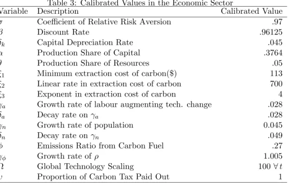
The economy is calibrated to a global production function as outlined in Pizer (1996). Baseline values for the model are 1965 economic aggregates derived from the Penn World Tables (2002). Parameters of the economic model are standard, with rates being given in annual equivalents in Table 3. Economic sector calibrations are summarized in Tables 2 and 3.
An earnings distribution is used to calibrate ei, the vector of human capital in the model, as in Huggett (1996). Data are obtained from the Canadian Labour Force Survey, 1998.4 Median wages for agents in 5 year age groups were used to construct the earnings profile, and the remaining wages were interpolated using a cubic spline. The values are adjusted so that the mean labour contribution is 1 unit. The resulting age-earnings profile is shown in Figure 4. Earnings peak from ages 45-48, which is consistent with models such as Huggett(1996) which uses U.S. data to calibrate the earnings profile.5
Growth rates are parameterized as in Nordhaus and Boyer (2000) and Howarth (1998). The calibration of population growth is accomplished by comparing the model population to patterns of population from the United Nations(UN) Population Division (2001) data and projections on world population. Population growth is initially at 4.5% in 1960, which is consistent with the fastest growth in the history of the human race taking place between 1950 and 2000. Global population limits toward a long run constant population of slightly over 10 billion people, which coincides with UN estimates of future population growth; estimates which take into account the limiting factors of density, climate, and technology. Figure 3 shows the population of agents in the model compared with UN global population estimates for people over the age of 15. Labour supply matches Penn World Tables data for the period of 1965-2000 by assuming agents retire after 45 periods. This retirement age is assumed to remain constant through time. Productivity growth in the model is parameterized in a similar way, with initial growth rates of 1.1%, converging to a constant level of technology of 153% higher than levels in the year 2000. This corresponds with the
4The Canadian data are used to generate an earnings profiles. Wage rates are determined in equilibrium,
but the difference in productivity levels by age is calibrated to the Canadian earnings profile.
5Agents enter the model at 15 years of age, and supply labour for 45 periods, retiring at the age of 60.
assumptions on the trend variables in Nordhaus and Boyer (2000) and Pizer (1996). Emissions and extraction in the model are calibrated such that emissions match global emissions data from the CDIAC (2002). This is accomplished by fixing the initial rate of energy efficiency to match 1965 emissions data, and calibrating the growth rate of efficiency to match emissions data over the time period in question. Energy efficiency is assumed to continue improving at a 1% per year rate through the simulation period of the model. Figure 5 shows the performance of the model in terms of predicting actual global carbon emissions over the 1965-2000 period.
7.2 Climate and Emissions Sectors
The fixed values in the climate sector are taken from a synthesis of five sources: Marland et al. (2002), Nordhaus and Boyer (2000), Pizer (1996), Wigley et al. (1998) and IPCC (2001). Climate sector calibrations for each of the three scenarios considered are summarized in Table 4. The key calibrated value are the retention rates for atmospheric CO2and emissions, which are derived using a first order autoregression on data from the CDIAC (2002). The model used a single parameter to represent global damages from climate change, a process which clearly has regional dimensions. This parameter is meant to capture the average decline in global productivity brought on by climate change.
8
Policy Evaluation
Models of climate change can take on two policy related roles: policy evaluation or policy optimization. This model seeks to provide a cardinal measure of the productivity and welfare costs of the transitional paths produced as a result of different implementations of mitigation strategies.
The Kyoto protocol places a target for an emissions reduction by member nations based on 1990 baseline levels to be implemented between 2008 and 2012, and the maintenance of those standards over time. This paper seeks to evaluate three policies which have been proposed as means to implement these types of CO2emissions reduction. The policies considered are the reduction of emissions to the estimated global protocol levels using a command and control quota regime, or the imposition of carbon taxes at levels which have been suggested as potential global carbon prices under Kyoto (see Government of Canada (2000,2002). Two stages of evaluation are provided. First, the three policy proposals are
compared to the status quo under median assumptions about climate change. Following this, the sensitivity of each policy’s effects to climate change assumptions is evaluated. The first policies are assumed to be continued for the entire transition path. The second set of simulations analyzes the effect of policies with a finite commitment period of fifty years after the imposition of the policies.
Policy evaluation in the model looks at three key measures. First, the overlapping generations structure allows us to look at the welfare levels for each cohort. Welfare is defined as the discounted sum of lifetime utility from consumption. The effect on the economy is measured through total output and labour productivity. Total output of the economy shows the slowdown effects of policies implemented to mitigate climate change. Aggregate productivity decline is measured through the percentage reduction in labour augmenting technical change incurred as a result of climate change. The predicted surface temperature deviations are a measure of the level of actual climate change projected by the model. Additionally, the level of cumulative carbon extraction and resulting levels of atmospheric CO2mass are secondary indicators of the success of each policy. In both cases, the economy is simulated for 380 time periods(years) with a new cohort of agents born each period (L= 60).6
8.1 Infinite Commitment
The first set of figures, labelled Figure 6 - Figure 10 show the effects of policies which remain in effect over the entire transition path under median climate change assumptions. The model predictions on welfare demonstrate one of the key issues with climate change mitigation. Figure 6 shows welfare levels for agents born in each time period of the model, under each of the policies. For agents born before 2118, the status quo is preferred to any policy. Agents born after 2118 prefer the $10 tax, but never prefer the $50 tax or the quota system.
The projected levels of final production output are shown in Figure 7. The slowdown effects of each of the policies are clearly visible in this figure. The largest single period drop in production occurs as a result of the $50 tax, with incrementally smaller changes caused by the imposition of the quota system, and the $10 tax.
6The model was simulated for a 1000 time period test to ensure that there was no perceptible difference
in the behaviour of agents on the portion of the transition path we are examining. Looking at the behaviour of the economy from the imposition of policies in 2008, there is no perceptible difference in the transition path to 2075 in a 1000 period simulation.
Productivity effects of each of the policies are shown in Figure 8. The effects are shown as percentage deviations ofA∗ from the trend variable A. Deviations are highest under the status quo of no regulation, and next highest under the tax schemes. Productivity deviation is increasing throughout the domain of the simulation.
In terms of actual changes in 30 year normal surface temperature relative to the normals for the 30 years previous to 1990, the most dramatic changes are predicted in the status quo, with temperature increase estimates of 2.42971oCover the 50 years following the imposition of policies in 2003. The evolution of surface temperatures under the status quo and each policy option are shown in Figure 9. In comparison to the status quo, the tax policies of $10/ton and $50/ton produce temperature change over the same period of 2.3596oC and 2.15441oC respectively. The quota policy is most successful in terms of climate change mitigation, showing a 50 year warming of 2.04843oC.
Figure 10 shows equilibrium in atmospheric CO2mass. Carbon use rises linearly under the quota policy, but continues to increase at an increasing rate in each time period of interest under both the tax policies and the status quo simulation. As a result, atmospheric carbon levels begin to stabilize under the quota scheme at around 920GtC, or roughly 56% above preindustrial levels. Under the status quo and tax policies, we see some evidence of convergence in the levels of atmospheric CO2as well.7
8.2 Sensitivity to Parameter Values
In order to test the sensitivity of the predictions to assumptions on the mechanism of climate change, the infinite commitment policy simulations are repeated for optimistic and pessimistic climate change assumptions, as outlined in Table 4. The ordering of the policy evaluation projections reached above are not subject to sensitivity, however the age at which agents’ preferences switch to different policies depends intuitively on the severity of climate change. In Figures 11-14, the model projections of utility, final production, productivity and temperature normals are shown under an optimistic set of climate change and damage parameters. In Figures 15-18, the same projections are reported for the more pessimistic set of parameters.
Agents’ discounted streams of utility are greatly affected by assumptions on the severity of climate change. In Figure 11, the policy preferences of agents when climate change has
7Simulating 1000 periods ahead, atmospheric CO
2levels peak and begin to drop back toward preindustrial levels under the tax policies and the status quo.
minimal effect is shown. In this simulation, welfare is never improved under the imposition of any climate change policy. Conversely, in Figure 15 we see that agents prefer more stringent regulation earlier. Agents born before 2033 prefer no regulation, while agents born between 2033 and 2056 prefer the $10/ton tax. The $50/ton tax is preferred by agents born after 2056 in the pessimistic case.
Figures 12 and 16 show the dynamics of final production under alternate climate change assumptions, while Figures 13 and 17 show the dynamics of technical change. The results here are intuitive, since we see more magnified slowdown effects as the economy is also slowed by climate change in the pessimistic scenario, with the opposite being true under the optimistic assumptions.
The most sensitivity to assumptions on climate change occurs in the projected changes in 30 year normal surface temperature. Under optimistic assumptions, temperature increase estimates of 1.42434oC over the 50 years following the imposition of policies in 2003 are recorded, compared to 3.18171oC under pessimistic assumptions. The effect of the policy
options are shown in Figures 14 and 18. The quota policy leads to a 50 year temperature increases of 1.17751oC and 2.72745oC respectively. The tax policies are projected to lead to temperature changes of 1.38025oC and 1.25099oC for the optimistic assumptions and 3.0957oC and 2.84423oC for the pessimistic case.
8.3 Sensitivity to Finite Commitment
The policy simulations are repeated in this Section, however it is assumed that the commit-ment period is 50 years, after which time the economy reverts to the status quo. Predictably, the effects of the policies on both welfare and climate are reduced by the lack of a long run change in behaviour. Figures 19-22 show the results of the finite commitment simulations. 50 years is chosen somewhat ad hoc, although the simulations are meant to frame the dis-cussion of coalition stability and the Kyoto protocol. If we consider that the regulations imposed in the Kyoto protocol might survive for 50 years, it is interesting to consider how long it will take for the economy and the climate to revert to pre-policy transition paths. This serves to examine the questions of whether it is better to undertake a less stable policy which may not last, since we feel it is important to implement some regulation.
The welfare implications of each of the policies are radically altered under the limited commitment period policies. Intuitively, agents born after the end of the commitment period prefer the most stringent policies to have been imposed previously, since these endow them
with the most productive economy. As such, agents born before the policies are implemented and until 2044 prefer that the status quo be maintained. Beyond 2045, we see that there is a rapid transition of preferences such that agents born after 2051, two years before the end of the commitment period, prefer the imposition of the most stringent quota policy.
The effects of the policies on the economy are intuitive as well. Over the commitment period, the effects are identical to those under the infinite policies. After the policies are relaxed, the economy is able to benefit from the increased productivity of a more favorable climate, and agents respond with higher levels of growth, until the economy returns to the original transition path within approximately 100 years of the end of the commitment period.
The mitigation effects are small, with the maximum temperature effects achieved at the end of the commitment period, and totalling less that 0.5oC, and disappearing all but completely within 100 years of the end of the policy. This is important since, for 50 years of large welfare effects, we have bought very little in terms of climate change mitigation. This confirms the intuition that, where we cannot be reasonably sure that the policy will be sustained for several generations, and robust to changes within the coalition, we may be better with less stringent, longer-lived policies that ensure the stability required.
9
Discussion
The question of how we measure the costs and benefits of climate change mitigation policies is a powerful one. The model and simulations presented here provide some important context to this question. First, we see clearly that, where price based mechanisms are preferred to other policies, it is important that they be set to optimal dynamic levels, not fixed over time in order to achieve maximum effectiveness and political feasibility. The simulations here show evidence of the fact that, while policies allow us to pass on a cleaner, more productive environment to future generations, these effects are tempered by the growth constraints placed on the economy by the policies. Where policies are continued indefinitely, it is only under the severest of climate change assumptions that the economy reaches higher consumption levels on the transition path than it would have under the status quo. When the policies are imposed for a finite period of time, the results are different. The reduction of emissions allows the economy to grow faster in the future, leading to higher levels of future utility. Intuitively, agents alive in the future prefer policies implemented before they
are born which improve the economic environment, but do not constrain their behaviour. The simulations shown above constitute preliminary evidence of the nature of the po-tential gains and losses to welfare under the implementation of climate change mitigating policies. In particular, the gains must be discussed in terms of welfare and productivity terms, as well as in terms of the net effect on climate. The key source of uncertainty not addressed in these measures is the cost of implementation of these measures, as the model allows the quota system to be imposed with no cost, and the tax system to fully refund all revenue to agents. Each of these also have large fixed costs to implementation which must be compared with the gains in productivity and welfare in order to determine the feasibility of a particular policy scheme. Intuitively, the majority of costs would be incurred at implementation with either the tax or quota scheme, although the quota scheme has higher enforcement costs which would be absorbed over time. The interpretation of this in the model would be a further shift outward in the preference for the status quo.
The political ramifications of these findings are clear. In order to develop a feasible climate change policy that will be accepted by today’s decision makers, accounting for future generations at some discounted rate will not be enough to induce effective mitigation policy. Some system of consumption transfers (ie. national debt) and climate policies will be required. The use of an overlapping generations model structure proves important for several reasons. First, the model is consistent with the problem of climate change. It is evident that the agents who bear a large portion of the cost of climate change policies do not directly reap any of the benefits, and this is captured in the results of the policy simulations. A representative agent model with infinitely lived agents cannot capture this feature of the problem. It can be inferred that policies with negative net benefit to agents alive at the time are not likely to be successfully imposed and continued.
References
Andolfatto, David, and Martin Gervais (1999) ‘Social security and the payroll tax with endogenous debt constraints.’ Working Paper
Andolfatto, David, Chris Ferrall, and Paul Gomme (May 2000) ‘Human capital theory and the life-cycle pattern of learning and earning, income and wealth.’ Working paper
Auerbach, A.J., and L.J. Kotlikoff (1987) Dynamic Fiscal Policy(New York, USA: Cam-bridge University Press)
Cass, D. (1965) ‘Optimum growth in an aggregate model of capital accumulation.’Review
of Economic Studies32, 233–46
Chakravorty, Ujjayant, James Roumasset, and Kinping Tse (1997) ‘Endogenous substitu-tion among energy resources and global warming.’The Journal of Political Economy
Cooley, Thomas F., and Jorge Soares (1999) ‘A positive theory of social security based on reputation.’Journal of Political Economy107(1), 135–160
Diamond, P.A. (1965) ‘National debt in a neoclassical growth model.’American Economic Review
Doornik, Jurgen A. (2003)Ox Version 3.30(Oxford)
´
Erosa, Andres, and Martin Gervais (2002) ‘Optimal taxation in life-cycle economies.’
Jour-nal of Economic Theory105, 338–369
Heckman, James J. (1976) ‘A life-cycle model of earnings, learning, and consumption.’The
Journal of Political Economy84(4), S11–S44
Heston, Alan, Robert Summers, and Bettina Aten (2002) ‘Penn World Table Version 6.1.’ Center for International Comparisons at the University of Pennsylvania (CICUP)
Howarth, Richard B. (1998) ‘An Overlapping Generations Model of Climate-Economy In-terations.’Scandinavian Journal of Ecnomics100, 575–591
Huggett, Mark (1996) ‘Wealth distribution in life-cycle economies.’ Journal of Monetary
Economics38, 469–494
Intergovernmental Panel on Climate Change (2001)Climate Change 2001(Cambridge, UK: Cambridge University Press)
Judd, Kenneth L. (1998)Numerical Methods in Economics(Cambridge, Mass., USA: Mas-sachusetts Institute of Technology)
Kavuncu, Yusuf Okan, and Shawn D. Knabb (2002) ‘An Intergenerational Cost-Benefit Analysis of Climate Change.’ Unpublished Manuscript
Kelly, David L., and Charles D. Kolstad (1999a) International Yearbook of Environmental
and Resource Economics 1999/2000: A Survey of Current Issues (Cheltenham, UK.:
Edward Elgar)
(1999b) ‘Solving growth models with an environmental sector.’ Forthcoming, Compu-tational Economics
Koopmans, Tjalling (1965) An Economic Approach to Development Planning (North Hol-land)
Manne, Alan S. (1995) ‘The rate of time preference.’ Energy Policy 23(4/5), 391–394
Manne, Alan S., and Richard Richels (1992)Buying Greenhouse Insurance: The Economic
Costs of CO2Emissions Limits(Cambridge, Mass.: The MIT Press)
Manne, Alan S., Robert Mendelsohn, and Richard Richels (1995) ‘MERGE: A model for evaluating regional and global effects of GHG reduction policies.’ Energy Policy
23(1), 17–34
Marland, G., T.A. Boden, and R. J. Andres (2002) ‘Global, regional, and national fossil fuel CO2emissions.’ In Trends: A Compendium of Data on Global Change. Carbon Dioxide Information Analysis Center, Oak Ridge National Laboratory, U.S. Department of Energy, Oak Ridge, Tenn., U.S.A.
Nordhaus, William D. (1993) ‘The Cost of Slowing Climate Change.’ Energy Journal
12(1), 37–65
(1994) Managing the Global Commons: The Economics of Climate Change (Cam-bridge, Mass.: MIT Press)
Nordhaus, William D., and Joseph Boyer (2000) Warming the World (Cambridge, Mass.: MIT Press)
Olson, Lars J., and Keith C. Knapp (1997) ‘Exhaustible resource allocation in an over-lapping generations economy.’Journal of Environmental Economics and Management
32, 277–292
Pizer, William A. (1996) ‘Modeling longterm policy under uncertainty.’ Ph.D. Thesis -Harvard University
Ramsey, Frank (1928) ‘A mathematical theory of saving.’The Economic Journal
Rasmussen, Tobias N. (2002) ‘Modelling the economics of greenhouse gas abatement: An overlapping generations perspective.’Review of Economic Dynamics
Rios-Rull, Jose Victor (1997) ‘Computation of equilibrium in heterogeneous agent models.’
Working Paper - University of Pennsylvania
T. M. L. Wigley, R. L. Smith, B. D. Santer (1998) ‘Anthropogenic influence on the auto-correlation structure of hemispheric-mean temperatures.’Science
United Nations Population Division (2001) World Population Prospects Population
Database(United Nations, New York, USA)
Weyant, John P. (1993) ‘Costs of reducing global carbon emissions.’ The Journal of Eco-nomic Perspectives
Table 2: Initial Period Values
Variable Description Calibrated Value
K0 Capital Stock 4.328∗1012
N0 Labour Supply 1.299∗109
A0 Productivity 2.5
m0 Atmospheric CO2levels 690
G0 Surface temperature change 0 O0 Ocean temperature change 0 X0 Aggregate Carbon Extraction 94 GtC
¯
F Forcings from other greenhouse gases 1.42/η ∀t
Table 3: Calibrated Values in the Economic Sector
Variable Description Calibrated Value
σ Coefficient of Relative Risk Aversion .97
β Discount Rate .96125
δk Capital Depreciation Rate .045
α Production Share of Capital .3764
θ Production Share of Resources .05
ξ1 Minimum extraction cost of carbon($) 113 ξ2 Linear rate in extraction cost of carbon 700 ξ3 Exponent in extraction cost of carbon 4
γa Growth rate of labour augmenting tech. change .028
δa Decay rate onγa .028
γn Growth rate of population 0.045
δn Decay rate onγn .049
φ Emissions Ratio from Carbon Fuel .27
γφ Growth rate ofρ 1.005
Ω Global Technology Scaling 100∀t
υ Proportion of Carbon Tax Paid Out 1
Table 4: Calibrated Values in the Climate Sector
Variable Description Sc.1 Sc.2 Sc.3
mb Preindustrial concentration of CO2 590
δa atmpspheric retention of CO2 .9846
δe atmpspheric retention of emissions .9301
λ1 AR(1) parameter on temperature deviations .9112 λ2 AR(1) parameter on ocean temperature deviations .998
η Temperature sensitivity to CO2doubling 1.5000 2.980 4.500
4 6 8 10 Population 1970 1990 2010 2030 2050 2070 2090 2110 2130 time Model Population UN Projection Figure 3: P o pulation: Mo del a nd UN Pro jection .4 .6 .8 1 1.2 1.4
Period Labour Endowment
15 30 45 60 75 age Figure 4: Earnings Profile (Pro ductivit y ratio to mean=1) 3 4 5 6 7 Emissions in GtC 1970 1980 1990 2000 time emissions2 Global Emissions Figure 5: Predicted and A ctual E missions 906 908 910 912 914 Cohort Welfare 1970 1990 2010 2030 2050 2070 time High tax−Sc 2 Low tax−Sc 2 Quota−Sc 2 Status Quo−Sc 2 Figure 6: W elfare L ev els b y cohort
−3 −2 −1 0 Production Deviations 1970 1990 2010 2030 2050 2070 2090 2110 2130 time High Tax−Sc 2 Low Tax−Sc 2 Quota−Sc 2 Status Quo−Sc 2 Figure 7: P ercen tage Deviations in P ro duction 0 .5 1 1.5 2 2.5 Productivity Deviations 1970 1990 2010 2030 2050 2070 2090 2110 2130 time High Tax−Sc 2 Low Tax−Sc 2 Quota−Sc 2 Status Quo−Sc 2 Figure 8: Pro ductivit y D ecreases 0 1 2 3
Temperature Deviations (degrees C)
1970 1990 2010 2030 2050 2070 2090 2110 2130 time High Tax−Sc 2 Low Tax−Sc 2 Quota−Sc 2 Status Quo−Sc 2 Figure 9: Median T emp erature D eviations 700 800 900 1000 1100 1200
Atmospheric Carbon Mass in GtC
1970 1990 2010 2030 2050 2070 2090 2110 2130 time High Tax−Sc 2 Low Tax−Sc 2 Quota−Sc 2 Status Quo−Sc 2 Figure 10: A tmospheric C arb o n L ev els
906 908 910 912 914 Cohort Welfare 1970 1990 2010 2030 2050 2070 time High Tax−Sc 1 Low Tax−Sc 1 Quota−Sc 1 Status Quo−Sc 1 Figure 11: W elfare L ev els b y cohort −4 −3 −2 −1 0 Production Deviations 1970 1990 2010 2030 2050 2070 2090 2110 2130 time High Tax−Sc 1 Low Tax−Sc 1 Quota−Sc 1 Status Quo−Sc 1 Figure 12: P ercen tage Deviations in P ro duction 0 .2 .4 .6 Productivity Deviations 1970 1990 2010 2030 2050 2070 2090 2110 2130 time High Tax−Sc 1 Low Tax−Sc 1 Quota−Sc 1 Status Quo−Sc 1 Figure 13: Pro ductivit y D ecreases 0 .5 1 1.5 2 Temperature Deviations 1970 1990 2010 2030 2050 2070 2090 2110 2130 time High Tax−Sc 1 Low Tax−Sc 1 Quota−Sc 1 Status Quo−Sc 1 Figure 14: Median T emp erature D eviations
906 908 910 912 914 Cohort Welfare 1970 1990 2010 2030 2050 2070 time High Tax−Sc 3 Low Tax−Sc 3 Quota−Sc 3 Status Quo−Sc 3 Figure 15: W elfare L ev els b y cohort −3 −2 −1 0 Production Deviations 1970 1990 2010 2030 2050 2070 2090 2110 2130 time High Tax−Sc 3 Low Tax−Sc 3 Quota−Sc 3 Status Quo−Sc 3 Figure 16: P ercen tage Deviations in P ro duction 0 1 2 3 4 5 6 7 8 Productivity Deviations 1970 1990 2010 2030 2050 2070 2090 2110 2130 time High Tax−Sc 3 Low Tax−Sc 3 Quota−Sc 3 Status Quo−Sc 3 Figure 17: Pro ductivit y D ecreases 0 1 2 3 4 Temperature Deviations 1970 1990 2010 2030 2050 2070 2090 2110 2130 time High Tax−Sc 3 Low Tax−Sc 3 Quota−Sc 3 Status Quo−Sc 3 Figure 18: Median T emp erature D eviations
906 908 910 912 914 Cohort Welfare 1970 1990 2010 2030 2050 2070 time $50/Ton tax−Scenario 2 $10/Ton tax−Scenario 2 5.735 GtC Quota−Scenario 2 Status Quo−Scenario 2 Figure 19: W elfare L ev els b y cohort-Finite commitmen t −3 −2 −1 0 1 Production Deviations 1970 1990 2010 2030 2050 2070 2090 2110 2130 time $50/Ton tax−Scenario 2 $10/Ton tax−Scenario 2 5.735 GtC Quota−Scenario 2 Status Quo−Scenario 2 Figure 20: P ercen tage Deviations in P ro duction-Finite com-mitmen t 0 .5 1 1.5 2 2.5 Productivity Deviations 1970 1990 2010 2030 2050 2070 2090 2110 2130 time $50/Ton tax−Scenario 2 $10/Ton tax−Scenario 2 5.735 GtC Quota−Scenario 2 Status Quo−Scenario 2 Figure 21: Sim u lated P ro ductivit y D ecreases-Finite commit-men t 0 1 2 3
Temperature Deviations (degrees C)
1970 1990 2010 2030 2050 2070 2090 2110 2130 time $50/Ton tax−Scenario 2 $10/Ton tax−Scenario 2 5.735 GtC Quota−Scenario 2 Status Quo−Scenario 2 Figure 22: Sim u lated M edian T emp erature D eviations-Finite commitmen t