with Different Data Structures: Alternative
Approaches in Comparison
Nadia Solaro, Alessandro Barbiero, Giancarlo Manzi, and Pier Alda Ferrari
Abstract In recent years, with the spread availability of large datasets from multiple sources, increasing attention has been devoted to the treatment of miss-ing information. Recent approaches have paved the way to the development of new powerful algorithmic techniques, in which imputation is performed through computer-intensive procedures. Although most of these approaches are attractive for many reasons, less attention has been paid to the problem of which method should be preferred according to the data structure at hand. This work addresses the problem by comparing the two methodsmissForestandIPCAwith a new method we developed within the forward imputation approach. We carried out comparisons by considering different data patterns with varying skewness and correlation of variables, in order to ascertain in which situations a given method produces more satisfying results.
Keywords Forward imputation • Iterative PCA • missForest • Missing data
1
Missing Data Treatment
Missing data treatment is frequently invoked when performing data analysis. There exists no field of quantitative research where missing information is not a problem, and an optimal choice of an imputation procedure should be a guarantee of
N. Solaro ()
Department of Statistics and Quantitative Methods, Università di Milano-Bicocca, Milan, Italy e-mail:[email protected]
A. Barbiero • G. Manzi • P.A. Ferrari
Department of Economics, Management and Quantitative Methods, Università di Milano, Milan, Italy
e-mail:[email protected];[email protected];[email protected]
D. Vicari et al. (eds.),Analysis and Modeling of Complex Data in Behavioral and Social Sciences, Studies in Classification, Data Analysis, and Knowledge Organization, DOI 10.1007/978-3-319-06692-9__27,
© Springer International Publishing Switzerland 2014
reliable statistical analyses. In modern missing data handling, two broad taxonomies dominate recent literature: (1) parametric and nonparametric methods; (2) single and multiple imputation (Little and Rubin2002). In parametric methods, likelihood-based procedures (e.g. the EM algorithm) are applied starting from a distributional assumption on the missing part of data in order to obtain estimates of missing values according to their generating model. Nonparametric missing data procedures are model-free methods that do not require distributional assumptions on the data. Imputation is thus performed by learning from the data structure at hand. While single imputation is concerned with the problem of assigning a single value to each missing datum, multiple imputation aims at accounting for the uncertainty implicit in the fact that the imputed values are not the actual values. This is achieved by deliberately adding sources of error during the imputation process, thus giving rise to a multitude of estimates for each missing datum from which standard errors and confidence intervals can be computed.
Among nonparametric single imputation techniques, methods based on computer-intensive iterative statistical procedures seem the most promising in producing reliable imputations. In this work, attention is specifically drawn to three different logics of imputing, based on the use of random forest (Stekhoven and Bühlmann 2012), iterative PCA (Nora-Chouteau 1974) and the forward (Ferrari et al. 2011) procedures respectively. In particular, Stekhoven and Bühlmann’s method (missForest, Stekhoven and Bühlmann2012) is an iterative technique for the imputation of continuous and/or categorical data based on a random forest, which is a random classifier introduced in the context of machine learning (Breiman
2001). The Iterative Principal Component Analysis (IPCA) (Greenacre1984; Nora-Chouteau1974) imputes missing values simultaneously by an iterative use of the principal component analysis. It has recently been subject to renewed interest as it is at the core of the multiple imputation technique with PCA, a component of a more general methodology (missMDA) introduced by Josse et al. (2011) for imputing missing data with multivariate data analysis techniques. The Forward Imputation (ForImp) by Ferrari et al. (2011) is a sequential procedure designed for extracting a latent dimension from ordinal variables in the presence of missing data. The nonlinear PCA (NLPCA) and the nearest-neighbour imputation (NNI) method are alternated in a step-by-step process that recovers the missing ordinal categories and then extracts the latent dimension.
Although grounded on distinct logics,IPCAandForImpboth depend on factorial methods, which are widely used also in contexts where the incompleteness of infor-mation requires a different approach from a purely imputation perspective. This is the case of data fusion and data grafting procedures which, allowing databases from different sources to be combined together by recovering mismatches of variables and/or units, can be regarded as special cases of missing data imputation (Aluja-Banet et al.2007; Saporta2002).
This work has two objectives. The first is to re-formulateForImpas an imputation technique for quantitative variables. Indeed, in its original versionForImpwas not expressly developed as an imputation method, but rather as a method for missing data handling in NLPCA in alternative to commonly used standard options, such as
passive treatment (Ferrari et al.2011). The second is to offer a critical comparison of the thus revisedForImpwithmissForestandIPCAbased on various configurations of quantitative data as given by different patterns of skewness and correlation of variables.
2
The Forward Imputation for Quantitative Variables
Since our goal is to re-design theForImpmethod as a pure imputation technique, we specifically focused on missing data handling in the case of quantitative variables. Accordingly, we relied on the traditional linear PCA to build up the new version of the method, which will be termed Forward Imputation with the PCA (ForImpPCA). Although the logic behindForImpPCAis very similar to the originalForImp(Ferrari et al. 2011), it is characterized by several features. Since the dimensionality reduction problem is not the primary concern, the PCA method is merely involved as a tool functional to the imputation exercise. In particular, the same number of principal components are extracted as the number of variables in the starting data matrix, in order to produce convenient synthesis indicators that are more or less related to the original variables.
TheForImpPCAmethod assumes annpquantitative data matrix Xwithxij
values (i D1; : : : ; n; j D1; : : : ; p) with at leastprows free of missing values and the othernp rows with at mostp1 missing values (n > p; p 2). Then, in a preliminary phase, data are prepared by splittingXinto a complete submatrix X0 andK submatrices Xk, where indexk denotes the number of missing values potentially contained in each row (k D 1; : : : ; K p1). Shouldk identify a submatrix without elements, we would set:Xk D X0p, and then jump to the submatrix corresponding to the subsequentk. The core steps of the ForImpPCA algorithm are the following:
– SetkD1.
1. PCA step: Perform a PCA on the completeXk1 from either its own variance-covariance matrix or correlation matrix, assumed of full rank, and obtain eigenvalues.ks 1/ and eigenvectors!!!s.k1/ with generic element !js.k1/ from
it, (j; sD1; : : : ; p).
2. PPC step: Compute so-called Pseudo Principal Components (PPC) for both the complete Xk1 and the incomplete Xk by involving only common variables without missing values and eigenvectors obtained at the previous step, in order to obtain artificial variables free of missing values for both complete and incomplete units. We denote bythe set formed by those among thek-combinations of the
pindices of variables containing missing values in the rows ofXk. Then PPCs, denoted byCQ, are given by linear combinations of the original variables outside theset with coefficients given by the element in the corresponding eigenvectors:
Q
Cs./.k/ DPplD1
l…
!ls.k1/Xl.k/for submatrixXk, and:CQs./.k1/ D Pp
lD1 l…
!ls.k1/Xl.k1/
for submatrixXk1,sD1; : : : ; p.
3. Donors’ selection step: PPCs represent common, complete information for the comparison of complete and incomplete units. PPCs are accordingly used to compute the Minkowski distance dr of order r, .r 1/, between each incomplete unitu.k/i inXkand the complete unitsuc.k1/inXk1:
dr.u.k/i ;u.kc1//D ( p X sD1 ˇˇ ˇ.cQs./;i.k/ Qcs./;c.k1//w.ks 1/ˇˇˇr )1=r ; cD1; : : : ; nk1; (1)
where the weights:w.ks 1/ D q
.ks 1/=
Pp mD1
.k1/
m , being the square root of normalized eigenvalues, are used to strengthen (weaken) the role of PPCs derived from principal components with higher (smaller) variances. Thereafter, donors are detected as an opportune percentage of the complete units nearest to a specific incomplete unit. Formally, donorsu.k/ı;i for unitu.k/i are given by the firstq100% complete unitsu.kc1/corresponding to theq-th quantiledq;iof the distancesdr,
(0 < q < 1;iD1; : : : ; nk).
4. Imputation step: Once the donors have been identified, their values in the original data matrix are used for imputation by means of a weighted average. Weights are given by the reciprocals of the distances between donors and each specific incomplete unit in order to put more (less) emphasis on less (more) distant donors. For a missing value on variableXj and unitu.k/i the imputed value is therefore given by:
Q xij.k/D Pnı ıD1x .k1/ ıj d1ıi Pnı ıD1 d1ıi ; 8j 2;
wherenı is the total number of donors foru.k/i anddıi is the distance between theı-th donor and unitu.k/i as computed in step 3.
– SetkDkC1and jump to thePCA stepuntilXis completely imputed.
3
A Data Structure-Driven Simulation Study
for Comparison
A Monte Carlo simulation study was carried out to assess the performance of the ForImpPCAmethod by comparing it withmissForest andIPCAin the presence of different data patterns and Missing Completely At Random (MCAR) generated missing values (Little and Rubin 2002). In this study, attention was specifically addressed to skewed data structures, in order to verify whether and to what extent
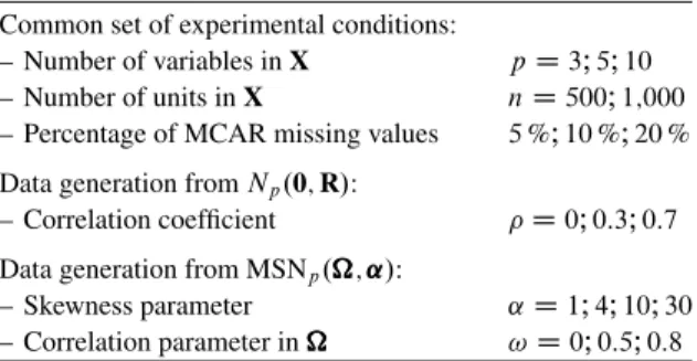
Table 1 Experimental conditions in the simulation study (1,000 runs for each scenario)
Common set of experimental conditions:
– Number of variables inX pD3I5I10 – Number of units inX nD500I1;000 – Percentage of MCAR missing values 5%I10%I20% Data generation fromNp.0;R/:
– Correlation coefficient D0I0:3I0:7 Data generation from MSNp.; ˛˛˛/:
– Skewness parameter ˛D1I4I10I30 – Correlation parameter in !D0I0:5I0:8
skewness could affect the imputation capability of the three methods. Accordingly, complete data matrices were randomly generated from both the multivariate normal (MVN) distribution and the multivariate skew normal (MSN) family of distributions, the latter being an extension of the multivariate normal distribution allowing for the presence of skewness (Azzalini and Capitanio1999; Azzalini and Dalla Valle1996). To better understand the role ofMSNparameters involved in the simulation study, it is worth recalling that ap-dimensional random vectorXXXis MSNp.; ˛˛˛/distributed if its density function (d.f.) can be expressed as:
f .xI; ˛˛˛/D2p.xI/ˆ.˛˛˛tx/; (2)
where:p.xI/is theNp.0; /d.f., witha correlation matrix of full rank;ˆ./ is the N.0; 1/ distribution function, and ˛˛˛ is a p-dimensional parameter vector regulating the skewness. In particular, if:˛˛˛ D 0, then the d.f. (2) reduces to a multivariate normal:XXX Np.0; /.
We generated data from both MVN and MSN distributions according to the simulation settings reported in Table 1, for a total number of, respectively, 54
scenarios in the case of MVN, and 216 in the case of MSN. Specifically, in each scenario a complete data matrix X was generated from an MVN or an MSN distribution, and then 1,000 matrices Xt were formed from it with a given percentage of MCAR missing data,t D 1; : : : ; 1;000(Table1). Then,missForest, IPCA andForImpPCA were applied with the following options. For missForest, the maximum number of iterations was increased from10 (the default in the R librarymissForest, Stekhoven and Bühlmann2012) to50. For IPCA, the number of extracted principal components was fixed to the maximum possible, i.e.p2, withp3(R librarymissMDA, Josse et al.2011). ForForImpPCA, we considered the Euclidean distance (r D 2 in formula (1)), and the firstq-th quantile of such distances withqD0:05I0:1I0:15I0:2in order to detect donors.
Simulation results were synthesized, and comparisons among the three methods performed, through the Relative Mean Square Error (RMSE) computed as a function of the difference between the complete data matrixXand the imputed data matrix
Q
Xtat thet-th simulation run:RMSEt D Pp
jD1n12 j.
xj Qxj; t/t.xj Qxj; t/;wherexj is thej-th column vector ofX,xQj; t is thej-th column vector ofXQt, andj2is the
variance of thej-th variable inX, (t D1; : : : ; 1;000). Codes ofForImpPCAwere implemented and simulations performed in the R environment (R Development Core Team2012).
3.1
Simulation Results
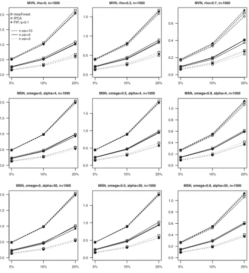
Figure1shows line plots ofRMSEmedian values, plotted against the percentages of MCAR missing values (5%I10%I20%), obtained for the three methods ( ForImp-PCAwithq D 0:1) under a subset of the scenarios considered, with the number of variables varying (p D 3I5I10), number of units fixed ton D 1;000, and data generated fromMVN (with D 0I0:3I0:7) andMSN (with! D 0I0:5I0:8 and
˛ D 4I30). The other omitted results exhibit the same trend. Two remarks are worth making. First, as expected,RMSE increases as the complexity of the data increases, that is, the number of variables and the proportion of missing values. Moreover, ceteris paribus, RMSE tends to decrease as the correlation between variables increases, thus indicating that the imputation process is more effective if variables are closely related. Second, the three methods produce very similarRMSE values with a low percentage of missing values, whereas they display a noticeably different performance in the presence of higher proportions of missing data. In particular,IPCAturns out to be the best imputation method in the case of normally distributed data (1st row of panels, Fig.1), and highly correlated variables (2nd and 3rd rows, last column, Fig.1), whileForImpPCAtends to perform best with skew distributions and variables with small/medium correlations (2nd and 3rd rows, first two columns, Fig.1). Finally,missForesttends to produce the highestRMSEvalues in most scenarios considered, although it must be remembered that it is designed especially for imputation in the case of mixed-type data.
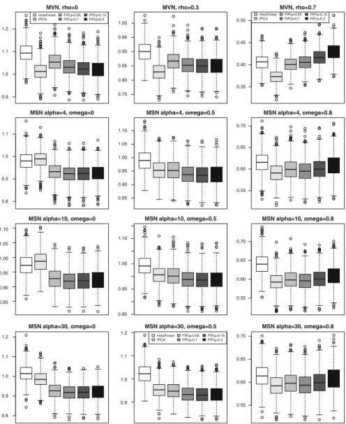
Figure2displays a more detailed picture of the results achieved in the specific scenarios withp D 5 variables,n D 1;000units, and 20% of missing data. In addition tomissForestandIPCA, boxplots ofRMSEdistributions are shown also for ForImpPCAwith different donors’ quantiles (q D 0:05I0:1I0:15I0:2), in order to check their effect on the imputation task. The above remarks concerningIPCAand ForImpPCAcan now be understood more clearly. The best performance ofIPCA can be observed in the first row of panels, while 2nd to 4th rows in the first two columns highlight the best performance ofForImpPCA. Moreover, a comparison among boxplots ofForImpPCA pertaining to different donors’ quantiles suggests that, overall, having a high percentage of donors is not a convenient choice if variables are highly correlated (last column of panels, Fig.2), while having few donors is not suitable if variables are uncorrelated or little correlated (1st column, Fig.2). This would seem to indicate that a good choice is to select donors that correspond to the firstqD0:1orqD0:15quantile of Euclidean distances.
MVN, rho=0, n=1000 missForest IPCA FIP, q=0.1 n.var=10 n.var=5 n.var=3 5% 10% 20% 0.0 0.5 1.0 1.5 2.0 MVN, rho=0.3, n=1000 5% 10% 20% 0.0 0.5 1.0 1.5 MVN, rho=0.7, n=1000 5% 10% 20% 0.0 0.2 0.4 0.6 MSN, omega=0, alpha=4, n=1000 5% 10% 20% 0.0 0.5 1.0 1.5 2.0 MSN, omega=0.5, alpha=4, n=1000 5% 10% 20% 0.0 0.5 1.0 1.5 MSN, omega=0.8, alpha=4, n=1000 5% 10% 20% 0.0 0.2 0.4 0.6 0.8 1.0 MSN, omega=0, alpha=30, n=1000 5% 10% 20% 0.0 0.5 1.0 1.5 2.0 MSN, omega=0.5, alpha=30, n=1000 5% 10% 20% 0.0 0.5 1.0 1.5 MSN, omega=0.8, alpha=30, n=1000 5% 10% 20% 0.0 0.2 0.4 0.6 0.8 1.0
Fig. 1 Line plots ofRMSEmedian values ofmissForest,IPCA, andForImpPCA(FIP), plotted against percentages of MCAR missing data withpD3I5I10variables andnD1;000units
4
Discussion and Future Work
In the light of our current results,ForImpPCA seems to be promising as a single imputation method. It performs best with skew distributions and variables which are not highly correlated, characteristics typically encountered in real data. Nonetheless, further studies would help investigate the performance ofForImpPCA more thor-oughly. For example, the results obtained indicate that it would be useful to examine ForImpPCA, and to then compare it with other methods, in the presence of data contaminations such as multivariate outliers, or a different generating mechanism of missing data, such as MAR (Little and Rubin2002). From a methodological point of
MVN, rho=0 0.9 1.0 1.1 1.2 missForest IPCA FIP,q=0.05 FIP,q=0.1 FIP,q=0.15 FIP,q=0.2 MVN, rho=0.3 0.75 0.80 0.85 0.90 0.95 1.00 MVN, rho=0.7 0.35 0.40 0.45 0.50 missForest IPCA FIP,q=0.05 FIP,q=0.1 FIP,q=0.15 FIP,q=0.2 MSN alpha=4, omega=0 0.8 0.9 1.0 1.1 MSN alpha=4, omega=0.5 0.85 0.90 0.95 1.00 1.05 1.10 MSN alpha=4, omega=0.8 0.55 0.60 0.65 0.70 MSN alpha=10, omega=0 0.85 0.90 0.95 1.00 1.05 1.10 MSN alpha=10, omega=0.5 0.80 0.90 1.00 1.10 MSN alpha=10, omega=0.8 0.55 0.60 0.65 0.70 MSN alpha=30, omega=0 0.8 0.9 1.0 1.1 1.2 MSN alpha=30, omega=0.5 0.9 1.0 1.1 1.2 missForest IPCA FIP,q=0.05 FIP,q=0.1 FIP,q=0.15 FIP,q=0.2 MSN alpha=30, omega=0.8 0.55 0.60 0.65 0.70
Fig. 2 Boxplots ofRMSEdistributions ofmissForest,IPCA, andForImpPCA(FIP) withq D
0:05; 0:1; 0:15; 0:2donors’ quantile, under the scenarios withpD5variables,nD1;000units, and20% of MCAR missing data
view, the potentially optimal properties ofForImpPCAalong with its performance in cases of more complex data structures need to be further investigated in order to highlight the capacity of ForImpPCA to manage different skew distributions better.
References
Aluja-Banet, T., Daunis-i-Estadella, J., & Pellicer, D. (2007). GRAFT, a complete system for data fusion.Computational Statistics & Data Analysis, 52, 635–649.
Azzalini, A., & Capitanio, A. (1999). Statistical applications of the multivariate skew normal distribution.Journal of the Royal Statistical Society: Series B, 61(3), 579–602.
Azzalini, A., & Dalla Valle, A. (1996). The multivariate skew-normal distribution.Biometrika, 83(4), 715–726.
Breiman, L. (2001). Random forests.Machine Learning, 45(1), 5–32.
Ferrari, P. A., Annoni, P., Barbiero, A., & Manzi, G. (2011). An imputation method for categorical variables with application to nonlinear principal component analysis.Computational Statistics & Data Analysis, 55, 2410–2420.
Greenacre, M. (1984).Theory and applications of correspondance analysis. London: Academic. Josse, J., Pagès, J., & Husson, F. (2011). Multiple imputation in principal component analysis.
Advances in Data Analysis and Classification, 5, 231–246.
Little, R. J. A., & Rubin, D. B. (2002).Statistical analysis with missing data(2nd ed.). New York: Wiley.
Nora-Chouteau, C. (1974). Une méthode de reconstitution et d’analyse de données incomplètes. Ph.D. thesis, Université Pierre et Marie Curie.
R Development Core Team (2012).R: A language and environment for statistical computing. Vienna: R Foundation for Statistical Computing.
Saporta, G. (2002). Data fusion and data grafting.Computational Statistics & Data Analysis, 38, 465–473.
Stekhoven, D. J., & Bühlmann, P. (2012). MissForest - non-parametric missing value imputation for mixed-type data.Bioinformatics, 28(1), 112–118.