Stochastic volatility with leverage: fast likelihood inference
Yasuhiro OmoriFaculty of Economics, University of Tokyo, Tokyo 113-0033, Japan [email protected]
Siddhartha Chib
Olin School of Business, Washington University, St Louis, USA [email protected]
Neil Shephard
Nuffield College, Oxford OX1 1NF, UK [email protected]
Jouchi Nakajima
Faculty of Economics, University of Tokyo, Tokyo 113-0033, Japan n [email protected]
August 22, 2004
Abstract
Kim, Shephard, and Chib (1998) provided a Bayesian analysis of stochastic volatility models based on a fast and reliable Markov chain Monte Carlo (MCMC) algorithm. Their method ruled out the leverage effect, which is known to be important in applications. De-spite this, their basic method has been extensively used in the financial economics literature and more recently in macroeconometrics. In this paper we show how the basic approach can be extended in a novel way to stochastic volatility models with leverage without altering the essence of the original approach. Several illustrative examples are provided.
Key words: Leverage effect, Markov chain Monte Carlo, Mixture sampler, Stochastic volatil-ity, Stock returns.
1
Introduction
The stochastic volatility (SV) model, a specific non-linear state space model, has been the subject of considerable attention in the econometric and statistical literatures because of the many interesting challenges it raises for estimation and inference (see, for example, the reviews in Ghysels, Harvey, and Renault (1996) and Shephard (2004)). It is also an important model because of its significance in financial applications where it has been used to understand time-varying volatility in high frequency asset returns. Kim, Shephard, and Chib (1998) developed an approach for fitting and comparing the SV model that has been extensively employed (for
example, Mahieu and Schotman (1998), Primiceri (2005) and Stroud, Muller, and Polson (2003)). This approach relies on a Bayesian Markov chain Monte Carlo (MCMC) sampling method to summarize the posterior distribution of the model parameters and the latent time varying volatilities. The approach is highly efficient in terms of the common metrics (for example inefficiency factors) that are used to study the mixing properties of sequences that are produced by the sampling algorithm. The Kim, Shephard and Chib approach, which is based on a certain approximation to a log-chisqured distribution was developed for SV models without leverage (correlation between the errors in the measurement and evolution equations). Leverage, however, is known to be important in applications. The goal of this article, therefore, is to develop the corresponding inferential methodology for SV models with leverage without altering the essence of the Kim, Shephard and Chib approach.
The simplest model we study is the well known log-normal stochastic volatility (SV) model given by
yt = ǫtexp(ht/2), (1)
ht+1 = µ+φ(ht−µ) +ηt, t= 0,1, . . . , n,
whereyt is the observed response, {ht}are unobserved log-volatilities,|φ|<1,
ǫt ηt ! ∼N(0,Σ), and Σ = 1 ρσ ρσ σ2 ! .
The parameterρmeasures the leverage effect. The leverage effect refers to the increase in volatil-ity following a drop in equvolatil-ity returns and, in this model, corresponds to a negative correlation between ǫt and ηt (e.g. Black (1976), Nelson (1991) and Yu (2004)). The latter reference also
gives a discussion of various alternative MCMC schemes put forward in the literature.
In the Kim, Shephard, and Chib (1998) approach the distribution of logǫ2t is approximated by a mixture of seven Gaussian distributions such that the first four moments of both densities are equal. They then wrote the mixture distribution hierarchically in terms of a latent compo-nent indicator (one for each time period) and conducted the MCMC sampling on the posterior distribution of the latent component indicators, the vector of latent volatilitiesh={ht}nt=1 and
the parameters. One key feature of their method is that it permits for the joint sampling of h conditioned on the latent component indicators thus leading to posterior draws that mix better than alternative approaches that rely on one-at-a time sampling of the volatilities. The sampling is finished by a reweighting step to overcome any error arising from the mixture approximation. Although this approach has proved valuable and has formed the basis of many subsequent stud-ies it was designed only for the case where ρ= 0. In this paper we show that the approach can be extended in a novel way to SV models with leverage by starting with the joint distribution of logǫ2t, ηt|sign(yt) and approximating this distribution by a suitably constructed ten-component
mixture of normal distributions. We discuss how this is done and show that it effectively solves the problems of fitting SV models with leverage. We also show how our new approach can be further extended to cover more general SV models than those given in (1).
The rest of the paper is organized as follows. In Section 2 we develop in detail our approach to dealing with SV models with leverage. Section 3 illustrates the working of this method, while in Section 4 we illustrate the methods on some data from the Japanese stock market. In Section 5 we show that the analysis extends to much wider classes of SV models, while Section 6 concludes.
2
Efficient auxiliary mixture sampler
2.1 Reformulation in the no leverage case
Following Nelson (1988) and Harvey and Shephard (1996), without loss of information we replace (1) by (dt, y∗t), the bivariate observations, where
dt = sign(yt) =I(ǫt>0)−I(ǫt≤0), (2) y∗ t = logy2t =ht+ξt, (3) and ξt= logǫ2t. Thus yt=dtexp(yt∗/2).
In the case where ρ = 0 the signs of y = (y1, ..., yn)′ are independent of y∗ = (y1∗, ..., y
∗
n)
′
and we can neglect d = (d1, ..., dn)′. This greatly simplifies the development of an inferential
methodology because y∗
is a linear process (e.g. Harvey, Ruiz, and Shephard (1994)) with an i.i.d. errorξt in (3) that follows a logχ21 density
f(ξt) = 1 √ 2πexp ξt−exp(ξt) 2 , ξt∈R.
Kim, Shephard, and Chib (1998) introduced the idea of accurately approximating this distribu-tion by a mixture of normal distribudistribu-tions, selected to ensure that moments up to a certain order are equal. In the Bayesian MCMC context, the resulting approximation error can be corrected by reweighting the sequences sampled from the posterior distribution, as we discuss below in subsection 2.3. The mixture approximation has the form of
g(ξt) = K
X
i=1
pifN(ξt|mi, vi2), ξt∈R (4)
where fN(ξt|mi, v2i) denotes the density function of a normal distribution with mean mi and
variancevi2. The constantsmi and v2i were determined by Kim, Shephard, and Chib (1998) on
the basis of K = 7 components. These values are reproduced in the first block of columns in Table 1. In this paper we have favoured a tighter approximation, based on K = 10, which is given in the second block of Table 1.
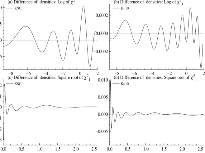
Figure 1 shows the differences between the approximate and the true densities of the logχ2 1
KSC K= 10 i pi mi v2i pi mi vi2 ai bi 1 0.04395 1.50746 0.16735 0.00609 1.92677 0.11265 1.01418 0.50710 2 0.24566 0.52478 0.34023 0.04775 1.34744 0.17788 1.02248 0.51124 3 0.34001 −0.65098 0.64009 0.13057 0.73504 0.26768 1.03403 0.51701 4 0.25750 −2.35859 1.26261 0.20674 0.02266 0.40611 1.05207 0.52604 5 0.10556 −5.24321 2.61369 0.22715 −0.85173 0.62699 1.08153 0.54076 6 0.00002 −9.83726 5.17950 0.18842 −1.97278 0.98583 1.13114 0.56557 7 0.00730 −11.40039 5.79596 0.12047 −3.46788 1.57469 1.21754 0.60877 8 0.05591 −5.55246 2.54498 1.37454 0.68728 9 0.01575 −8.68384 4.16591 1.68327 0.84163 10 0.00115 −14.65000 7.33342 2.50097 1.25049
Table 1: Selection of (pi, mi, v2i, ai, bi). Left hand side was determined by Kim, Shephard and
Chib, the ones on the right hand side are new and represent a better approximation.
andpχ21 (for the range from the 1st percentile to the 99th percentile) for the two mixtures. We can see that the move toK = 10 components improves the approximation.
−8 −6 −4 −2 0 2
−0.005 0.000 0.005 0.010
(a) Difference of densities: Log of χ21
KSC
−8 −6 −4 −2 0 2
−0.0002 0.0000 0.0002
(b) Difference of densities: Log of χ21
K=10 0.0 0.5 1.0 1.5 2.0 2.5 −0.3 −0.2 −0.1 0.0 0.1 0.2
(c) Difference of densities: Square root of χ21
KSC
0.0 0.5 1.0 1.5 2.0 2.5
−0.005 0.000 0.005
0.010 (d) Difference of densities: Square root of χ
2 1 K=10
Figure 1: The difference between the approximate and the true densities (for the range from the 1st percentile to the 99th percentile). The logχ2
1 density (top) and the p
χ2
2.2 Reformulation in general case
Now consider the general case of ρ 6= 0. The main complication is that dt is not ignorable
because, for example,
ηt|dt, ξt∼N dtρσexp (ξt/2), σ2(1−ρ2)
. (5)
Another complication is that ξt now enters both (3) and (5). To extend the approach of Kim,
Shephard, and Chib (1998) we consider the novel strategy of approximating the bivariate con-ditional density of
ξt, ηt|dt
This bivariate density is key as
(ξt, ηt|dt)⊥⊥(ξs, ηs|ds)
for all t6=s, where⊥⊥ denotes probabilistic independence. Clearly f(ξt, ηt|dt) = f(ξt|dt)f(ηt|ξt, dt)
= f(ξt)f(ηt|ξt, dt). (6)
Our idea now is to maintain the mixture approximation g(ξt) given in (4) and to consider the
approximation g(ξt, ηt|dt) = K X i=1 pifN(ξt|mi, v2i)fN ηt|dtρσexp(mi/2){ai+bi(ξt−mi)}, σ2(1−ρ2) , (7)
where (ai, bi) are known constants. In other words, we utilize a mixture of bivariate Gaussian
densities to approximate the distribution ofξt, ηt|dt. The remaining question is the determination
of the density
fN
ηt|dtρσexp(mi/2){ai+bi(ξt−mi)}, σ2(1−ρ2)
to well approximate the density of ηt|dt, ξt in the i-th component of the mixture distribution.
Due to the form of (5) this amounts to approximating exp (ξt/2) exp(−mi/2)
by
(ai+bi(ξt−mi)),
given
ξt∼N(mi, vi2).
We focus on this approximation because it does not depend upon ρ. Interestingly, ρ does not affect the quality of the approximation as we show below. We find the values of (ai, bi) by
considering the mean square norm and setting (ai, bi) = arg min
a,b E{exp (ξt/2) exp(−mi/2)−a−b(ξt−mi)}
2, ξ
By calculation we find that the solutions to this minimization problem are given by ai = exp(vi2/8), bi = E{ztexp(vizt/2)}= 1 2exp v2i 8 , i= 1,2, ..., K.
The implied values of (ai, bi) are given in Table 1.
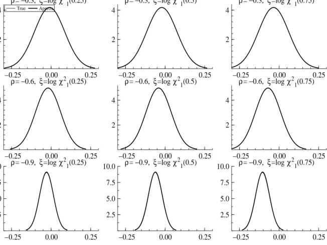
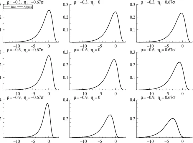
Remark 1 The key question is how well (7) approximate (6). We give results forρ=−0.3,−0.6 and −0.9. Figure 2 shows f and g for ηt|ξt, dt = 1 evaluated with ξt set at its 25th, 50th and
75th percentiles. Likewise Figure 1 shows f and g for ξt|ηt, dt= 1 evaluated with ηt=−0.67σ,
−0.25 0.00 0.25 2 4 ρ= −0.3, ξ=log χ21(0.25) True Approx −0.25 0.00 0.25 2 4 ρ= −0.3, ξ=log χ21(0.5) −0.25 0.00 0.25 2 4 ρ= −0.3, ξ=log χ21(0.75) −0.25 0.00 0.25 2 4 ρ= −0.6, ξ=log χ21(0.25) −0.25 0.00 0.25 2 4 ρ= −0.6, ξ=log χ21(0.5) −0.25 0.00 0.25 2 4 ρ= −0.6, ξ=log χ21(0.75) −0.25 0.00 0.25 2.5 5.0 7.5 10.0 ρ= −0.9, ξ=log χ 2 1(0.25) −0.25 0.00 0.25 2.5 5.0 7.5 10.0 ρ= −0.9, ξ=log χ 2 1(0.5) −0.25 0.00 0.25 2.5 5.0 7.5 10.0 ρ= −0.9, ξ=log χ 2 1(0.75)
Figure 2: The conditional density of ηt given dt = 1 and vt = logχ21(0.25), logχ21(0.5), logχ21(0.75) (left, middle, right) for ρ=−0.3, −0.6, −0.9 (top, middle, bottom).
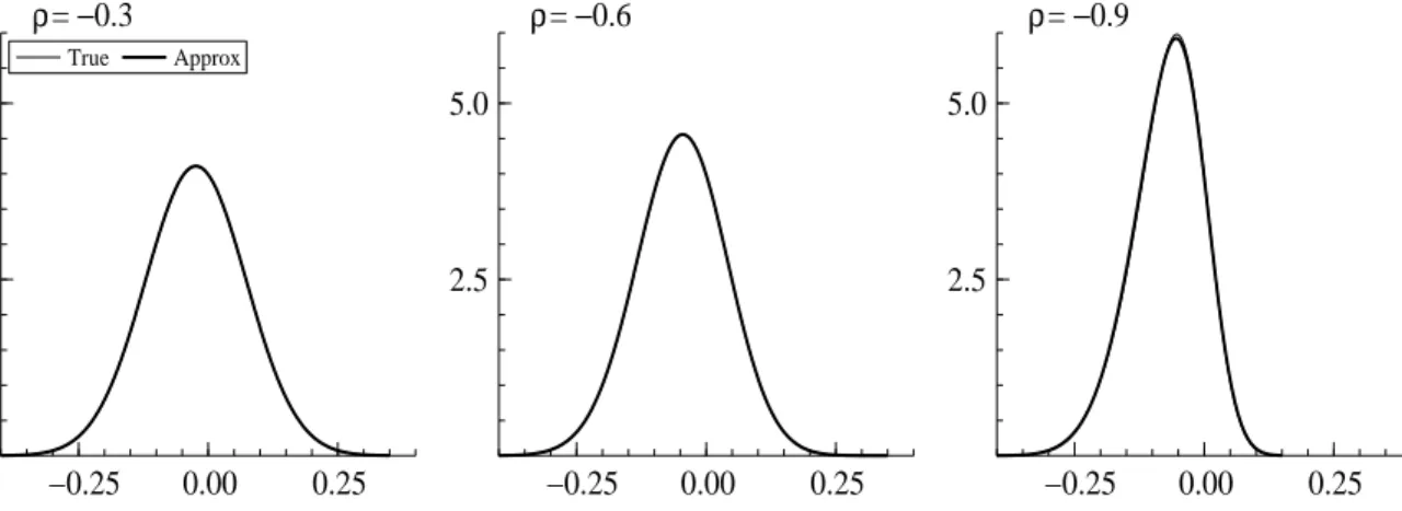
0, 0.67σ. The results suggest the approximation is quite good for it is very hard to see any difference between the true densities f and the approximations g. Further, Figure 4 shows the marginal density of ηt given dt= 1. It is clear that the true conditional joint density givendt is
−10 −5 0 0.1 0.2 0.3 ρ= −0.3, ηt= −0.67σ True Approx −10 −5 0 0.1 0.2 0.3 ρ= −0.3, ηt= 0 −10 −5 0 0.1 0.2 0.3 ρ= −0.3, ηt= 0.67σ −10 −5 0 0.1 0.2 0.3 ρ= −0.6, ηt= −0.67σ −10 −5 0 0.1 0.2 0.3 ρ= −0.6, ηt= 0 −10 −5 0 0.1 0.2 0.3 ρ= −0.6, ηt= 0.67σ −10 −5 0 0.2 0.4 ρ= −0.9, ηt= −0.67σ −10 −5 0 0.2 0.4 ρ= −0.9, ηt= 0 −10 −5 0 0.2 0.4 ρ= −0.9, ηt= 0.67σ
Figure 3: The conditional density of vt given dt = 1 and ηt =−0.67σ, 0, 0.67σ (left, middle,
right) for ρ = −0.3, −0.6, −0.9 (top, middle, bottom). The value of σ is set to 1 in this example.
2.3 MCMC algorithm
2.3.1 Broad principles
The SV model can be expressed as y∗ t ht+1 ! = ht µ+φ(ht−µ) ! + ξt ηt ! .
Now on using the mixture approximation (7) to the densityξt, ηt|dtand introducing the mixture
component indicator st∈ {1,2, ..., K}we have that
( ξt ηt ! |dt, st=i ) L = mi+vizt dtρσ(ai+bivizt) exp(mi/2) +σ p 1−ρ2z∗ t ! , zt z∗ t ! i.i.d. ∼ N(0, I).
−0.25 0.00 0.25 2.5 5.0 ρ= −0.3 True Approx −0.25 0.00 0.25 2.5 5.0 ρ= −0.6 −0.25 0.00 0.25 2.5 5.0 ρ= −0.9
Figure 4: The marginal density of ηtgiven dt= 1for ρ=−0.3,−0.6,−0.9(left, middle, right).
The value of σ is set to 1 in this example.
If we let s= (s1, ..., sn),θ= (φ, ρ, σ) and assume thatµ∼N(µ0, σ02) andh1|µ∼N(µ0, σ2/(1− φ2)), then under the auxiliary notation
e
µ1 =µe2 =...=µen=µ,
we have that the SV model with leverage can be expressed in linear Gaussian state space form (e.g. Harvey (1989), West and Harrison (1997) and Durbin and Koopman (2001))
y∗ t ht+1 e µt+1 = ht e µt+φ(ht−µet) e µt + ξt ηt 0 , (8) where h1 e µ1 ! ∼N µ0 µ0 ! , σ 2/(1−φ2) +σ2 0 σ02 σ02 σ02 !! . (9)
Under a given priorπ(θ) on θ, it is now possible to efficiently sample the posterior density
g(s, h, θ, µ|y∗
, d), where h= (h1, ..., hn), (10)
by MCMC techniques (see for example Chib (2001) for a review of these methods). Of course, this posterior is not exactly the correct one, but we will see in subsection 2.4 that it is easy to correct the small error by reweighting the sampled draws.
There are a number of different ways of sampling the posterior density above but the scheme given next is relatively simple, fast and efficient as we will show.
1. Initialize s,h,µand θ.
2. Samples|h, µ, θ, y∗
, d.
3. Sample (h, µ, θ)|s, y∗
(a) Sampling θ|s, y∗ , d. (b) Sampling µ, h|θ, s, y∗ , d. 4. Go to 2. 2.3.2 Step 2 We first define ξt=yt∗−ht, ηt= (ht+1−µ)−φ(ht−µ),
then evaluate for eachi= 1,2, ..., K
π(st = i|h, µ, θ, y∗, d) ∝ π(st=i|ξt, ηt, dt, µ, θ) ∝ Pr(st=i)v−i 1exp ( −(ξt−mi) 2 2vi2 − [ηt−dtρσexp(mi/2){ai+bi(ξt−mi)}]2 σ2(1−ρ2) ) .
This discrete distribution is sampled by the inverse distribution method.
2.3.3 Step 3
In Step 3a we sample the density
π(θ|s, y∗
, d)∝g(y∗
|d, s, θ)π(θ), marginalized over µ. The density g(y∗
|d, s, θ) is found from the output of the Kalman filter recursions applied to the model in (8) and (9). As one of the elements of the state vector is µ, which is time-invariant, this density can also be computed by the so-called augmented Kalman filter (e.g. Durbin and Koopman (2001)) but this procedure is computationally more involved. For the sampling we rely on the Metropolis-Hastings algorithm with a proposal density based on a Laplace approximation of π(θ|s, y∗
, d) (e.g. Chib and Greenberg (1995)). We define θb= ( ˆφ,σb2,ρˆ)′
which maximizes (or approximately maximizes) g(y∗
|d, s, θ)π(θ). Then we generate a candidate γ∗
from the truncated normal distribution, TNR(θ,bΣ∗), where
Σ−1 ∗ =− ∂2logg(y∗ |d, s, θ)π(θ) ∂θ∂θ′ θ=bθ ,
and R = {γ : |φ| < 1, σ2 > 0,|ρ| < 1}. Alternatively, we may generate a candidate using a transformation θ1 = log(1 +φ)−log(1−φ), θ2 = logσ21, θ3 = log(1 +ρ)−log(1−ρ). The proposal values are accepted or rejected according to the Metropolis-Hastings probability of move. When the Hessian matrix is not be negative definite (e.g. when |ρˆ| ≈1), we take a flat proposalµ∗ =θband Σ∗ =c0I using some constant c0.
Step 3b, the sampling of g(h, µ|d, s, θ), is simple and is implemented with the help of the Gaussian simulation smoother (Fr¨uhwirth-Schnatter (1994), Carter and Kohn (1994), de Jong
and Shephard (1995) and Durbin and Koopman (2002)). Software for carrying out Gaussian simulation smoothing is widely available (Koopman, Shephard, and Doornik (1999)).
2.4 Correcting for misspecification
In our approach we approximate the true bivariate density f(ξt, ηt|dt, θ) with our convenient
mixture density g(ξt, ηt|dt, θ). Thus the draws from our MCMC procedure
hj, µj, θj, j= 1,2, ..., M,
are from the approximate posterior density g(h, µ, θ|y∗
, d). To produce draws from the correct posterior densityf(h, µ, θ|y∗
, d) we simply re-weight the sampled draws. Define
ξtj =y∗
t −hjt, ηjt = (hjt+1−µj)−φj(h
j t−µj).
Then we compute the weights w∗ j = n Y t=1 f(ξjt, ηtj|dt, θj) g(ξtj, ηjt|dt, θj) , j= 1,2, ..., M, and let wj = w∗ j PM i=1w ∗ i .
We can now produce a sample from f(h, µ, θ|y∗
, d) by resampling the sampled variates with weights proportional to wj. Furthermore, posterior moments can be computed by weighted
averaging of the MCMC draws. We will see in the Monte Carlo experiments and in the em-pirical work that the variance of these weights is small, a consequence of the accuracy of our approximation, and so the effect of reweighting is modest.
2.5 Associated particle filter
In order to complete our inferential approach for this model we discuss a simulation-based approach to filtering. In particular, we show how we can recursively sample the distributions ht|y1, ..., yt,ht+1|y1, ..., ytand yt+1|y1, ..., yt, all conditional onµ, σ, ρ, φ. These sampled variates
allow us to calculate marginal likelihoods, Bayes factors and goodness of fit statistics. The filtering and the associated computations are carried out by particle filter methods (e.g., in this context, Kim, Shephard, and Chib (1998) and Pitt and Shephard (1999) or more generally Doucet, de Freitas, and Gordon (2001)).
To implement particle filtering it is helpful to define the state as αt = (ht+1, ht) in which
case the SV model with leverage can be expressed in the form of a non-linear, non-Gaussian state space model with measurement density
where
ηt= (ht+1−µ)−φ(ht−µ),
and evolution equations ht+2 ht+1 ! = µ(1−φ) 0 ! + φ 0 1 0 ! ht+1 ht ! + ηt+1 0 ! . (12)
Our particle filtering method, which we now describe, is based on draws from (12) followed by evaluations of the density in (11).
1. Initialize t= 0, αi0 from its unconditional distribution fori= 1,2, ..., I.
2. For eachisimulate
αi,jt+1|αit, j = 1,2, ..., J, (13) and computewi,j =f(yt+1|αi,jt+1) and Wi,j =F(yt+1|αti,j+1). Record
wt+1 = 1 IJ J X j=1 I X i=1 wi,j, Wt+1 = 1 IJ J X j=1 I X i=1 Wi,j.
3. Resampleαi,jt+1 with probabilities proportional towi,j to produce a sample of sizeI, which
we label as α1t+1, α2t+1, ..., αIt+1.
4. Incrementt and go to 2.
It can be shown that as I, J → ∞,wt+1
p
→f(yt+1|y1, ..., yt), and Wt+1
p
→ F(yt+1|y1, ..., yt),
the predictive distribution function. In addition, the draws onαt+1are particles fromαt+1|y1, ..., yt,
while the resampled items at stage 3 are samples fromαt+1|y1, ..., yt+1. It therefore follows that
n X t=1 logwt p → n X t=1 logf(yt|y1, ..., yt−1, µ, σ, ρ, φ),
is a consistent estimate of the conditional log-likelihood and can be used as an input in the calculation of the marginal likelihood by the method of Chib (1995). Likewise the sequence of Wt, and its reflected version 2
Wt−1/2
, can be used to check for model fit as these are approximately i.i.d. standard uniform if the model is correctly specified. This diagnostic was introduced into econometrics by Kim, Shephard, and Chib (1998), while earlier work along these lines in statistics include Shephard (1994), Smith (1985) and Rosenblatt (1952). Diagnostic checking of this type has been further popularized by Diebold, Gunther, and Tay (1998).
3
Illustrative example
This section gives illustrative examples to show the performance of the approximation discussed above. In the examples, we usey∗
t = log(yt2+c) where the offsetcis introduced to deal with very
small values of y2
approximation provides an improved fit to the left tail of the logχ21 density we set c equal to 0.0001 which is smaller than the value ofc= 0.001 used by KSC.
We simulated the data from the stochastic volatility model (1) by letting φ = 0.97, β ≡ exp(µ/2) = 0.65, σ = 0.15 and ρ=−0.3. These values are based on the estimates reported by KSC and Yu (2004) in their analysis of daily returns on foreign exchange rates and the S&P500 index. In addition, we also consider models withρ= 0,−0.6,−0.9 to investigate the effect of ρ on the quality of our inferences. In each case, we consider samples withn= 1,000 observations.
The results are based on the prior distribution µ ∼ N(0,1), φ+ 1 2 ∼Beta(20,1.5), σ−2 ∼ Gamma 5 2, 0.05 2 , ρ∼U(−1,1),
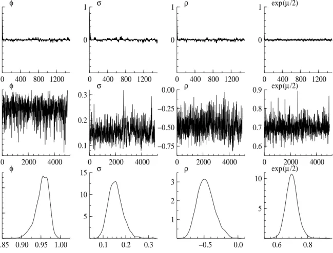
whereU(−1,1) denotes a uniform distribution on (−1,1).In the MCMC sampling of the poste-rior distribution, the initial 500 variates are discarded and the subsequentM = 5,000 values are retained for purposes of analysis. Figure 3 shows the sample paths, the sample autocorrelations function and the posterior densities of parameters for the caseρ=−0.3.The sample paths look stable and the sample autocorrelations decay quickly. In Table 2, the summary statistics are given for the cases ρ =−0.3,−0.6 and −0.9. The posterior means are close to the true values, and all true values are contained in the 95% credible intervals.
To measure how well the chain mixes, we calculate the inefficiency factors. The inefficiency factor (equivalently the autocorrelation time) is defined as 1 + 2P∞
s=1ρswhereρsis the sample autocorrelation at lags calculated from the sampled values. In KSC, where theρ= 0 case was considered, the inefficiency factors were in the range 30 ∼150 (Table 5, KSC) for the original mixture sampler and 10 ∼ 16 for the improved integration sampler (Table 6, KSC). In our MCMC implementation, these values are still small forρ =−0.3,−0.6 and −0.9, showing that our sampler is highly effective.
In order to judge the quality of our approximation we next report the distribution of the weights as discussed above. Figures 3 and 7 shows the distribution of log(w(i)×M), which would all have been zero if the approximation were exact. Figure 3 looks at the case of ρ = 0 and compares theK = 7 component analysis advocated by Kim, Shephard, and Chib (1998) to our more refined K = 10 component analysis. While the standard deviation of the log-weights based onK = 7 is 0.92, it is 0.05 whenK= 10. Kim, Shephard, and Chib (1998) demonstrated that reweighting had little impact on posterior inference about θ, µ, so we would expect that the improvement here is gratifying but small from a practical viewpoint.
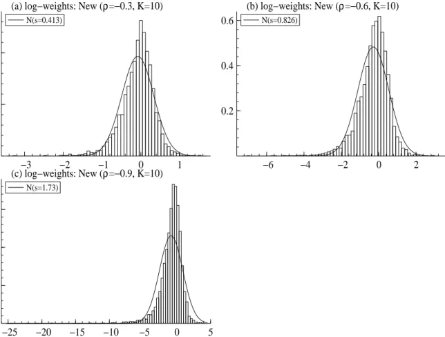
In Figure 7, the distributions of log(w(i)×M) are shown for our new approximation in an asymmetric volatility model (ρ=−0.3,−0.6,−0.9).Forρ=−0.3,its standard deviation is 0.41, which is much smaller than that of KSC in the symmetric volatility model. For ρ =−0.6, the distribution is skewed to the left, and we have a slightly larger but still small standard deviation, 0.83. For ρ = −0.9, the distribution is skewed to the left and the standard deviation is 1.73. This latter case is, however, somewhat special because in our analysis of real financial data we usually find thatρ=−0.3∼ −0.5.
0 400 800 1200 0 1 φ 0 400 800 1200 0 1 σ 0 400 800 1200 0 1 ρ 0 400 800 1200 0 1 exp(µ/2) 0 2000 4000 0.90 0.95 φ 0 2000 4000 0.1 0.2 0.3 σ 0 2000 4000 −0.75 −0.50 −0.25 0.00 ρ 0 2000 4000 0.6 0.7 0.8 0.9 exp(µ/2) 0.85 0.90 0.95 1.00 10 20 φ 0.1 0.2 0.3 5 10 15 σ −0.5 0.0 1 2 3 ρ 0.6 0.8 5 10 exp(µ/2)
Figure 5: Asymmetric stochastic volatility model (ρ=−0.3).Sample autocorrelation functions, sample paths and estimated posterior densities.
4
Real data example
In this section, we apply our approximate bivariate mixture model to the stock returns data. The data are daily returns of TOPIX (Tokyo Stock Price Index), and are calculated as the differences in the logarithm of the daily closing value of TOPIX. The sample period is from January 5, 1998 through December 30, 2002 leading to a sample of 1,232 days on which the market was open. Table 3 gives the summary statistics of the data. The mean and standard deviation of the returns are −0.026 and 1.284 respectively. In addition, there were 602 days when yt>0 and 630 days whenyt≤0.
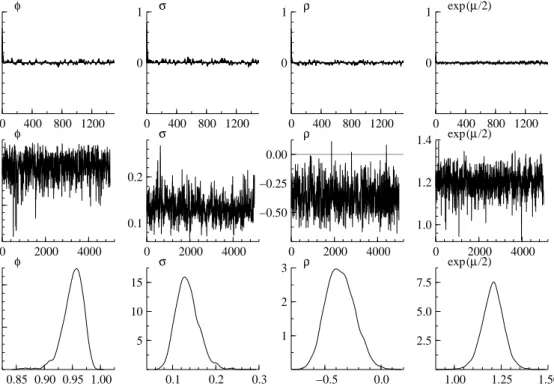
In our analysis of these data, we use the same prior distribution given above. Again as above, in the MCMC design, the initial 500 iterations are discarded and the following 5,000 values are recorded. Figure 8 shows the sample paths, the posterior densities and the sample autocorrelation functions of (φ, σ, ρ, β = exp(µ/2)). The sample autocorrelations decay quickly and the output mixes well.
Table 4 shows the estimated posterior means, standard deviations, the 95% credible intervals and inefficiency measures. Inefficiency factors are small, suggesting that 1,000 variates would
−4
−3
−2
−1
0
1
2
3
4
0.2
0.4
(a) log−weights: KSC (K=7)
N(s=0.917)−0.2
−0.1
0.0
0.1
0.2
2.5
5.0
7.5
(b) log−weights: New (K=10)
N(s=0.0535)Figure 6: Histogram of the log(w(i) ×M) where M = 5,000 is a number of samples for a symmetric stochastic volatility model (ρ = 0). Left: KSC (K = 7). Right: New (K = 10). Other line: the normal density function setting its mean and variance equal to the sample mean and sample variance.
be enough to calculate posterior moments of the parameters. The posterior means ofφ, σ, β are 0.95,0.13 and 1.21 respectively, which are typical of the values found in prior analysis of these data.
The posterior mean of ρ is −0.36 and negative as expected. Since its 95% credible interval is [−0.59,−0.11],the correlation coefficient ρ is significantly below zero. The negative value of ρ indicates that the leverage effect is present in these data.
Figure 9 shows the distributions of log(w(i) ×M) for the proposed sampler. As in the illustrative examples when ρ = −0.3, the log weights are concentrated around zero, and the standard deviation is 0.34. In contrast, Kim, Shephard, and Chib (1998) in the context of the basic SV model report a standard deviation of around 1.0 in their analysis of similar data. This shows that our overall approach is well behaved.
Table 4 shows the effect of reweighting on inference. We see that reweighting has a small effect on the estimates of the posterior mean. In the first column of Table 5 we present the log of the marginal likelihood for the SV model in theρ= 0 case. The marginal likelihood here and elsewhere was calculated by the method of Chib (1995). The log-likelihood ordinate, which is an input into this computation, was calculated from a run of the particle filter run withI = 2,500 and J = 10. The marginal likelihood of this model can be compared to the SV model with leverage given in the third column of the table. The results show that the model with leverage improves the likelihood, evaluated at the posterior mean, by around 4 at the cost of a single parameter. On the basis of the log marginal likelihood, which contains an automatic penalty for model complexity, we find that the log of the Bayes factor in favor of the leverage model is around 2.
−3 −2 −1 0 1 0.5
1.0
(a) log−weights: New (ρ=−0.3, K=10)
N(s=0.413) −6 −4 −2 0 2 0.2 0.4 0.6 (b) log−weights: New (ρ=−0.6, K=10) N(s=0.826) −25 −20 −15 −10 −5 0 5 0.1 0.2 0.3 (c) log−weights: New (ρ=−0.9, K=10) N(s=1.73)
Figure 7: Histogram of the log(w(i) ×M) where M = 5,000 is a number of samples for an asymmetric stochastic volatility model. Top right: New (ρ = −0.3, K = 10). Top left: New (ρ = −0.6, K = 10). Bottom left: New (ρ = −0.9, K = 10). Other line: the normal density function setting its mean and variance equal to the sample mean and sample variance.
5
More general dynamics
5.1 Framework
Precisely the same methods can be used to handle flexible models of the type
yt=ǫtexp(ht/2), ht=z′tαt, (14)
αt+1=bt+Ttαt+ηt, (15)
where zt, bt and Tt are non-stochastic processes, potentially dependent on some parameter θ.
We assume that ǫt ηt ! ∼N(0,Σ), Σ = 1 σ ′ σ Ω ! . (16)
In order to simplify the exposition assume that Ω is non-singular. In principle this framework can allow general forms of leverage wherein the dependence between ǫt and the elements of ηt
Unweighted Weighted
Parameter True value Mean Stdev. Mean Stdev. 95% interval Inefficiency
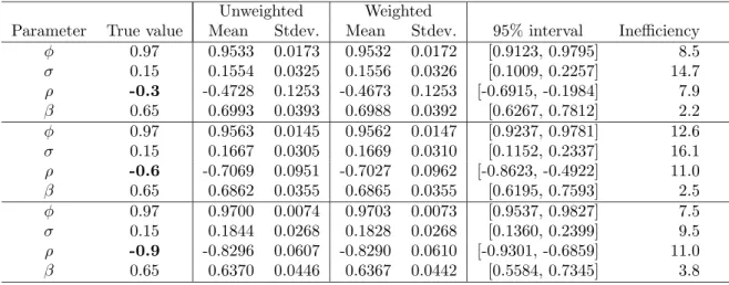
φ 0.97 0.9533 0.0173 0.9532 0.0172 [0.9123, 0.9795] 8.5 σ 0.15 0.1554 0.0325 0.1556 0.0326 [0.1009, 0.2257] 14.7 ρ -0.3 -0.4728 0.1253 -0.4673 0.1253 [-0.6915, -0.1984] 7.9 β 0.65 0.6993 0.0393 0.6988 0.0392 [0.6267, 0.7812] 2.2 φ 0.97 0.9563 0.0145 0.9562 0.0147 [0.9237, 0.9781] 12.6 σ 0.15 0.1667 0.0305 0.1669 0.0310 [0.1152, 0.2337] 16.1 ρ -0.6 -0.7069 0.0951 -0.7027 0.0962 [-0.8623, -0.4922] 11.0 β 0.65 0.6862 0.0355 0.6865 0.0355 [0.6195, 0.7593] 2.5 φ 0.97 0.9700 0.0074 0.9703 0.0073 [0.9537, 0.9827] 7.5 σ 0.15 0.1844 0.0268 0.1828 0.0268 [0.1360, 0.2399] 9.5 ρ -0.9 -0.8296 0.0607 -0.8290 0.0610 [-0.9301, -0.6859] 11.0 β 0.65 0.6370 0.0446 0.6367 0.0442 [0.5584, 0.7345] 3.8
Table 2: Summary statistics for three simulation experiments using a variety of values of ρ. Sample size is 1,000 throughout.
TOPIX (1998/1/5 - 2002/12/30)
Obs. Mean Stdev Max Min pos(+) neg(-)
1,232 -0.0255 1.2839 5.3749 -5.6819 602 630
Table 3: Summary statistics for TOPIX return data (log-difference). This structure implies that
ηt|dt, ξt∼N dtσexp (ξt/2),Ω−σσ′
.
Then, if we use our bivariate mixture approximation, we get that ( ξt ηt ! |dt, st=i ) L = mi+vizt dtσ(ai+bivizt) exp(mi/2) + (Ω−σσ′)1/2zt∗ ! , where (zt, zt∗) ′ i.i.d.
∼ N(0, I). Therefore, except for an increase in the dimension of the problem, this extension raises no new issues for our MCMC implementation.
Unweighted Weighted
Parameter Mean Stdev. Mean Stdev. 95% interval Ineff Posterior correlation
φ 0.9511 0.0185 0.9512 0.0185 [0.908, 0.980] 9.3 1 -.66 -.30 -.06
σ 0.1343 0.0262 0.1341 0.0264 [0.091, 0.193] 13.0 1 .19 -.08
ρ -0.3617 0.1265 -0.3578 0.1257 [-0.593,-0.107] 6.8 1 .13
β 1.2056 0.0573 1.2052 0.0571 [1.089, 1.318] 2.7 1
Table 4: Estimation result for TOPIX. Sample size was 5,000, based on 5,500 MCMC draws, discarding the first 500. Posterior correlation denotes the posterior correlation matrix.
0 400 800 1200 0 1 φ 0 400 800 1200 0 1 σ 0 400 800 1200 0 1 ρ 0 400 800 1200 0 1 exp(µ/2) 0 2000 4000 0.90 0.95 φ 0 2000 4000 0.1 0.2 σ 0 2000 4000 −0.50 −0.25 0.00 ρ 0 2000 4000 1.0 1.2 1.4 exp(µ/2) 0.85 0.90 0.95 1.00 10 20 φ 0.1 0.2 0.3 5 10 15 σ −0.5 0.0 1 2 3 ρ 1.00 1.25 1.50 2.5 5.0 7.5 exp(µ/2)
Figure 8: Estimation result for TOPIX. Sample autocorrelation functions, sample paths of MCMC output and estimated posterior densities.
5.2 Example: superposition model
Suppose that ht= I X i=1 αi,t, where αt+1= µ 0 0 .. . 0 + φ1 0 0 · · · 0 0 φ2 0 · · · 0 0 0 φ3 · · · 0 .. . ... ... . .. ... 0 0 0 · · · φI αt− µ 0 0 .. . 0 +ηt, and ǫt ηt ! ∼N(0,Σ), Σ = 1 ρ1σ1 ρ2σ2 · · · ρIσI ρ1σ1 σ12 0 · · · 0 ρ2σ2 0 σ22 · · · 0 .. . ... ... . .. ... ρIσI 0 σI2 .
Then the log-volatility is made up of the sum of independent autoregressions, each with a different persistence level and degree of leverage. Superposition models of this type have become popular in financial econometrics as they are more general than empirically limiting Markov
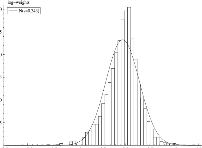
−2.5 −2.0 −1.5 −1.0 −0.5 0.0 0.5 1.0 1.5 0.25 0.50 0.75 1.00 1.25 1.50 log−weights N(s=0.343)
Figure 9: Sampling result of log-weights log(w(i)×M) for the TOPIX series. Shows histogram and fitted normal density.
volatility models while close to corresponding continuous time models (Shephard (1996), Engle and Lee (1999), Barndorff-Nielsen and Shephard (2001) and Chernov, Gallant, Ghysels, and Tauchen (2003)). It is easy to check that for Σ to be positive definite we needPIi=1ρ2
i <1.
Column 6 of Table 5 shows that for the TOPIX data set adding a second volatility component to the model has a modest effect on the fit of the model as measured by the log marginal likelihood. These results are based on a prior where (φ2 + 1)/2 ∼ Beta(10,10) with the side constraint that φ2 < φ1. Further, we assume (ρ2 + 1)/2 ∼ Beta(10,10) with the constraint that 0< ρ21+ρ22 <1. Finally, σ−2
2 ∼Gamma(5/2,0.05/2). To generate a candidate with such constraints, we may consider a transformationθ1= log(1 +φ1)−log(1−φ1), θ2= log(1 +φ2)− log(φ1 −φ2), θ3 = logσ12, θ4 = logσ22, θ5 = log(1 +ρ1)−log(1−ρ1) and θ6 = log(
p 1−ρ2 1 + ρ2)−log( p 1−ρ2
1−ρ2).Even though the log-likelihood, evaluated at the posterior mean of the parameters, is higher than the one component model, the new model has three extra parameters σ2,ρ2 and φ2, which is obviously penalized in the marginal likelihood computation.
SV SV-t ASV ASV-t ASV-g SP Likelihood ordinate -2033.98 -2033.24 -2029.85 -2029.30 -2028.87 -2029.75 (S.E.) (0.38) (0.33) (0.54) (0.48) (0.57) (0.25) Prior ordinate 3.75 0.16 3.09 3.38 3.38 7.84 Posterior ordinate 8.87 5.17 10.25 12.50 12.50 14.81 (S.E.) (0.02) (0.20) (0.02) (0.04) (0.04) (0.04) Marg Likelihood -2039.10 -2038.24 -2037.00 -2038.41 -2037.98 -2036.72 (S.E.) (0.38) (0.39) (0.54) (0.49) (0.57) (0.25)
Table 5: Marginal likelihood estimation by the Chib (1995) method for the TOPIX data. All values are in the natural-log scale. SV, SV-t and SV-g denote the SV models with Gaussian, student t and normal log-normal errors. ASV allowsρ6= 0. SP denotes superposition model.
5.3 Example: heavy-tailed error distribution
Many writers have followed Harvey, Ruiz, and Shephard (1994) in extending the SV model to allow for heavier tailed returns. For example, Chib, Nardari, and Shephard (2002) extended the basic Kim, Shephard, and Chib (1998) approach by letting
yt =
p
λtǫtexp(ht/2), (17)
ht+1 = µ+φ(ht−µ) +ηt, t= 0,1, . . . , n, (18)
where λt is an i.i.d. scale mixture variable and λt ⊥⊥ (ǫt, ηt). This is relevant empirically and
also maps into the literature on time-change L´evy processes and L´evy based SV models (Carr, Geman, Madan, and Yor (2003), Carr and Wu (2004) and Cont and Tankov (2004)). Papers on various inferential aspects of these models include Barndorff-Nielsen and Shephard (2003) and Li, Wells, and Yu (2004). In this subsection we will assume that
logλt∼N(−0.5τ2, τ2),
in which case λ1t/2ǫt has a normal log-normal distribution. This specification is closed in the
empirical work by assuming thatτ2 ∼Gamma(1,1).
The above model fits into the framework put forward in (14)-(16) by writing
yt = ǫtexp(ht/2), (19) ht = h∗t+1+λt, (20) h∗ t+1 = µ+φ(h ∗ t −µ) +ηt, t= 0,1, . . . , n, (21) where ǫt ηt λt ∼N 0 0 −0.5τ2 , 1 ρσ 0 ρσ σ2 0 0 0 τ2 . Therefore, this extension again raises no new inferential issues.
Table 5 gives results for the three different heavier tailed specifications. In the second column we report the results when √λtǫt follows a student-t distribution with ν degrees of
freedom, where ν ∼Gamma(16,0.8). The fit of this model is better than the basic model, but not over the leverage model. The fifth column reports the results for the Gaussian SV model which is marginally better than the student-t model. Overall, however, the simple Gaussian SV model with leverage is preferred for these data.
6
Conclusion
In this paper we have extended the Kim, Shephard, and Chib (1998) approach to SV models with leverage. This approach starts with the joint distribution of logǫ2t, ηt|sign(yt) which is
then approximated by a suitably constructed ten-component mixture of bivariate normal dis-tributions. We show that this approach, which is easy to implement and produces output that mixes well, effectively solves the problems of fitting SV models with leverage. We also show how our new approach can be further extended to cover even more general SV models such as those with heavy-tailed distributions and superposition effects. In each case, our algorithm performs as well as the original Kim, Shephard, and Chib (1998) algorithm but is applicable under wider conditions. We also discuss the computation of the marginal likelihood and Bayes factors and provide an empirical analysis of real Japanese stock return data where the SV model with leverage is preferred over competing models.
7
Acknowledgment
The authors thank Toshiaki Watanabe for his helpful comments. This work is partially supported by Seimeikai Foundation and Grants-in-Aid for Scientific Research 15500181 from the Japanese Ministry of Education, Science, Sports, Culture and Technology. The computational results are obtained using Ox (see Doornik (2001)). Shephard’s research is supported by the ESRC through the grant “High frequency financial econometrics based upon power variation.”
References
Barndorff-Nielsen, O. E. and N. Shephard (2001). Non-Gaussian Ornstein–Uhlenbeck-based models and some of their uses in financial economics (with discussion). Journal of the Royal Statistical Society, Series B 63, 167–241.
Barndorff-Nielsen, O. E. and N. Shephard (2003). Impact of jumps on returns and realised vari-ances: econometric analysis of time-deformed L´evy processes. Unpublished paper: Nuffield College, Oxford.
Black, F. (1976). Studies of stock price volatility changes. Proceedings of the Business and Economic Statistics Section, American Statistical Association, 177–181.
Carr, P., H. Geman, D. B. Madan, and M. Yor (2003). Stochastic volatility for L´evy processes. Mathematical Finance 13, 345–382.
Carr, P. and L. Wu (2004). Time-changed L´evy processes and option pricing. Journal of Financial Economics, 113–141.
Carter, C. K. and R. Kohn (1994). On Gibbs sampling for state space models.Biometrika 81, 541–553.
Chernov, M., A. R. Gallant, E. Ghysels, and G. Tauchen (2003). Alternative models of stock price dynamics. Journal of Econometrics 116, 225–257.
Chib, S. (1995). Marginal likelihood from the Gibbs output. Journal of the American Statis-tical Association 90, 1313–21.
Chib, S. (2001). Markov chain Monte Carlo methods: computation and inference. In J. J. Heckman and E. Leamer (Eds.), Handbook of Econometrics, Volume 5, pp. 3569–3649. Amsterdam: North-Holland.
Chib, S. and E. Greenberg (1995). Understanding the Metropolis-Hastings algorithm. The American Statistican 49, 327–35.
Chib, S., F. Nardari, and N. Shephard (2002). Markov chain Monte Carlo methods for gen-eralized stochastic volatility models.Journal of Econometrics 108, 281–316.
Cont, R. and P. Tankov (2004).Financial Modelling with Jump Processes. London: Chapman and Hall.
de Jong, P. and N. Shephard (1995). The simulation smoother for time series models. Biometrika 82, 339–350.
Diebold, F. X., T. A. Gunther, and T. S. Tay (1998). Evaluating density forecasts with applications to financial risk management.International Economic Review 39, 863–883. Doornik, J. A. (2001). Ox: Object Oriented Matrix Programming, 3.0. London: Timberlake
Consultants Press.
Doucet, A., N. de Freitas, and N. J. Gordon (Eds.) (2001). Sequential Monte Carlo Methods in Practice. New York: Springer-Verlag.
Durbin, J. and S. J. Koopman (2001). Time Series Analysis by State Space Methods. Oxford: Oxford University Press.
Durbin, J. and S. J. Koopman (2002). A simple and efficient simulation smoother for state space time series analysis. Biometrika 89, 603–616.
Engle, R. F. and G. G. J. Lee (1999). A permanent and transitory component model of stock return volatility. In R. F. Engle and H. White (Eds.),Cointegration, Causality, and Forecasting. A Festschrift in Honour of Clive W.J. Granger, pp. 475–497. Oxford: Oxford University Press.
Fr¨uhwirth-Schnatter, S. (1994). Data augmentation and dynamic linear models. Journal of Time Series Analysis 15, 183–202.
Ghysels, E., A. C. Harvey, and E. Renault (1996). Stochastic volatility. In C. R. Rao and G. S. Maddala (Eds.),Statistical Methods in Finance, pp. 119–191. Amsterdam: North-Holland.
Harvey, A. C. (1989). Forecasting, Structural Time Series Models and the Kalman Filter. Cambridge: Cambridge University Press.
Harvey, A. C., E. Ruiz, and N. Shephard (1994). Multivariate stochastic variance models. Review of Economic Studies 61, 247–264.
Harvey, A. C. and N. Shephard (1996). The estimation of an asymmetric stochastic volatility model for asset returns. Journal of Business and Economic Statistics 14, 429–434. Kim, S., N. Shephard, and S. Chib (1998). Stochastic volatility: likelihood inference and
comparison with ARCH models. Review of Economic Studies 65, 361–393.
Koopman, S. J., N. Shephard, and J. A. Doornik (1999). Statistical algorithms for models in state space using SsfPack 2.2. The Econometrics Journal 2, 107–166.
Li, H., M. Wells, and L. Yu (2004). A MCMC analysis of time-changed L´evy processes of stock returns. Unpublished paper: Johnson Graduate School of Management, Cornell University, Ithaca, U.S.A.
Mahieu, R. and P. Schotman (1998). An empirical application of stochastic volatility models. Journal of Applied Econometrics 16, 333–59.
Nelson, D. B. (1988). The time series behaviour of stock market volatility and returns. Un-published Ph.D.: MIT.
Nelson, D. B. (1991). Conditional heteroskedasticity in asset pricing: a new approach. Econo-metrica 59, 347–370.
Pitt, M. K. and N. Shephard (1999). Filtering via simulation: auxiliary particle filter.Journal of the American Statistical Association 94, 590–599.
Primiceri, G. (2005). Time varying structural vector autoregressions and monetary policy. Review of Economic Studies. Forthcoming.
Rosenblatt, M. (1952). Remarks on a multivariate transformation. Annals of Mathematical Statistics 23, 470–2.
Shephard, N. (1994). Partial non-Gaussian state space.Biometrika 81, 115–131.
Shephard, N. (1996). Statistical aspects of ARCH and stochastic volatility. In D. R. Cox, D. V. Hinkley, and O. E. Barndorff-Nielsen (Eds.), Time Series Models in Econometrics, Finance and Other Fields, pp. 1–67. London: Chapman & Hall.
Shephard, N. (2004). Stochastic Volatility: Selected Readings. Oxford: Oxford University Press. Forthcoming.
Smith, J. Q. (1985). Diagnostic checks of non-standard time series models. Journal of Fore-casting 4, 283–91.
Stroud, J. R., P. Muller, and N. G. Polson (2003). Nonlinear space models with state-dependent variances.Journal of the American Statistical Association 98, 377–386. West, M. and J. Harrison (1997). Bayesian Forecasting and Dynamic Models (2 ed.). New
Yu, J. (2004). On leverage in a stochastic volatility model. Journal of Econometrics. Forth-coming.