arXiv:1510.06852v2 [stat.ME] 27 Nov 2015
Correlation structure and variable selection in generalized
estimating equations via composite likelihood information criteria
Aristidis K. Nikoloulopoulos∗
Abstract
The method of generalized estimating equations (GEE) is popular in the biostatistics literature for analyzing longitudinal binary and count data. It assumes a generalized linear model (GLM) for the outcome variable, and a working correlation among repeated measurements. In this paper, we introduce a viable competitor: the weighted scores method for GLM margins. We weight the univariate score equations using a working discretized multivariate normal model that is a proper multivariate model. Since the weighted scores method is a parametric method based on likelihood, we propose composite likelihood information criteria as an intermediate step for model selection. The same criteria can be used for both correlation structure and variable selection. Simulations studies and the application example show that our method outperforms other existing model selection methods in GEE. From the example, it can be seen that our methods not only improve on GEEs in terms of interpretability and efficiency, but also can change the inferential conclusions with respect to GEE.
Key Words: AIC; BIC; Binary/Poisson regression; Composite likelihood; Generalized linear models;
Weighted scores.
1 Introduction
1.1 Motivating example
A European multi-center study has been conducted to evaluate safety and efficacy for three fixed doses of a new drug in patients with major depressive disorder. Subjects were followed during 8 weeks of treatment, starting from the beginning of the first week (baseline), and continuing with the beginning and the end for the next seven weeks. Measurements were taken at baseline (first week) and every week during treatment resulting in a maximum of 8 measurements per subject (unequal cluster sizes). The observations are coded as 1 if the Hamilton’s depression (Ham-D) value is less than or equal to80percent of the baseline value, and 0 otherwise. The primary question of interest is whether there is a change in Ham-D rating from baseline to week 7, or the final visit in the case of those leaving the study early. The covariates in this study are the treatment (active or placebo), and time in number of weeks from the baseline measurement. The study is described in full detail in [1].
We decided to follow the generalized estimating equations (GEE) method [2,3] to obtain a population-averaged interpretation and to address the correlation between subject outcomes. Some practical correla-tion structures given the sparsity of the data (all the responses are 0’s at the baseline), are independence, exchangeable, and AR(1); for the unstructured case we noted divergence of the GEE estimates towards infinity, hence this structure is not considered in this example. Table1gives the estimates and standard er-rors of the model parameters obtained using GEE under different hypothesized correlation structures. The GEE estimates/robust standard errors are calculated with the R package geepack [4]. It is obvious from the table that ignoring the actual correlation structure in the data could lead to invalid conclusions regarding the effect of treatment at reducing the depression levels in GEE analysis; e.g., for an exchangeable GEE analysis the treatment effect is statistically insignificant.
∗[email protected], School of Computing Sciences, University of East Anglia, Norwich Research
Table 1: GEE estimates (Est.), along with their standard errors (SE) under different hypothesized correlation structures for the Hamilton’s depression data.
Dependence Independence Exchangeable AR(1) Covariates Est. SE Est. SE Est. SE
Intercept -3.97 0.21 -3.67 0.24 -3.89 0.22 Treatment -0.54 0.21 -0.31 0.19 -0.53 0.20 Time 0.97 0.05 0.95 0.06 0.96 0.06
ρ 0.00 - 0.24 0.22 0.48 0.22
1.2 Background
The GEE method [2,3], which is popular in biostatistics, analyzes correlated data by assuming a gener-alized linear model (GLM) for the outcome variable, and a structured correlation matrix to describe the pattern of association among the repeated measurements on each subject or cluster. The correlations are treated as nuisance parameters; interest focuses on the statistical inference for the regression parameters. Recently, Nikoloulopoulos and colleagues[5] developed the weighted scores method for regression models with dependent data. The weighted scores method is essentially an extension of the GEE approach, since it can also be applied to families that are not in the GLM class. For concreteness, the theory was illustrated for discrete negative binomial margins; that are not in the GLM family. Due to its generality, the theory also applies to GLM margins.
In the case of dependent data with margins in the GLM family, the weighted scores method is a com-petitor to GEE, but the weight matrices are based on a plausible discretized multivariate normal (MVN) model, and the parameters of the weight matrices are interpretable as latent correlation parameters. This avoids problems of interpretation in GEE for a working correlation matrix that in general cannot be a correlation matrix of the multivariate data as the univariate means change [6,1].
The GEE is a proper methodology for regression with dependent discrete margins in the GLM class if the variable selection in the mean function modelling and the working correlation structure are correctly specified. Hence, when conducting a GEE analysis, it is essential to carefully model the correlation pa-rameters, in order to avoid a substantive loss in efficiency in the estimation of the regression parameters [7,8,9,10]. It turns out that model selection is important in longitudinal data analysis; two practical is-sues for modelling longitudinal data are (a) the selection of the correlation (dependence) structure among various parametric correlation matrices, such as exchangeable, AR(1), and unstructured, and (b) the vari-able/covariate selection in the regression model.
Two widely-used model-selection criteria are the Akaike’s Information Criterion (AIC), and the Bayesian Information Criterion (BIC). Since both are based on the likelihood and asymptotic properties of the max-imum likelihood estimator, they cannot be used in GEE, which are based on moments with no defined likelihood. There are some modifications of these criteria in GEE; they are not very powerful at choosing the correct correlation structure or the subset of covariates to be included in the regression model, pos-sibly because they are not likelihood-based. Pan [11] proposed the QIC criterion in GEE based on the quasi-likelihood constructed from the independent estimating equations. Hin and Wang [12] proposed a correlation information criterion (CIC), which is just the penalty term of QIC, and showed that, without the term that is theoretically independent of the correlation structures, CIC is more effective than QIC. Re-cently, Chen and Lazar [13] applied empirical likelihood to the selection of working correlation structures in GEE, and obtained two correlation structure criteria, the empirical AIC (EAIC) and the empirical BIC (EBIC). They have shown that EAIC and EBIC are consistently better than QIC and CIC.
The weighted scores method is a likelihood method and thus analogues of the AIC and the BIC for model and variable selection can be derived in the framework of the composite likelihood. Likelihood methods are effective in selecting the best model from a pool of candidates. This is a major advantage over GEE; GEE are based on moments and no likelihood is defined, hence AIC and BIC cannot be derived. We
propose/implement composite likelihood information criteria, developed by [14,15], as an intermediate step for correlation structure and variable selection. The proposed criteria have the similar attractive prop-erty with QIC of allowing covariate selection and working correlation structure selection using the same model selection criteria, but at the same time being likelihood-based, we demonstrate that outperform all of the aforementioned methods.
The remainder of the paper proceeds as follows. Section2provides the theory of the weighted scores method for binary and Poisson regression with dependent data. Section3presents the composite likelihood information criteria for model selection in the context of longitudinal data analysis with a GLM margin. Section4describes the simulation studies we perform to assess the performance of the composite likeli-hood information criteria in comparison with the existing criteria in GEE. In Section5we fully analyse the Hamilton’s depression data and show a potential change of the inferential conclusions with respect to GEE. We conclude with some remarks in Section6, followed by a brief section with the software details and a technical Appendix.
2 Weighted scores method using GLM
This section introduces the theory of the weighted scores method for GLM regression with dependent data. With GLM margins we have to deal only with univariate parameters that they are regression parameters, and thus we slightly differentiate ourselves from the general case in [5]. Before that, the first three sub-sections provide some background about important tools to form the weighted scores equations. These are the independent estimating equations in Subsection 2.1, the discretized multivariate normal (MVN) distribution in Subsection2.2, and the CL1 method [16] in Subsection2.3.
2.1 Independent estimating equations
For ease of exposition, letdbe the dimension of a “cluster” or “panel” and letnbe the number of clus-ters. The theory can be extended to varying cluster sizes. Letpbe the number of covariates, that is, the dimension of a covariate vectorxthat appears in the regression model isp×1.
Suppose that data are (yij,xij), j = 1, . . . , d, i = 1, . . . , n, where iis an index for individuals or clusters,jis an index for the repeated measurements or within cluster measurements. The first component of eachxij is taken as1for regression with an intercept. The univariate marginal model forYij is
f1(yij ; νij) = ( h−1(νij)yij 1−h−1(νij) 1−yij , Yij ∼Bernoulli h−1(νij) 1 yij!exp −h−1(νij) h−1(νij)yij , Yij ∼Poissonh−1(νij) ,
whereh(·)is the link function, i.e.,νij =x⊤ijβ=h(µij)withµij =E(Yij). The possible choices for the link functionh(·)for binary (logit and probit) and Poisson regression are given in Table2.
If for eachi,Yi1, . . . , Yidare independent, then the log-likelihood is
L1 = n X i=1 d X j=1 logf1(yij;νij) = n X i=1 d X j=1 ℓ1(νij, yij), (1)
whereℓ1(·) = log f1(·). The score equations forβare ∂L1 ∂β = n X i=1 d X j=1 ∂νij ∂β ∂ℓ1(νij, yij) ∂νij = n X i=1 d X j=1 xijs(1)ij (β) = 0. (2)
Letx⊤i = (x⊤i1, . . . ,x⊤id) and si(1)⊤(β) = (s(1)i1⊤(β), . . . ,s(1)id⊤(β)), then the score equations (2) can be written as g1 =g1(β) = ∂L1 ∂β = n X i=1 d X j=1 xTij s(1)ij (β) = n X i=1 xTi s(1)i (β) =0. (3)
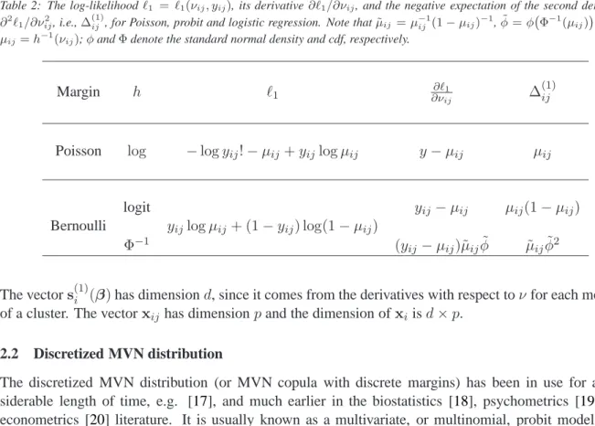
Table 2: The log-likelihoodℓ1 = ℓ1(νij, yij), its derivative ∂ℓ1/∂νij, and the negative expectation of the second derivative
∂2ℓ1/∂νij2, i.e.,∆ (1)
ij , for Poisson, probit and logistic regression. Note thatµ˜ij=µ−ij1(1−µij)−1,φ˜=φ Φ−1(µij)
,where µij=h−1(νij);φandΦdenote the standard normal density and cdf, respectively.
Margin h ℓ1 ∂ν∂ℓij1 ∆
(1) ij
Poisson log −logyij!−µij+yijlogµij y−µij µij
logit yij −µij µij(1−µij)
Bernoulli yijlogµij + (1−yij) log(1−µij)
Φ−1 (yij−µij)˜µijφ˜ µ˜ijφ˜2
The vectors(1)i (β)has dimensiond, since it comes from the derivatives with respect toνfor each member of a cluster. The vectorxij has dimensionpand the dimension ofxi isd×p.
2.2 Discretized MVN distribution
The discretized MVN distribution (or MVN copula with discrete margins) has been in use for a con-siderable length of time, e.g. [17], and much earlier in the biostatistics [18], psychometrics [19], and econometrics [20] literature. It is usually known as a multivariate, or multinomial, probit model. The multivariate probit model is a simple example of the MVN copula with univariate probit regressions as the marginals. In the general case, the discretized MVN model has the following cumulative distribution function (cdf):
Fd(y1, . . . , yd;ν1, . . . , νd,R) = Φd Φ−1[F1(y1;ν1)], . . . ,Φ−1[F1(yd;νd)];R
,
whereΦddenotes the standard MVN distribution function with correlation matrixR = (ρjk : 1 ≤ j < k ≤ d),Φis the cdf of the univariate standard normal, and F1’s are the univariate cdfs of the marginal
model for discrete data.
Implementation of the discretized MVN is feasible, but not easy, because the MVN distribution as a latent model for discrete response requires rectangle probabilities of the form
fd(yi) = Z Φ−1[F 1(yi1;νi1)] Φ−1[F1(yi1−1;νi1)] · · · Z Φ−1[F 1(yid;νid)] Φ−1[F1(y id−1;νid)] φd(z1, . . . , zd;R)dz1· · ·dzd (4)
whereφddenotes the standardd-variate normal density with correlation matrixR.
2.3 The CL1 method
The MVN copula, although inherits the dependence structure of the MVN distribution, lacks a closed form cdf; hence likelihood inference might be difficult, asd-dimensional integration is required for the computation of MVN rectangle probabilities [23,21,22]. When the joint probability is too difficult to compute, as in the case of the the discretized MVN model, composite likelihood is a good alternative [24,25].
Zhao and Joe [16] proposed the CL1 method to overcome the computational issues at the maximiza-tion routines for the MVN copula in a high-dimensional context. Estimamaximiza-tion of the model parameters can be approached by solving the estimating equations obtained by the derivatives of the composite log-likelihoods.
In addition to the the sum of univariate log-likelihoods (1) also consider the sum of bivariate log-likelihoods L2 = n X i=1 X j<k logf2(yij, yik;νij, νik, ρjk) = n X i=1 X j<k ℓ2(νij, νik, ρjk;yij, yik), where f2(yij, yik;νij, νik, ρjk) = Z Φ−1[F 1(yij;νij)] Φ−1[F1(y ij−1;νij)] Z Φ−1[F 1(yik;νik)] Φ−1[F1(y ik−1;νik)] φ2(zj, zd;ρjk)dzjdzk;
φ2(·;ρ)denotes the standard bivariate normal density with correlation ρ. Note in passing the calculation
of the bivariate normal rectangle probabilities f2(·) is straightforward and does not involve additional
computational effort as in thed-dimensional case.
Differentiating L1 with respect to βleads to the univariate composite score function or independent
estimating equations (3). Differentiating L2 with respect to R leads to the bivariate composite score
function: g2= ∂L2 ∂R = n X i=1 s(2)i (β,R) = n X i=1 s(2)i,jk(β, ρjk),1≤j < k ≤d =0, (5) where s(2)i (β,R) = ∂ P j<kℓ2(νij,νik,ρjk;yij,yik) ∂R and s (2) i,jk(β, ρjk) = ∂ℓ2(νij,νik,ρjk;yij,yik) ∂ρjk . The vector s(2)i (R)has dimension d2.
2.4 Weighted scores assuming a working multivariate model
The efficiency of estimating the regression parameters using the CL1 method can be low, since the method assumes independence. We will improve the efficiency by inserting weight matrices that depend on co-variances of the scores assuming a “working model”, such as the discretized MVN [5]. The main idea is to weight the score equations in the case of independent data within clusters or panels (3), using a working model that is actually a proper multivariate model.
To this end, the weighted scores equations for Poisson/binary regression take the form:
g1⋆=g⋆1(β) = n X
i=1
xTi W−i,working1 s(1)i (β) = 0, (6)
whereW−i,working1 = ∆(1)i (β)e Ω(1)i (βe,Re)−1 with∆(1)i (β) =e diag(∆(1)i1 , . . . ,∆(1)id ),∆(1)ij =−E (∂2ℓ1
∂ν2 ij
) andΩ(1)i (βe,Re) =Cov(s(1)i )is the the covariance matrix ofs(1)i computed assuming a working discretized MVN model with estimation approached via the CL1 method. The CL1 estimates βe for the regression parameters andRe for the correlation matrix of the discretized MVN model are obtained by solving the CL1 estimating functions in (3) and (5), respectively. The matrices∆(1)i (eβ) and Ω(1)i (βe,Re) ared×d
symmetric matrices.
The asymptotic covariance matrix of the solutionβbin (6) is
V⋆1 = (−Hg⋆ 1) −1J g⋆ 1(−H T g⋆ 1) −1, (7) with −Hg⋆ 1 = n X i=1 xTi Wi,working−1 ∆(1)i xi, Mg⋆ 1 = n X i=1
whereW−i,working1 =∆i(1)(bβ)Ω(1)i (βb,Re)−1andΩi,true(1) is the true covariance matrix ofs(1)i (β). Ω(1)i,true
can be estimated by the “sandwich” covariance estimator, that is,s(1)i (bβ)s(1)i ⊤(bβ). Explicit expressions for the elements of the log-likelihoodℓ1=ℓ1(νij, yij) = logf1(νij, yij), its derivative∂ℓ1/∂ν, and∆(1)ij , for Poisson and binary regression are given in Table2.
To summarize, the steps to obtain parameter estimates and standard errors are the following:
1. Use a discretized MVN model and estimate the parameters using the CL1 method described in the previous subsection. Let the CL1 estimates beβe for the univariate parameters andRe for the correlation matrix.
2. Compute the working weight matrices Wi,working = Ωi(βe,Re) ∆i(β)e −1, where Ωi(βe,Re) is the covariance matrix of univariate scores based on the fitted discretized MVN model.
3. Obtain robust estimatesβbof the regression parameters solving equations (6) using “working weight matrices”Wi,workingusingRe, with a reliable non-linear system solver.
4. The robust standard errors for ba are obtained calculating the estimated covariance matrix Vb⋆1 by pluggingβbforβand replacingΩi,truewithsi(ba)sTi (ba). This estimate is similar to the widely used “sandwich” covariance estimator.
The numerical methods used for various steps have been implemented in the packageweightedScores [26] within the open source statistical environmentR[27]; a wrapperRfunction is also available.
3 The CL1 information criteria
As described in the preceding section, the CL1 method in [16] is already used to estimate conveniently the univariate and latent correlation parameters of the discretized MVN model at the first step of the weighted scores method. Herein we also propose to use the CL1 method through its information criteria, for correlation structure and variable selection in the weighted scores estimating equations. The remainder of the section proceeds as follows. Subsection 3.1 provides the asymptotic covariance matrix for the estimator that solves the CL1 estimating equations. This is necessary to form the CL1 information criteria in the context of longitudinal data analysis with a GLM margin at Subsection3.2.
3.1 Asymptotic covariance matrix
The asymptotic covariance matrix for the estimator that solves (3) and (5), also known as the inverse Godambe information matrix [28], is
V= (Hg)−1Jg(H⊤g)−1, (8)
whereg= (g1,g2)⊤. First setθ= (β,R)⊤, then
−Hg =E ∂g ∂θ = E ∂g1 ∂β E∂∂g1R E∂g2 ∂β E∂g2 ∂R = −Hg1 0 −Hg1,2 −Hg2 , where−Hg1 = Pni x⊤i ∆ (1) i xi,−Hg1,2 = Pni ∆ (1,2) i xi, and−Hg2 = Pni ∆ (2,2) i . Representations of ∆(1)i ,∆i(1,2), and,∆(2)i ford= 4are given in an Appendix.
The covariance matrixJgof the composite score functionsgis given as below
Jg =Cov(g) = Cov(g1) Cov(g1,g2) Cov(g2,g1) Cov(g2) = J (1) g J(1g,2) J(2g,1) J(2)g ! =X i x⊤i Ω(1)i xi x⊤i Ω (1,2) i Ω(2i ,1)xi Ω(2)i ! ,
where, Ω(1)i Ω(1i ,2) Ω(2i ,1) Ω(2)i ! = Cov s(1)i (β) Covs(1)i (β),s(2)i (β,R) Covs(2)i (β,R),si(1)(β) Covs(2)i (β,R) .
The dimensions ofΩ(1)i ,Ω(1i ,2),Ω(2i ,1), and,Ω(2)i ared×d,d× d2, d2×d, and, d2× d2, respectively.
3.2 CL1 AIC-BIC
To this end, the CL1 AIC criterion in [14] and the CL1 BIC criterion in [15] have the forms:
CL1AIC=−2L2+ 2tr JgH−g1 , CL1BIC=−2L2+ log(n)tr JgH−g1 .
To evaluate these criteria atθˆinvolves the computation of matrices described above. The computations involve the trivariate and four-variate margins along with their derivatives. In an Appendix we provide technical and computational details for the calculation ofJg,Hgin (8), and their form for the case of one dependence parameterρ.
4 Simulations
In this section we assess the performance of the composite likelihood information criteria compared to the existing criteria in GEE.
We perform simulation studies to examine the reliability of using CL1AIC and CL1BIC to choose the correct model for longitudinal binary data. Similar results/conclusions can be expected for counts. We compare the proposed criteria with the other available criteria in GEE. In Subsection 4.1 we assess the performance of CL1AIC, CL1BIC, QIC, CIC, EAIC, and EBIC in correlation structure selection, and in Subsection4.2we investigate the performance of CL1AIC, CL1BIC, and QIC in variable selection.
4.1 Correlation structure selection
We adopt the same model considered by [11] and [13]. We randomly generateB = 103 samples of size
n= 50,100,200withd= 3using the R package bindata [29] and logistic regression withp = 3,xij = (1, x1ij, j−1)T wherex1ij are taken as Bernoulli random variables with probability of success1/2, and β0 = 0.25 =−β1 =−β2. In [11,12,13] only structured matrices were considered for the true correlation
structures. Here we consider both structured and unstructured matrices to allow for a comprehensive comparison. We consider the following choices:
• For exchangeable, we takeRas(1−0.5)I3+ 0.5O3, whereI3is the identity matrix of order3and O3is the3×3matrix of 1s.
• For AR(1),Ris taken as(0.5|j−k|)1≤j,k≤3.
• For unstructured, we takeRas 1.0 −0.5 −0.3 −0.5 1.0 0.3 −0.3 0.3 1.0 .
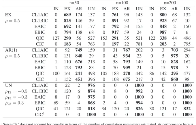
Table 3: Frequencies of the correlation structure identified using the six different criteria, namely CL1AIC, CL1BIC, EAIC, EBIC, QIC, and CIC, from 1000 simulation runs in each setting. The first column indicates the true correlation structure and its magnitude; IN, EX, and UN refer to independence, exchangeable, and unstructured correlation structure, respectively; the numbers of correct choices by each criterion are bold faced.
n=50 n=100 n=200 IN EX AR UN IN EX AR UN IN EX AR UN EX CL1AIC 0 689 174 137 0 761 96 143 0 800 68 132 ρ= 0.5 CL1BIC 0 825 146 29 0 891 92 17 0 923 67 10 EAIC 0 692 131 177 0 792 53 155 0 848 2 150 EBIC 0 794 138 68 0 917 59 24 0 987 7 6 QIC 127 290 56 527 153 291 35 521 122 338 44 496 CIC 0 183 54 763 0 197 22 781 0 203 2 795 AR(1) CL1AIC 0 92 749 159 0 31 767 202 0 3 703 294 ρ= 0.5 CL1BIC 0 131 840 29 0 43 934 23 0 5 975 20 EAIC 1 110 676 213 0 58 793 149 0 10 828 162 EBIC 1 123 793 83 0 70 909 21 0 15 978 7 QIC 100 161 241 498 105 183 270 442 86 142 295 477 CIC 1 152 451 396 0 108 675 217 0 42 860 98 UN CL1AIC 0 22 2 976 0 0 0 1000 0 0 0 1000 ρ12=−0.5 CL1BIC 0 120 6 874 0 8 0 992 0 0 0 1000 ρ13=−0.3 EAIC 8 17 0 975 0 0 0 1000 0 0 0 1000 ρ23= 0.3 EBIC 69 59 4 868 2 4 0 994 0 0 0 1000 QIC 41 121 20 818 34 120 20 826 30 121 17 832 CIC1 0 0 0 1000 0 0 0 1000 0 0 0 1000 1
: Since CIC does not account for penalty in terms of the number of correlation parameters estimated, its performance here is meaningless.
The latter structure cannot be approximated by any of the aforementioned structured cases. This was not the case in [13], who used some stationary structures, which can be easily approximated by the exchange-able or AR(1) structure.
In Table3, we present the number of times that different working correlation structures are chosen over 1000 simulation runs under each true correlation structure. If the true correlation structure is exchangeable or AR(1), CL1BIC improves remarkably over QIC, and is better that the other methods, especially for a small sample size, which is realistic for medical studies. The difference between the correct identification rate of CL1BIC and that of EBIC becomes small when the sample size increases to 100 or 200. If the true correlation structure is unstructured, CL1AIC and EAIC perform extremely well, behave similarly, and dominate the other methods. For all correlation structures, the CL1AIC and EAIC criteria tend to choose the full-model correlation structure more often than CL1BIC and EBIC do, since AIC is more likely to result in an overparametrized model than BIC in parametric settings [13]. Since CIC does not account for penalty in terms of the number of correlation parameters estimated, its performance is meaningless when the number of correlation parameters is different, i.e., when the true correlation structure is unstructured.
4.2 Variable selection
We adopt the model considered by [11]. We randomly generateB= 103samples of sizen= 50,100,200
with d = 3 using the R package bindata [29] and logistic regression withp = 5,xij = (1, x1ij, j− 1, x3ij, x4ij)⊤wherex1ij, β0, β1, β2are as before,x3ij, x4ijare independent uniform random variables in the interval[−1,1](and independent ofx1ij), andβ3 =β4 = 0. We consider the same candidate models
with various subsets of covariates, and include all the aforementioned parametric correlation structures, in addition to the exchangeable structure considered by [11], as true correlation structures. The subsets of covariates that we consider are the following:
• x1= (1, x1ij)⊤.
• x12= (1, x1ij, j−1)⊤(the true regression model).
• x13= (1, x1ij, x3ij)⊤.
• x123= (1, x1ij, j−1, x3ij)⊤.
• x1234= (1, x1ij, j−1, x3ij, x4ij)⊤.
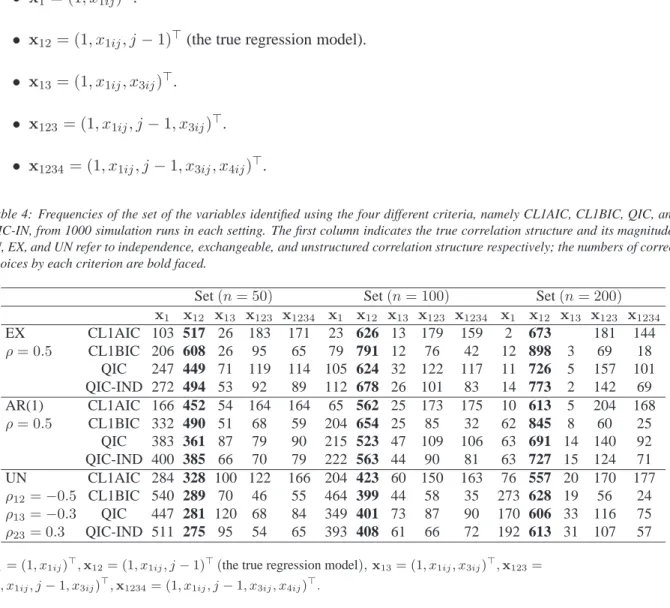
Table 4: Frequencies of the set of the variables identified using the four different criteria, namely CL1AIC, CL1BIC, QIC, and QIC-IN, from 1000 simulation runs in each setting. The first column indicates the true correlation structure and its magnitude; IN, EX, and UN refer to independence, exchangeable, and unstructured correlation structure respectively; the numbers of correct choices by each criterion are bold faced.
Set(n= 50) Set(n= 100) Set(n= 200) x1 x12 x13 x123 x1234 x1 x12 x13 x123 x1234 x1 x12 x13 x123 x1234 EX CL1AIC 103 517 26 183 171 23 626 13 179 159 2 673 181 144 ρ= 0.5 CL1BIC 206 608 26 95 65 79 791 12 76 42 12 898 3 69 18 QIC 247 449 71 119 114 105 624 32 122 117 11 726 5 157 101 QIC-IND 272 494 53 92 89 112 678 26 101 83 14 773 2 142 69 AR(1) CL1AIC 166 452 54 164 164 65 562 25 173 175 10 613 5 204 168 ρ= 0.5 CL1BIC 332 490 51 68 59 204 654 25 85 32 62 845 8 60 25 QIC 383 361 87 79 90 215 523 47 109 106 63 691 14 140 92 QIC-IND 400 385 66 70 79 222 563 44 90 81 63 727 15 124 71 UN CL1AIC 284 328 100 122 166 204 423 60 150 163 76 557 20 170 177 ρ12=−0.5 CL1BIC 540 289 70 46 55 464 399 44 58 35 273 628 19 56 24 ρ13=−0.3 QIC 447 281 120 68 84 349 401 73 87 90 170 606 33 116 75 ρ23= 0.3 QIC-IND 511 275 95 54 65 393 408 61 66 72 192 613 31 107 57 x1= (1, x1ij)⊤,x12= (1, x1ij, j
−1)⊤(the true regression model),x13= (1, x1ij, x3ij)⊤,x123= (1, x1ij, j−1, x3ij)⊤,x1234= (1, x1ij, j−1, x3ij, x4ij)⊤.
In Table4, we present the numbers of times that different subsets of covariates are chosen over 1000 simulation runs under each true correlation structure. Among the criteria, we also use the QIC under independence (QIC-IN), which behaves better than QIC under the true correlation structure [11]. If the true correlation structure is exchangeable or AR(1), CL1BIC performs better than QIC-IN, and its performance improves as the sample size increases. If the true correlation structure is unstructured, CL1AIC and QIC-IN behave similarly; the former behaves better for smaller sample sizes. For all the candidate subsets of covariates, CL1AIC tends to choose the full-model more often than CL1BIC.
5 The Hamilton’s depression data
To select the appropriate correlation structure, we use the proposed model selection criteria in the weighted scores estimating equations, along with the existing model selection criteria in GEE, based on the full model with all covariates and the interaction term between time and treatment (Table5, correlation struc-ture selection).
According to CL1AIC, CL1BIC, and QIC, the optimal correlation structure is the AR(1). CIC, EAIC, and EBIC are not able to reveal that and prefer the independence structure. Furthermore, with the CL1 criteria one can easily distinguish between the various structures, since their difference in magnitude is large. This is not the case for the other criteria, where the differences are rather small. The AR(1) structure is plausible for this example, with measurements that are approximately equally spaced in time, because it forces the correlation between consecutive measurements on a subject to decrease with increasing separa-tion in measurement occasion. For covariate selecsepara-tion, under the preferred AR(1) structure, we fit different models with different subsets of covariates, and find that the full model has the smallest CL1AIC, CL1BIC, and QIC-IND (Table5, variable selection).
Table 5: The values of the different criteria for model selection for the Hamilton’s depression data. The smallest value of each criterion is boldfaced.
Correlation structure selection
Independence Exchangeable AR(1) CL1AIC 10194.88 (1.000) 9832.90 (0.964) 9783.90 (0.960) CL1BIC 10212.42 (1.000) 9866.94 (0.966) 9824.59 (0.962) EAIC 8568.37 (1.000) 8570.30 (1.000) 8570.34 (1.000) EBIC 8582.41 (1.000) 8587.84 (1.001) 8587.89 (1.001) QIC 1511.48 (1.000) 1537.87 (1.017) 1513.56 (1.001) CIC 8.46 (1.000) 8.98 (1.061) 8.41 (0.994) Variable selection Trt Trt+Time Trt×Time CL1AIC-AR(1) 17173.69 (1.000) 9861.18 (0.574) 9783.90 (0.570) CL1BIC-AR(1) 17200.81 (1.000) 9896.32 (0.575) 9824.59 (0.571) QIC-IN 2625.63 (1.000) 1520.67 (0.579) 1511.48 (0.576)
Relative terms of the values of the different criteria for each specific method under consideration are shown in parentheses.
Finally, Table 6 gives the estimates and standard errors of the model parameters obtained using the weighted scores estimating equations and GEE under the optimal AR(1) correlation structure. All esti-mates are similar and consistent. This example also shows that if the correlation structure and the variables in the mean function modelling are correctly specified, then there is no loss in efficiency in GEE.
Table 6: Weighted scores and GEE estimates (Est.), along with their standard errors (SE) under the optimal correlation structure and set of covariates for the Hamilton’s depression data.
Dependence AR(1)
Method GEE Weighted scores Covariates Est. SE Est. SE
Intercept -4.67 0.32 -4.62 0.31 Treatment 0.89 0.40 0.85 0.40 Time 1.17 0.09 1.16 0.08 Treatment×Time -0.36 0.11 -0.34 0.11 ρ 0.44 0.53 0.76 0.03 6 Concluding remarks
In this article, we have introduced binary and Poisson regression in the weighted scores method for re-gression with dependent data. Our method of combining the univariate scores for binary and Poisson regression has the merit of robustness to misspecification of the dependence structure like in generalized
estimating equations, but with the additional advantage, with respect to generalized estimating equations, that dependence is expressed in terms of a “real” multivariate model. We have compared our approach to GEE, and established our method as a viable competitor to GEE methods for both model selection and estimation. The estimated correlation parameters in GEE cannot be interpreted, and sometimes violate the Fr´echet bounds of the feasible range of the correlation [6]. This was the case in the application example as discussed by Sabo and Chaganty [1]. Our working MVN copula model is a proper multivariate model, and the correlations can be interpreted as latent correlations.
Comparing our method with ML, one advantage is that the weight matrices depend on covariances of the scores; that is, only the bivariate marginal probabilities are needed. The ML method for the discretized MVN is feasible, but not easy, because multidimensional integration is needed to compute the MVN rectangle probabilities [21,22]. Also the weighted scores method is in a sense superior compared with the ML method; based on a “working” model leads to unbiased estimating equations if univariate model is correct, while on the other hand ML estimates could be biased if the univariate model is correct but dependence is modelled incorrectly. This is the case in practice since the “true” model is not generally known. So weighted scores is robust to dependence if main interest is in the univariate parameters.
Software
R functions to implement the weighted scores method and the CL1 information criteria for longitudinal binary and count data have been implemented in the package weightedScores [26] within the open source statistical environment R [27].
Acknowledgements
We would like to thank Professor Harry Joe, University of British Columbia, for helpful comments and suggestions and Professor Rao Chaganty, Old Dominion University, for providing the Ham-D data.
Appendix
In what follows we provide technical details for the calculation of the asymptotic covariance matrix for the estimator that solves the CL1 estimating equations, and its form for the case of one dependence parameter
ρ. This is the case for an exchangeable and AR(1) dependence structure, sinceRis(1−ρ)Id+ρOd(Id is the identity matrix of orderdandOdis thed×dmatrix of 1s) and(ρ|j−k|)1≤j,k≤d, respectively.
For positive exchangeable correlation structures, the MVN rectangle probabilities (4) can be quickly computed to a desired accuracy that is 10−6 or less, because thed-dimensional integrals conveniently reduce to 1-dimensional integrals [30, p. 48]. For general correlation structures, there are several papers in the literature, e.g., [31, 32, 33], that focus on the computation of the MVN rectangle probabilities, and, conveniently, the implementation of the proposed algorithms is available in contributed R packages [34,35]. For more details see [21].
Illustrations ford= 4and technical details
Ford = 4 the matrices involved in the calculation of the sensitivity matrix Hg of the composite score
−Hg1 =x⊤i E ∂s(1)i1 (β) ∂νi1 0 0 0 0 ∂s (1) i2 (β) ∂νi2 0 0 0 0 ∂s (1) i3 (β) ∂νi3 0 0 0 0 ∂s (1) i4 (β) ∂νi4 xi; −Hg1,2 =E ∂s(2)i,12(β,ρ12) ∂νi1 ∂s(2)i,12(β,ρ12) ∂νi2 0 0 ∂s(2)i,13(β,ρ13) ∂νi1 0 ∂s(2)i,13(β,ρ13) ∂νi3 0 ∂s(2)i,14(β,ρ14) ∂νi1 0 0 ∂s(2)i,14(β,ρ14) ∂νi4 0 ∂s (2) i,23(β,ρ23) ∂νi2 ∂s(2)i,23(β,ρ23) ∂νi3 0 0 ∂s (2) i,24(β,ρ24) ∂νi2 0 ∂s(2)i,24(β,ρ24) ∂νi4 0 0 ∂s (2) i,34(β,ρ34) ∂νi3 ∂s(2)i,34(β,ρ34) ∂νi4 xi; −Hg2 =E ∂s(2)i,12(β,ρ12) ∂ρ12 0 0 0 0 0 0 ∂s (2) i,13(β,ρ13) ∂ρ13 0 0 0 0 0 0 ∂s (2) i,23(β,ρ14) ∂ρ14 0 0 0 0 0 0 ∂s (2) i,23(β,ρ23) ∂ρ23 0 0 0 0 0 0 ∂s (2) i,24(β,ρ24) ∂ρ24 0 0 0 0 0 0 ∂s (2) i,34(β,ρ34) ∂ρ34 .
The elements of these matrices are calculated as below:
−E∂s (2) i,jk(β, ρjk) ∂ρjk =−E∂ 2ℓ 2(νij, νik, ρjk;yij, yik) ∂ρ2 jk =E ∂ℓ2(νij, νik, ρjk;yij, yik) ∂ρjk 2 , where ∂ℓ2(νij,νik,ρjk;yij,yik) ∂ρjk = ∂f2(yij,yik;νij,νik,ρjk) ∂ρjk /f2(yij, yik;νij, νik, ρjk), −E∂s (2) i,jk(β, ρjk) ∂β = −E∂ 2ℓ 2(νij, νik, ρjk;yij, yik) ∂β∂ρjk = E∂ℓ2(νij, νik, ρjk;yij, yik) ∂β ∂ℓ2(νij, νik, ρjk;yij, yik) ∂ρjk ; ∂ℓ2(νij,νik,ρjk;yij,yik) ∂β = ∂logf2(yij,yik;νij,νik,ρjk) ∂β = ∂f2(yij,yik;νij,νik,ρjk) ∂β /f2(yij, yik;νij, νik, ρjk), ∂f2(yij,yik;νij,νik,ρjk) ∂β = ∂f2(yij,yik;νij,νik,ρjk) ∂νij xij+ ∂f2(yij,yik;νij,νik,ρjk) ∂νik xik, ∂f2(yij,yik;νij,νik,ρjk) ∂νij = ∂f2(yij,yik;νij,νik,ρjk) ∂Φ−1 F1(yij;νij) ∂Φ−1 F 1(yij;νij) ∂νij + ∂f2(yij,yik;νij,νik,ρjk) ∂Φ−1 F1(yij−1;νij) ∂Φ−1 F 1(yij−1;νij) ∂νij , ∂Φ−1 F 1(yij;νij) ∂νij = Pyij 0 ∂f1(yij;νij) ∂νij /φ Φ−1 F 1(yij;νij) , ∂f1(yij;νij) ∂νij =f1(yij;νij) ∂ℓ1(νij;yij) ∂νij . The derivatives ∂f2(yij,yik;νij,νik,ρjk) ∂ρjk and ∂f2(yij,yik;νij,νik,ρjk) ∂Φ−1 F j(yij;νij)
are computed with the R functions exch-mvn.deriv.rho and exchmvn.deriv.margin, respectively, in the R package mprobit [34].
Ford= 4the matrices involved in the calculation of the covariance matrixJg of the composite score
functionsgtake the form:
Ω(1) i = Vars(1) i1 (β) Covs(1) i1 (β),s (1) i2 (β) Covs(1) i1 (β),s (1) i3(β) Covs(1) i1 (β),s (1) i4 (β) Cov s(1) i2(β),s (1) i1 (β) Var s(1) i2 (β) Cov s(1) i2 (β),s (1) i3(β) Cov s(1) i2 (β),s (1) i4 (β) Cov s(1) i3(β),s (1) i1 (β) Cov s(1) i3 (β),s (1) i2 (β) Var s(1) i3 (β) Cov s(1) i3 (β),s (1) i4 (β) Covs(1) i4(β),s (1) i1 (β) Covs(1) i4 (β),s (1) i2 (β) Covs(1) i4 (β),s (1) i3(β) Vars(1) i4 (β) , Ω(1,2) i = Covs(1) i1 ,s (2) i,12 Covs(1) i1 ,s (2) i,13 Covs(1) i1 ,s (2) i,14 Covs(1) i1 ,s (2) i,23 Covs(1) i1 ,s (2) i,24 Covs(1) i1 ,s (2) i,34 Covs(1) i2 ,s (2) i,12 Covs(1) i2 ,s (2) i,13 Covs(1) i2 ,s (2) i,14 Covs(1) i2 ,s (2) i,23 Covs(1) i2 ,s (2) i,24 Covs(1) i2 ,s (2) i,34 Covs(1) i3 ,s (2) i,12 Covs(1) i3 ,s (2) i,13 Covs(1) i3 ,s (2) i,14 Covs(1) i3 ,s (2) i,23 Covs(1) i3 ,s (2) i,24 Covs(1) i3 ,s (2) i,34 Cov s(1) i4 ,s (2) i,12 Cov s(1) i4 ,s (2) i,13 Cov s(1) i4 ,s (2) i,14 Cov s(1) i4 ,s (2) i,23 Cov s(1) i4 ,s (2) i,24 Cov s(1) i4 ,s (2) i,34 , where Covs(1)ij1,s(2)i,j1j2 = X y s(1)ij1s(2)i,j1j2f2(yij1, yij2;νij1, νij2, ρj1j2), Cov s(1)ij 1,s (2) i,j2j3 = X y s(1)ij 1s (2) i,j2j3f3(yij1, yij2, yij3;νij1, νij2, νij3, ρj1j2, ρj1j3, ρj2j3), and Ω(2) i = Var s(2) i,12 Cov s(2) i,12,s (2) i,13 Cov s(2) i,12,s (2) i,14 Cov s(2) i,12,s (2) i,23 Cov s(2) i,12,s (2) i,24 Cov s(2) i,12,s (2) i,34 Cov s(2) i,13,s (2) i,12 Var s(2) i,13 Cov s(2) i,13,s (2) i,14 Cov s(2) i,13,s (2) i,23 Cov s(2) i,13,s (2) i,24 Cov s(2) i,13,s (2) i,34 Covs(2) i,14,s (2) i,12 Covs(2) i,14,s (2) i,13 Vars(2) i,14 Covs(2) i,14,s (2) i,23 Covs(2) i,14,s (2) i,24 Covs(2) i,14,s (2) i,34 Covs(2) i,23,s (2) i,12 Covs(2) i,23,s (2) i,13 Covs(2) i,23,s (2) i,14 Vars(2) i,23 Covs(2) i,23,s (2) i,24 Covs(2) i,23,s (2) i,34 Covs(2) i,24,s (2) i,12 Covs(2) i,24,s (2) i,13 Covs(2) i,24,s (2) i,14 Covs(2) i,24,s (2) i,23 Vars(2) i,24 Covs(2) i,24,s (2) i,34 Cov s(2) i,34,s (2) i,12 Cov s(2) i,34,s (2) i,13 Cov s(2) i,34,s (2) i,14 Cov s(2) i,34,s (2) i,23 Cov s(2) i,34,s (2) i,24 Var s(2) i,34 , where Vars(2)i,j1j2 = X y s(2)i,j1j2s(2)i,j1j2f2(yij1, yij2),
Covs(2)i,j1j2,s(2)i,j1j3 = X
y
s(2)i,j1j2s(2)i,j1j3f3(yij1, yij2, yij3),
Covs(2)i,j1j2,s(2)i,j3j4 = X
y
s(2)i,j1j2s(2)i,j3j4f4(yij1, yij2, yij3, yij4);
the inner sum is taken over all possible vectorsy.
One dependence parameter
DifferentiatingL2with respect toρleads to the bivariate composite score function:
g2 = ∂L2 ∂ρ = n X i=1 s(2)i (β, ρ) =0, wheres(2)i (β, ρ) = P j<k∂ℓ2(νij,νik,ρ;yij,yik) ∂ρ is scalar.
The sensitivity matrixHg of the composite score functionsgis given as below, Hg =−E ∂g ∂θ = −E ∂g1 ∂β −E∂∂g1ρ −E∂g2 ∂β −E∂g2 ∂ρ = H(1) 0 H(2,1) D(2) , whereH(1) = n1Pni x⊤i ∆(1)i xi with ∆(1)i = −E ∂s(1) i (β) ∂νi , H(2,1) = n1 Pni ∆i(2,1)xi with ∆(2i ,1) = −E∂s (2) i (β,ρ) ∂β , andD(2) = n1Pni ∆i(2)with∆(2)i =−E∂s (2) i (β,ρ) ∂ρ , where, −E∂s (2) i (β, ρ) ∂ρ = −E∂ P j<k∂ℓ2(νij, νik, ρ;yij, yik) ∂ρ /∂ρ = −EX j<k ∂2ℓ 2(νij, νik, ρ;yij, yik) ∂ρ2 = X j<k −E∂ 2ℓ 2(νij, νik, ρ;yij, yik) ∂ρ2 = X j<k E(∂ℓ2(νij, νik, ρ;yij, yik) ∂ρ ) 2, and −E∂s (2) i (β, ρ) ∂β = −E∂ P j<k∂ℓ2(νij, νik, ρ;yij, yik) ∂ρ /∂β = −EX j<k ∂2ℓ 2(νij, νik, ρ;yij, yik) ∂ρ∂β = X j<k −E∂ 2ℓ 2(νij, νik, ρ;yij, yik) ∂ρ∂β = X j<k E∂ℓ2(νij, νik, ρ;yij, yik) ∂ρ ∂ℓ2(νij, νik, ρ;yij, yik) ∂β .
The covariance matrixJgof the composite score functionsgis given as below
Jg =Cov(g) = Cov(g1) Cov(g1,g2) Cov(g2,g1) Cov(g2) = J (1) g J(1g,2) J(2g,1) Mg(2) ! =X i x⊤i Ω(1)i xi x⊤i Ω (1,2) i Ω(2i ,1)xi Ω(2)i ! , where Ω(1)i Ω(1i ,2) Ω(2i ,1) Ω(2)i ! = Cov s(1)i (β) Covsi(1)(β),s(2)i (β, ρ) Covs(2)i (β, ρ),si(1)(β) Covs(2)i (β, ρ) ; Covs(1)i (β),s(2)i (β, ρ) = X y s(1)i (β)s(2)i (β, ρ)fd(yi), Covs(2)i (β, ρ),s(2)i (β, ρ) = X y s(2)i (β, ρ)s(2)i (β, ρ)fd(yi).
References
[1] Sabo R, Chaganty NR. What can go wrong when ignoring correlation bounds in the use of generalized estimating equations. Statistics in Medicine 2010; 29:2501–2507.
[2] Liang KY, Zeger SL. Longitudinal data analysis using generalized linear models. Biometrika 1986; 73:13–22. [3] Zeger SL, Liang KY. Longitudinal data analysis for discrete and continuous outcomes. Biometrics 1986; 42:121–130. [4] Halekoh U, Højsgaard S, Yan J. The R package geepack for generalized estimating equations. Journal of Statistical Software
2006; 15:1–11.
[5] Nikoloulopoulos AK, Joe H, Chaganty NR. Weighted scores method for regression models with dependent data. Biostatis-tics 2011; 12:653–665.
[6] Chaganty NR, Joe H. Range of correlation matrices for dependent Bernoulli random variables. Biometrika 2006; 93(1):197– 206.
[7] Albert PS, McShane LM. A generalized estimating equations approach for spatially correlated binary data: Applications to the analysis of neuroimaging data. Biometrics 1995; 51(2):627–638.
[8] Crowder M. On the use of a working correlation matrix in using generalised linear models for repeated measures. Biometrika 1995; 82(2):407–410.
[9] Wang YG, Carey V. Working correlation structure misspecification, estimation and covariate design: Implications for gen-eralised estimating equations performance. Biometrika 2003; 90(1):29–41.
[10] Shults J, Sun W, Tu X, Kim H, Amsterdam J, Hilbe JM, Ten-Have T. A comparison of several approaches for choosing between working correlation structures in generalized estimating equation analysis of longitudinal binary data. Statistics in medicine 2009; 28(18):2338–2355.
[11] Pan W. Akaike’s information criterion in generalized estimating equations. Biometrics 2001; 57:120–125.
[12] Hin LY, Wang YG. Working-correlation-structure identification in generalized estimating equations. Statistics in medicine 2009; 28(4):642–658.
[13] Chen J, Lazar NA. Selection of working correlation structure in generalized estimating equations via empirical likelihood. Journal of Computational and Graphical Statistics 2012; 21(1):18–41.
[14] Varin C, Vidoni P. A note on composite likelihood inference and model selection. Biometrika 2005; 92:519–528.
[15] Gao X, Song PXK. Composite likelihood EM algorithm with applications to multivariate hidden Markov model. Statistica Sinica 2011; 21:165–185.
[16] Zhao Y, Joe H. Composite likelihood estimation in multivariate data analysis. The Canadian Journal of Statistics 2005;
33(3):335–356.
[17] Joe H. Multivariate Models and Dependence Concepts. Chapman & Hall: London, 1997. [18] Ashford JR, Sowden RR. Multivariate probit analysis. Biometrics 1970; 26:535–546.
[19] Muth´en B. Contributions to factor analysis of dichotomous variables. Psychometrika 1978; 43:551–560.
[20] Hausman J, Wise D. A conditional probit model for qualitative choice: Discrete decisions recognizing interdependence and heterogeneous preferences. Econometrica 1978; 45:319–339.
[21] Nikoloulopoulos AK. On the estimation of normal copula discrete regression models using the continuous extension and simulated likelihood. Journal of Statistical Planning and Inference 2013; 143:1923–1937.
[22] Nikoloulopoulos AK. Efficient estimation of high-dimensional multivariate normal copula models with discrete spatial responses. Stochastic Environmental Research and Risk Assessment 2015; DOI:10.1007/s00477-015-1060-2.
[23] Nikoloulopoulos AK, Karlis D. Finite normal mixture copulas for multivariate discrete data modeling. Journal of Statistical Planning and Inference 2009; 139:3878–3890.
[24] Varin C. On composite marginal likelihoods. Advances in Statistical Analysis 2008; 92:1–28.
[25] Varin C, Reid N, Firth D. An overview of composite likelihood methods. Statistica Sinica 2011; 21:5–42.
[26] Nikoloulopoulos AK, Joe H. weightedScores: Weighted scores method for regression models with dependent data 2015. R package version 0.9.5.1.http://CRAN.R-project.org/package=weightedScores.
[27] R Core Team. R: A language and environment for statistical computing 2015. R Foundation for Statistical Computing: Vienna, Austria.http://CRAN.R-project.org/.
[28] Godambe VP. Estimating Functions. Oxford University Press: Oxford, 1991.
[29] Leisch F, Weingessel A, Hornik K. bindata: Generation of Artificial Binary Data 2012. R package version 0.9-19.
http://CRAN.R-project.org/package=bindata.
[30] Johnson NL, Kotz S. Continuous Multivariate Distributions. Wiley: New York, 1972.
[31] Joe H. Approximations to multivariate normal rectangle probabilities based on conditional expectations. Journal of the American Statistical Association 1995; 90(431):957–964.
[32] Genz A. Numerical computation of the multivariate normal probabilities. Journal of Computational and Graphical Statistics 1992; 1:141–150.
[33] Genz A, Bretz F. Methods for the computation of the multivariatet-probabilities. Journal of Computational and Graphical Statistics 2002; 11:950–971.
[34] Joe H, Chou LW, Zhang H. mprobit: Multivariate probit model for binary/ordinal response 2011. R package version 0.9-3.
http://CRAN.R-project.org/package=mprobit.
[35] Genz A, Bretz F, Miwa T, Mi X, Leisch F, Scheipl F, Hothorn T. mvtnorm: Multivariate Normal and t Distributions 2012. R package version 0.9-9992.http://CRAN.R-project.org/package=mvtnorm.