Progressive Multiple Sequence Alignment with Indel Evolution

(1)

Unicentre

CH-1015 Lausanne

http://serval.unil.ch

Year :

2019

Progressive Multiple Sequence Alignment with Indel Evolution

Maiolo Massimo

Maiolo Massimo, 2019, Progressive Multiple Sequence Alignment with Indel Evolution

Originally published at : Thesis, University of Lausanne

Posted at the University of Lausanne Op

Document URN : urn:nbn:ch:serval-BIB_D24577D3A8854

Droits d’auteur

L'Université de Lausanne attire expressément l'attention des utilisateurs sur le fait que tous les

documents publiés dans l'Archive SERVAL sont protégés par le droit d'auteur, conformément à la

loi fédérale sur le droit d'auteur et les droits voisins (LDA). A ce titre, il est indispensable d'obtenir

le consentement préalable de l'auteur et/ou de l’éditeur avant toute utilisation d'une oeuvre ou

d'une partie d'une oeuvre ne relevant pas d'une utilisation à des fins personnelles au sens de la

LDA (art. 19, al. 1 lettre a). A défaut, tout contrevenant s'expose aux sanctions prévues par cette

loi. Nous déclinons toute responsabilité en la matière.

Copyright

The University of Lausanne expressly draws the attention of users to the fact that all documents

published in the SERVAL Archive are protected by copyright in accordance with federal law on

copyright and similar rights (LDA). Accordingly it is indispensable to obtain prior consent from the

author and/or publisher before any use of a work or part of a work for purposes other than

personal use within the meaning of LDA (art. 19, para. 1 letter a). Failure to do so will expose

offenders to the sanctions laid down by this law. We accept no liability in this respect.

(2)

!

Département de biologie computationnelle

Progressive Multiple Sequence Alignment

with Indel Evolution

Thèse de doctorat ès sciences de la vie (PhD)

présentée à la

Faculté de biologie et de médecine

de l’Université de Lausanne

par

Massimo Maiolo

Master of Science SUPSI in Engineering

Jury

Prof. Jérôme Goudet, Président

Prof. Christophe Dessimoz, Directeur de thèse

Prof. Nicolas Salamin, Co-directeur

Dr. Maria Anisimova, Co-directeur

Prof. Olivier Gascuel, expert

Prof. Anna-Sapfo Malaspinas, expert

(3)

(4)

(5)

(6)

©

(7)

(8)

Acknowledgments

“Gratitude is when memory is stored in the heart and not in the

mind.”

– Lional Hampton

The outcomes of this thesis could not have been attained without the many

people who have been involved in my life throughout the years. In different

ways these people have encouraged, mentored, guided, instructed, influenced

and loved me.

Firstly, I have great pleasure in acknowledging my gratitude to Maria

Anisi-mova and Manuel Gil, my PhD advisors, for supporting and assisting me

dur-ing the past four years. I have been fortunate to have been advised by you.

I want to express my gratitude to Lorenzo Gatti who gave me valuable

in-puts in many occasions. We have spent together many many hours coding and

debugging our software package. I am particularly indebted to Simone Ulzega

for helping me a lot especially with the STFT project. He is the colleague that

I have my morning ‘doppio espresso’ with. I would like to express my thanks

to Xiaolei Zhang, our brilliant Master student, for the great collaboration in

the 3D-DP algorithm design. I have appreciated the collaboration with Tiziano

Leidi and Diego Frei, for the impressive experience and for inspirational

dis-cussions with me regarding the code parallelisation.

I am grateful for conversations with Victor Garcia, Spencer Bliven and

Norman Juchler. They have been helpful in giving advises many times during

my time at ZHAW. I’m also glad to have worked with our master students, Ta

Cam Phuong Nguyesan and Jithin Mathew Peechatt.

The members at the Institute of Applied Simulations have contributed to my

professional development, they have been always very kind and friendly as well

as good collaborator. In particular, I am grateful to the administrative

assis-tants Rita Schoepfer Braschler, Simone Frei, Cyril Burkhard and Natyra Ajvazi

at ZHAW along with Susanna Bachmann at UZH, Livia Ioni and Alexandra

Cassoli at UNIL. They kept me organized and were always ready to help.

(9)

vi

ACKNOWLEDGMENTS

I am much obliged also to my former colleagues at SUPSI, I miss Melissa

Gajewsky for the heated discussions and the fun we had together, she has been

a special inspiration to me. I will forever be indebted to my former research

advisor Prof. Andrea Danani, I am very grateful for his scientific advise and

many insightful discussions and suggestions. I still think fondly of my time

spent in his lab. He has been the one letting me pursuing a career in research. I

really enjoyed the time spent with Andrea Bernasconi. The joy and enthusiasm

he has for scientific research was motivational for me. I earnestly thank him

for his influence on my professional life. I am especially thankful to Alberto

Vancheri for the excellent example he has provided as person and admirable

researcher. Alberto was and remains my best role model as scientist, mentor,

and teacher. I never encountered another person so clever and at the same

time so modest. He is extremely knowledgeable in just about everything, that’s

the reason I used to call him ‘Vancher-pedia’.

I especially thank my advisors, Prof. Christian von Mering at the

univer-sity of Zurich and Prof. Christophe Dessimoz at the Univeruniver-sity of Lausanne.

Also, the members of my oral defense committee deserve special thanks, Prof.

Olivier Gascuel, Prof. Anna-Sapfo Malaspinas, Prof. Nicolas Salamin and

Prof. Gerome Goudet. Prof. Andreas Wagner deserve my heartfelt thanks as

being an additional member of my oral exam committee at the University of

Zurich.

I have greatly appreciated also the contributions of time and suggestions of

Prof. Ziheng Yang. I would also like to acknowledge Prof. Marco Comini for

sharing the L

A

TEX template I used for writing this thesis. I acknowledge the

agency that funded my PhD studies. I was financial supported by the Swiss

National Science Foundation.

I would like to express my deepest gratitude to my mom Helen and my dad

Vincenzo. My hard-working parents have sacrificed their lives for my brother,

my sisters and myself. They instilled in me care for and curiosity in the world

around us. It is very sad that my mom left so soon, she would have been proud

of this important achievement. It would be inappropriate if I omit to mention

also my wife’s family, Rosa and Federico, who all have been supportive and

caring.

Nevertheless, the most special thank goes to my wife Teresa and my

daugh-ter Noemi. Definitely, Teresa is the right person for me. All these years,

Teresa has been a true and great supporter. She unconditionally love me

dur-ing my good and bad times. She has faith in me and my intellect, and she

always encouraged me in all possible ways from my Bachelor to my PhD

stud-ies. These past several years have not been an easy ride, both academically,

financially and personally. But she was always at my side. We have both

(10)

learned a lot from each other about life and this experience has strengthened

our relationship. Noemi, my darling little princess, she gave and still gives me

a reason to fight in the most difficult moments. Decisively, she is the light that

brightens my heart. I hope, I can give a better future now that I attained this

important milestone. I love you dearly and thank thoroughly for always

foster-ing me. Your presence was indispensable in a process that is often perceived

as considerably solitaire. My family has always been someone I can count on.

There are no words to convey how deeply I love you.

GOD, I am truly grateful for your exceptional love during this hard but

won-drous journey.

Massimo Maiolo

University of Lausanne

December 2018

(11)

(12)

To my wife

Teresa: for

your

uncondi-

tional love,

end-less support and constant

encourage-ment. You always believed in me and trusted

the decisions I made. You empowered me to

work hard for the things I aspire to achieve.

You are my perfect wife and mother of our

child. To my daughter Noemi: your smile is

the source of my joy and pride. You gave

me the energy I needed for dealing with

all this work. I love you all dearly. You

both are very special and lovely,

the most precious and

valu-able persons in my life. I

am truly thankful

for having

you!

(13)

(14)

Abstract

Here we present, for the first time, a frequentist progressive Multiple Sequence

Alignment (MSA) method based on a rigorous and explicit mathematical

for-mulation of insertions and deletions, namely the Poisson Indel Process (PIP).

Having designed our algorithm in the Maximum Likelihood (ML) framework

has enabled us to avoid the time-consuming Markov Chain Monte Carlo

sam-pling of alignments. Our proposed algorithm aligns two homology paths,

rep-resented by their corresponding MSAs in polynomial time by ML under the

PIP model (Maiolo et al. 2017). The procedure has been integrated into a

pro-gressive procedure that, traversing a given phylogenetic tree, produces at each

internal node the optimal pairwise MSA ending at the root with the alignment

of all the input sequences. The integration of PIP equations into a Dynamic

Programming (DP) approach is not straightforward since the marginal

like-lihood is non-monotonic in the alignment length. Therefore, to account for

the dependence on alignment length we have extended the DP matrices with

a third dimension.

In order to reduce the computational complexity, the algorithm predicts

candidate homologous segments for the purpose of filtering out non-promising

regions in the DP matrix prior to the effective alignment process. Although

our method has been strongly inspired by MAFFT, we have introduced a

number of improvements like for example the use of a multi-scale short-time

Fourier transform (STFT) for the automatic detection of candidate

homolo-gous patterns. Moreover, the use of the multiple-resolution STFT rather than

the Fourier transform improves the detection of homologous regions especially

in the presence of noise and in case of relative short patterns. We have also

defined a more sophisticated and general approach to generate logically sound

paths to connect homologous blocks and resolve overlaps between them.

To mitigate the intrinsic greediness brought by the progressive DP

ap-proach we have also implemented a Stochastic backtracking (Mueckstein et al.

2002) version of the algorithm under the PIP model. In this way, our

pro-gressive algorithm generates at each visited node a distribution of candidate

(15)

sub-optimal alignments. Aligning sub-optimal solutions increases the chances

to escape from local maxima and in our opinion provides a valid strategy to

reduce the progressive bias.

Finally, to account for the among-sites substitution rate variation (ASRV)

we have applied a Gamma distribution to all the rates, insertion and deletion

rates included. However, further analysis are still needed to investigate the

impact of ASRV on the inferred alignments. Our hope is that this feature

could mimic to some extent a long insertion, that is, an insertion of more than

a single character at a time.

The use of a sound mathematical model of indel, namely the Poisson Indel

Process model, is providing more realistic and accurate estimates of MSAs,

phylogenies and model parameters. As a consequence, our new algorithms will

allow not only more accurate phylogeny and alignment inference but it will

also facilitate the estimation of statistical supports of inferred tree partitions

and the ancestral reconstruction of insertions-deletions and substitution

his-tory. Our tool has been developed in a user-friendly software package and is

applicable to large genomic and metagenomic datasets.

(16)

R´

esum´

e

Nous présentons ici, pour la première fois, une méthode d’alignement

progres-sif de séquences multiples (MSA) basée sur une formulation mathématique

rigoureuse et explicite des insertions et des suppressions, à savoir le procédé

Poisson Indel (PIP). Le fait d’avoir conu notre algorithme dans le cadre du

maximum de vraisemblance (ML) nous a permis d’´eviter l’´echantillonnage

fas-tidieux des alignements par la chane de Markov Monte Carlo. L’algorithme

que nous proposons aligne deux trajectoires homologiques, repr´esent´ees par

leurs MSA correspondantes en temps polynomial par ML sous le mod`ele PIP

(Maiolo et al. 2017). La procédure a été intégrée dans une procédure

progres-sive qui, en traversant un arbre phylogénétique donné, produit à chaque noeud

interne le MSA optimal par paires se terminant `a la racine avec l’alignement

de toutes les séquences d’entrée. L’intégration des équations PIP dans une

ap-proche de programmation dynamique (DP) n’est pas simple puisque la

prob-abilit´e marginale est non monotone dans la longueur de l’alignement. Par

conséquent, pour tenir compte de la dépendance à la longueur d’alignement,

nous avons ´etendu les matrices DP avec une troisi`eme dimension.

Afin de réduire la complexité des calculs, l’algorithme prédit les segments

homologues candidats afin de filtrer les r´egions non prometteuses dans la

ma-trice DP avant le processus d’alignement efficace. Bien que notre m´ethode

soit fortement inspir´ee du MAFFT, nous avons introduit un certain

nom-bre d’am´eliorations comme par exemple l’utilisation d’une transform´ee de

Fourier multi-échelle de courte durée (STFT) pour la détection automatique

des mod`eles homologues candidats. De plus, l’utilisation de la STFT

mul-tirésolution plutt que de la transformée de Fourier améliore la détection des

r´egions homologues, en particulier en pr´esence de bruit et dans le cas de

mo-tifs relativement courts. Nous avons ´egalement d´efini une approche plus

so-phistiquée et plus générale pour générer des chemins logiquement sains pour

connecter des blocs homologues et r´esoudre les chevauchements entre eux.

Pour atténuer l’avidité intrinsèque apportée par l’approche progressive de

la PD, nous avons ´egalement mis en uvre une version r´etrospective

(17)

stochas-tique (Mueckstein et al. 2002) de l’algorithme selon le mod`ele PIP. De cette

faon, notre algorithme progressif génère à chaque nud visité une distribution

des alignements optimaux candidats. L’alignement de solutions

sous-optimales augmente les chances d’´echapper aux maxima locaux et, `a notre

avis, fournit une strat´egie valable pour r´eduire le biais progressif.

Enfin, pour tenir compte de la variation du taux de substitution entre les

sites (ASRV), nous avons appliqu´e une distribution gamma `a tous les taux,

taux d’insertion et de suppression inclus. Toutefois, une analyse plus

appro-fondie est encore nécessaire pour étudier l’impact de l’ASRV sur les tracés

déduits. Nous espérons que cette caractéristique pourrait imiter dans une

cer-taine mesure une insertion ” longue ”, c’est- `a-dire une insertion de plus d’un

caract`ere `a la fois.

L’utilisation d’un modèle mathématique solide de l’indel, à savoir le modèle

du processus de Poisson Indel, fournit des estimations plus r´ealistes et plus

précises des ASM, des phylogénies et des paramètres du modèle. Par conséquent,

nos nouveaux algorithmes permettront non seulement une phylog´enie et une

inférence d’alignement plus précises, mais ils faciliteront également l’estimation

des supports statistiques des partitions d’arbres inf´er´ees et la reconstruction

ancestrale des insertions-suppressions et de l’historique des substitutions. Notre

outil a été développé dans un progiciel convivial et est applicable aux grands

ensembles de données génomiques et métagénomiques.

(18)

Contents

List of Symbols

xxvii

List of Acronyms

xxxv

Introduction

xxxvii

Main result of the thesis

lv

Outline

lvii

I

Progressive Multiple Sequence Alignment with

In-del Evolution

1

1 Progressive Dynamic Programming under PIP model

3

1.1

Introduction

. . . .

3

1.2

Likelihood computation of a column

p

(

c

)

. . . .

5

1.3

Likelihood computation of a column

p

(

c

∅)

. . . .

7

2 3D Dynamic Programming under PIP

11

2.1

Introduction

. . . 11

2.2

Alignment at node

v

3

. . . 14

2.3

Alignment at node

v

5

. . . 20

2.4

Alignment at node Ω

. . . 24

2.5

Tracebacking

. . . 25

2.6

Early stop condition

. . . 27

3 Stochastic backtracking DP algorithm

29

3.1

Introduction

. . . 29

3.2

Partition functions

. . . 30

3.3

The partition functions

Z

M

,

Z

X

and

Z

Y

. . . 31

3.4

Forward recursion

. . . 33

3.5

Backward recursion

. . . 38

(19)

xvi

Contents

4 Marginal Likelihood with Rate Variation Across Sites

49

4.1

Introduction

. . . 49

4.2

PIP equations under ASRV

. . . 51

5 Multi-scale STFT based homologous blocks detection

55

5.1

Introduction

. . . 55

5.2

Fourier transform

. . . 58

5.3

Short-time Fourier transform

. . . 59

5.3.1

The Heisenberg Uncertainty Principle

. . . 62

5.4

Algorithm overview

. . . 63

5.4.1

Sequence residues to signal conversion

. . . 68

5.4.2

Signal padding

. . . 70

5.4.3

Fourier transform based homology detection

. . . 71

5.4.4

Multi-scale STFT based homology detection

. . . 73

5.4.5

Homology matrix and optimal path

. . . 83

5.4.6

Final alignment

. . . 91

5.5

STFT vs. FT approach for block detection

. . . 93

5.5.1

Noise sensitivity

. . . 93

5.5.2

Pattern length sensitivity

. . . 94

6 Progressive bias analysis

97

6.1

Introduction

. . . 97

6.2

Alignment with unbalanced tree

. . . 99

6.2.1

Global alignment

. . . 99

6.2.2

Progressive alignment

. . . 101

6.2.3

Progressive bias with unbalanced tree

. . . 102

6.3

Alignment with balanced tree

. . . 104

6.3.1

Global alignment

. . . 104

6.3.2

Progressive alignment

. . . 104

Discussion & Conclusions

107

II

Appendices

113

A Some technicalities

115

A.1 Detailed derivation of the marginal likelihood function

ϕ

(

v

)

. . . 115

A.2 Detailed derivation of the survival probability function

β

(

v

)

. . 120

(20)

Contents

xvii

B Reversibility of TKF91 and PIP

125

B.1 Introduction to TKF91

. . . 125

B.2 Time-reversible evolutionary process

. . . 128

B.3 Reversibility of TKF91

. . . 129

B.4 Reversibility of PIP

. . . 133

C Characterization of Indel rates

137

C.1 Introduction

. . . 137

C.2 lnferring indel rates from a given MSA

. . . 139

D Doob-Gillespie method and PIP description

145

D.1 Doob-Gillespie method

. . . 145

D.1.1 When does the next event happen?

. . . 146

D.1.2 What kind of event happens next?

. . . 148

D.2 Local PIP description

. . . 148

E Grantham’s distance

151

E.1 Introduction

. . . 151

E.2 Grantham’s distance computation

. . . 152

F Homologous blocks overlap resolution

159

G Multiple sequence alignment evaluation

165

G.1 Overview

. . . 165

G.2 Benchmarks

. . . 167

Bibliography

173

III

Journal article

189

Progressive multiple sequence alignment with indel evolution

. . . 191

(21)

(22)

List of Figures

1

Tree of life.

. . . xxxviii

2

Genetic variations at the molecular level.

. . . .

xl

3

DNA, RNA and protein synthesis.

. . . xlii

4

MSA and corresponding homology paths.

. . . xlv

5

Progressive Dynamic Programming.

. . . xlviii

1.1

Rooted topology used to illustrate the PIP-DP formulation.

. .

4

2.1

Phylogenetic tree

τ

.

. . . 12

2.2

Four three-dimensional sparse DP matrices.

. . . 12

2.3

An example of

ϕ

(

|

m

|

).

. . . 13

2.4

Cells computed at layer

m

= 0.

. . . 14

2.5

Homology paths at layer

m

= 0.

. . . 16

2.6

Cells computed layer

m

= 1.

. . . 17

2.7

Homology path representing a match.

. . . 18

2.8

Homologous scenarios at the node

v

3. 1.

. . . 19

2.9

Homologous scenarios at the node

v

3

. 2.

. . . 19

2.10 Cells computed at layer

m

= 2.

. . . 21

2.11 Homology paths at node

v

5. 1.

. . . 22

v

5. 2.

. . . 23

v

5

. 3.

. . . 24

2.14 Homology paths at node

v

5. 4.

. . . 24

2.15 Homology paths at the root Ω.

. . . 25

2.16 Possible starting points of the traceback phase.

. . . 26

2.17 Cells with likelihood different from 0.

. . . 27

2.18 Likelihood values of the last column.

. . . 28

3.1

Six partition functions.

. . . 33

3.2

Paths connected to

P

M

(3

,

3

,

4).

. . . 34

3.3

Cell dependencies in the 3D-DP matrices.

. . . 34

3.4

Possible homologous paths at

Z

M

(3

,

3

,

4).

. . . 37

3.5

Possible homologous paths at

Z

X

(3

,

3

,

4).

. . . 38

3.6

Possible homologous paths at

Z

Y

(3

,

3

,

4).

. . . 39

3.7

Last column in the 3D-DP matrices.

. . . 40

(23)

xx

List of Figures

3.9

Probability distortion as function of the temperature.

. . . 44

3.10 Probability distortion at

T

= 0

.

1.

. . . 45

T

= 0

.

3.

. . . 45

T

= 10.

. . . 46

3.13 Stochastic backtracking paths at different temperatures.

. . . . 47

4.1

Gamma probability distribution functions.

. . . 51

5.1

Theoretical speed-up as function of the number of blocks.

. . . . 57

5.2

Windowed signal.

. . . 60

5.3

Tiling of the time-frequency space.

. . . 63

5.4

FT coefficients

f

k

.

. . . 65

5.5

Column-gap content.

. . . 66

5.6

Overlapping and non-overlapping blocks.

. . . 67

5.7

Padding scheme with

S

w

= 64.

. . . 71

5.8

Padding scheme with

S

w

= 32.

. . . 71

5.9

Window functions examples.

. . . 74

5.10 Boundaries effects at different resolution scales.

. . . 75

5.11 STFT spectrogram.

. . . 76

5.12 First analysis at two different window size.

. . . 77

5.13 Window functions at different resolution level.

. . . 78

5.14 Spectrogram slice at different sliding length.

. . . 79

5.15 Noise threshold convergence.

. . . 80

5.16 Multi-scale STFT surfaces.

. . . 81

5.17 Blocks boundaries analyzed at different scales.

. . . 82

5.18 Multi-resolution boundary detection.

. . . 84

5.19 Example of overlapping blocks.

. . . 85

5.20 Tree of blocks representing possible paths.

. . . 86

5.21 Example of overlapping blocks and their resolution. i).

. . . 87

5.22 Example of overlapping blocks and their resolution. ii).

. . . 87

5.23 Example of overlapping blocks and their resolution. iii).

. . . 88

5.24 Example of overlapping blocks and their resolution. iv).

. . . 88

5.25 Overlap-free paths.

. . . 89

5.26 Homologous and linking blocks.

. . . 90

5.27 Magnification of connecting corner.

. . . 90

5.28 Homologous and linking blocks and magnification.

. . . 90

5.29 MSA obtained with/without STFT.

. . . 92

5.30 Noisy pattern experiment.

. . . 93

5.31 Noise sensitivity.

. . . 94

(24)

List of Figures

xxi

5.33 Pattern length.

. . . 95

6.1

Topologies used to quantify the progressive bias.

. . . 98

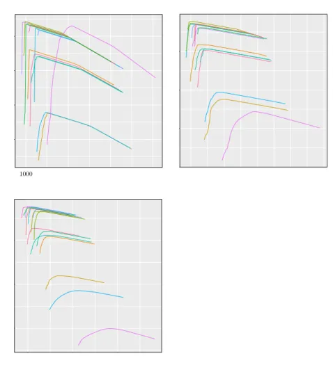
6.2

Marginal likelihood curves at the root node Ω.

. . . 101

6.3

Marginal likelihood curves at the root node

v

2.

. . . 103

6.4

Marginal likelihood curves at the root node

v

1.

. . . 103

6.5

Marginal likelihood curves at node

v

1.

. . . 105

6.6

Marginal likelihood curves at the root Ω.

. . . 106

6.7

Progressive bias analysis.

. . . 106

A.1 Graphical representation of

U

and

W

.

. . . 120

B.1 Time reversibility.

. . . 129

B.2 Four pairwise alignments.

. . . 131

B.3 Two pairwise alignments.

. . . 132

B.4 Topology used to test the reversibility of PIP.

. . . 133

B.5 Representation of likelihood under PIP.

. . . 135

C.1 Possible fate of characters.

. . . 138

C.2 Number of characters through time.

. . . 140

C.3

n

H,

n

G

and

n

H

+

n

G

as function of

I

. . . 142

C.4

n

H,

n

G

and

n

H

+

n

G

as function of

τ

. . . 142

C.5

n

H,

n

G

and

n

H

+

n

G

as function of

λ

. . . 143

C.6

n

H,

n

G

and

n

H

+

n

G

as function of

µ

. . . 143

D.1 Doob-Gillespie method under PIP. Step 1.

. . . 150

E.1 Standardized and non standardized volumes.

. . . 153

E.2 Cross-correlation vs. Grantham’s distance approach.

. . . 154

E.3 Grantham’s distance coefficients.

. . . 157

F.1 Overlaps table.

. . . 163

G.1 BALiBASE benchmark dataset RV911-115: phylogenetic tree.

. 168

G.2 Evolutionary vs Structural alignment. Columns (1-200).

. . . . 168

. . . 169

. . . 170

(25)

xxii

List of Figures

. . 171

(26)

List of Tables

5.1 Amino-acids physiochemical properties.

. . . 69

6.1 MSAs potentially be generated at node

v

1.

. . . 99

6.2 MSAs potentially be generated at node

v

2.

. . . 99

6.3 MSAs potentially be generated at the root Ω.

. . . 100

(27)

(28)

List of Algorithms

1

Doob-Gillespie-PIP procedure

. . . 149

2

Overlap resolution procedure

. . . 160

3

Create block tree procedure

. . . 160

4

Expand node procedure

. . . 161

5

Resolve all overlaps procedure

. . . 161

6

Resolve single path procedure

. . . 161

7

Resolve pairs procedure

. . . 162

8

Resolve overlap pairs procedure

. . . 162

(29)

(30)

List of Symbols

H

(

v

) denotes an homology path of a single character generated by a

substi-tution-deletion continuous-time Markov Chain process along a the

phy-logeny. 123

L ρ

(

v

j

, v

k

)

length of the path that connects

v

j

to

v

k

. Corresponds to the sum

of branch length

b

(

v

) for all the edges connecting the two end points (

v

j

and

v

k

). 3

Γ symbol for the gamma distribution function. The density probability

func-tion is defined as

f

(

x

) =

θ

k

Γ(k)

1

x

k

−

1

e

−

x

θ

=

β

α

Γ(α)

x

α

−

1

e

−

βx

with (

k, θ

) and

(

α, β

) positive numbers. 51

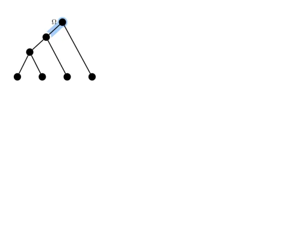
Ω phylogenetic tree root. The root represents the most recent common

ances-tor of all of the taxa in the tree. 52–54, 123

S

M

sparse 3-dimensional Dynamic Programming matrix. It contains the

like-lihood values for

match

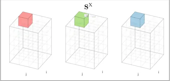
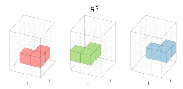
state. xxvii, 14, 16, 18, 27

S

M,X,Y

short notation for

S

M

,

S

X

and

S

Y

. 16, 18, 21, 26–28

S

T

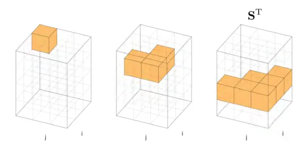
sparse 3-dimensional Dynamic Programming traceback matrix. It stores at

each position (

i, j, k

) which matrix contains the highest likelihood value.

By convention the index 1 stands for

S

M

, 2 for

S

X

and 3 for

S

Y

. 14,

25–27

S

X

sparse 3-dimensional Dynamic Programming matrix. It contains the

gapX

state. xxvii, 14, 16, 23, 27

S

Y

sparse 3-dimensional Dynamic Programming matrix. It contains the

gapY

state. xxvii, 14, 16, 27

k

ν

k

normalizing measure for the Poisson process. It corresponds to

k

ν

k

=

λ

k

τ

k

+

λ

µ

. 17, 18, 20, 116, 139, 140

k

τ

k

tree length obtained summing up all the branch lengths

b

(

v

) for

v

∈ V

.

xxxiii, 6, 18, 52, 116, 133, 134, 138–141

(31)

xxviii

List of Symbols

α

(

v

) corresponds to the sum of all the prior insertion probabilities

ι

(

v

) and

survival probabilities

β

(

v

) from the root to a particular node

v

on the

path

ρ

(

v,

Ω). It follows that for

v

∈ V

:

α

(

v

) =

k

τ

k

1/µ

+1/µ

. 7

∗

hadamard product between two arrays. The hadamard product between two

arrays

x

and

y

of same size corresponds to (

x

∗

y

)(

i

) =

x

(

i

)

·

y

(

i

). 5, 17,

22, 23, 133

β

(

v

) survival probability associated to the node

v

given an insertion, on a

random location, on the edge (pa

→

v

) of length

b

(

v

). See Appendix

A.2

for its detailed derivation.. xxviii, 4, 120, 123

π

extended steady state frequencies. It is represented as an array of size

|A

|×

1 obtained as the quasi-stationary distribution of

Q

.

π

(

i

) contains the

background frequency of the character at the position

i

in the extended

alphabet

A

. The steady state probability of a gap is always 0. See also

π

. 17, 133–135, 150

π

steady state frequencies. For instance using a nucleotide alphabet, the

stationary frequencies,

π

A

,

π

C

,

π

G

,

π

T

correspond to equilibrium base

compositions of the four states. The background frequencies are stored

into an array of size

|A| ×

1 and computed as the limiting distribution

when

t

→ ∞

, that is

π

exp(

Q

t

) =

π

. xxviii

◦

dot product between two arrays. The scalar (dot) product between two

arrays

x

and

y

of same size corresponds to

x

◦

y

=

P

i

x

(

i

)

·

y

(

i

). 5, 15,

17, 20–24, 52, 54, 133

δ

Ω

(d

t

) (continuous) dirac function defined on the topology. It returns 1 at the

root node and 0 elsewhere. 150

it means ‘putatively homologue to’. Hence, A

i

B

j

means that A

i

is

(puta-tively) homologue to B

j

. 16, 18, 19, 22, 31, 32, 36, 85

it denotes a gap state which is an absorbing state in the Markov chain under

the PIP model. It means that once the system enters in gap state it

cannot change anymore, or in other words, a gap never gives birth to

any character. 15, 123

η

(

v

) recursive formula associated to the node

v

that computes the character

deletion probability on the sub-tree rooted at node

v

. 8

(32)

List of Symbols

xxix

ι

(

v

) prior probability of a single character insertion on the branch associated

to

v

with

P

v

∈V

ι

(

v

) = 1. The prior insertion probability of a character

along the edge belonging to

v

∈ V \

Ω is proportional to its length

b

(

v

).

xxviii

λ

single character insertion rate.

λ

is kept constant during the entire

evolutio-nary process (static or time-invariant parameter) and does not depend

on the particular character inserted. 116, 138–141

E

denotes the expectation function. 50, 51, 115

P

symbol for the probability function. 126

Q

extended substitution rate matrix with an extra column and an extra row

to account for the gap character (absorbing state

). With the extended

alphabet of nucleotide for instance

Q

has dimension of 5

×

5. See also

Q

. 52, 123

Q

infinitesimal generator matrix completely describing the Markov process.

Q

contains the rates a continuous time Markov chain moves between states.

Therefore

Q

i,j

is the rate at which character

i

mutates into character

j

.

By using the nucleotide for instance

Q

is a matrix of size 4

×

4. xxix

X

set of input sequences. A sequence is a string of characters belonging to a

given alphabet

A

. Typically there are three kind of standard alphabets:

nucleotides, amino-acids or codons alphabet. 115

Z

M,X,Y

short notation for

Z

M

,

Z

X

and

Z

Y

. 33, 36, 38, 41, 43

Z

M

sparse 3-dimensional dynamic matrix containing the partition function of

alignments ending in state

match

. 31, 32, 35, 36, 40

Z

X

alignments ending in state

gapX

. 31, 32, 36, 37

Z

Y

alignments ending in state

gapY

. 31, 32, 36, 37

Z

total partition function obtained summing up

Z

M

,

Z

X

and

Z

Y

. 35

A

extended alphabet. It is defined as

A

=

A ∪

where

is an absorbing

state (gap character). Under PIP a gap is considered as an extra state

added to the canonical ones. See also

A

. xxviii, xxxii, liii, 5, 123

(33)

xxx

List of Symbols

A

represents the alphabet. A sequence is commonly represented as a string of

characters belonging to a given alphabet. The three alphabets commonly

used are of type

nucleotides

,

amino-acids

or

codons

. For instance the

nucleotide alphabet contains the four letters

{

A, T, G, C

}

. xxix, xxxi,

liii, 3, 123, 133

B

set of candidate homologous blocks detected by the Fourier Transform or the

short-time Fourier Transform. Blocks are then aligned as independent

DP sub-problems.. 83, 159

E

set of edges. An edge is a link connecting

v

with pa(

v

) and has associated

a length indicated as

b

(

e

) =

b

(

v

). xxxi, xxxiii

I

set of vertices

I ∪V

where an insertion could have happened. It corresponds

to the set of vertices having a felsenstein’s weight different from 0. liv,

52, 123

L

set of leaves where

L ⊂ V

. Leaves are nodes without children. The input

sequences are associated at the leaves before aligning them for instance

with a progressive DP procedure. 8, 52, 123

P

set of candidate paths between candidate homologous blocks. Prior to

in-dependently align the single blocks an algorithm has to connect logically,

all the blocks belonging to a path

P

that respect the order of the columns

and avoid any duplication.. xxxii, 83, 86, 159, 160

T

nth tree that represents all possible paths connecting in a meaningful way

the detected homologous blocks.. 83

U

(0

, t

) uniform (continuous) distribution on the interval (0

, t

), with

t >

0. 120

V

finite subset of vertices (branching points in the topology) where

V ⊂

τ

, in

fact under PIP the topology is considered as a continuous set of points.

52, 54, 116, 123

W

(

µ

) exponential distribution with parameter

µ

, describes for instance the

(waiting) time between consecutive events in a Poisson point process.

120

W

L

denotes the Lambert-W function. The Lambert-W function is a set of

functions (branches) of the function

f

(

z

) =

z

exp(

z

) where

z

is a complex

number, therefore

z

=

f

−

1

(

z

exp(

z

)) =

W

L

(

z

exp(

z

))

.

For any complex

number

z

0

=

z

exp(

z

) we get

z

0

=

W

L

(

z

0

) exp

W

L

(

z

0

)

(34)

List of Symbols

xxxi

1

indicator function. The indicator function returns the value 1 if the function

argument is true, 0 otherwise. liv, 3–5, 52

−

character symbol for the gap character, its state is denoted with the simbol

. 15

Poi stands for Poisson probability/distribution. 137, 138, 150

child(

v

) child node of

v

, the next node (below), directed linked to

v

. The

topologies considered here are always binary trees, it follows that each

internal node

v

∈ V \

Ω has degree 3 (2 children). The root Ω has

degree 2 (no parent node) and leaves do not have any children (degree

1). Accordingly, pa(child(

v

)) =

v

for

v

∈ V \

Ω. xxxi

pa(

v

) parent node of

v

, the next node (above), directed linked to

v

. Only the

root Ω does not have any parent node. It follows that child(pa(

v

)) =

v

for

v

∈ V \

Ω (see also child(

v

)). 3, 4

µ

single character deletion rate.

µ

is kept constant during the entire

evolutio-nary process (static or time-invariant parameter) and does not depend

on the particular character deleted. 116, 120, 121, 126, 130, 132, 140,

141

ν

(d

t

) Poisson process intensity defined on the topology, the latter considered

a continuous set of point. Under PIP this intensity is defines as

ν

(d

t

) =

λ

·

τ

(d

t

) +

µ

1

·

δ

Ω

(d

t

)

. 150

ρ

(

v

j

, v

k

) it denotes the set of nodes in the path

v

j

to

v

k

where

v

j

, v

k

∈ V

.

A path is a connected sequence of edges

e

∈ E

and is defined on the

topology. 3

\

the set difference operator. It is defined as

A

\

B

=

{

x

:

x

∈

A

and

x /

∈

B

}

.

27, 52–54, 123

σ

represent a character from the set of characters of a given alphabet

A

or

A

. 123

τ

(d

t

) Lebesgue measure on the topology. Its value corresponds to the distance

measured from a given point to the root. 150

τ

phylogenetic tree. Under PIP the phylogeny

τ

is a continuous set of points,

its topology is denoted by (

L

,

E

), where

V ⊂

τ

is equal to the finite

subset of vertices (branching points), the leaves

L ⊂ V

and the root Ω,

and where

E

is the set of edges. 11, 51, 115, 138, 141

(35)

xxxii

List of Symbols

θ

is the collection of model parameters (branch lengths, substitution rate

ma-trix, insertion/deletion rate, . . . ). 126, 127, 130

ϕ p

(

c

∅

)

,

|

m

|

marginal likelihood of non-observable empty columns for an

a-lignment of length

|

m

|

where

p

(

c

∅

) is the likelihood of a single MSA

column full of gaps. See Appendix

A.1

for its detailed derivation. 53,

115, 116

|A

|

cardinality (number of elements) of the (extended) alphabet

A

. For the

nucleotide alphabet, for instance,

|A

|

= 5. See also

A

. 5

|B|

cardinality of the set

B

which corresponds to the total number of

homol-ogous blocks detected by the Fourier Transform or short-time Fourier

Transform. 83

|

m

|

number of (observed) columns in an alignment

m

. An alignment

m

con-tains

n

columns, where

|

m

|

are observable and

n

− |

m

|

are full of gaps

and hence in general are not represented in an alignment. 13, 14, 17, 21,

51, 115–117, 140

b

Z

M

alignments starting in state

match

and ending once all the characters

have been inserted into the alignment. 31

b

Z

X

alignments starting in state

gapX

have been inserted into the alignment. 31

b

Z

Y

alignments starting in state

gapY

have been inserted into the alignment. 31

e

P

set of overlap-free paths. See Appendix

F

for a description of the algorithm

that resolve the block overlap for a path

p

∈ P

. 87, 160

ξ

(

v

) it represents the non-survival probability associated to the node

v

ob-tained as

ξ

(

v

) = 1

−

ζ

(

v

) which corresponds therefore at the

complemen-tary probability to the survival probability

ζ

. 4

ζ

(

v

) ‘pure’ survival probability associated to the node

v

given an insertion,

on a random location, on the path (pa

→

Ω). Differently from the

function

β

(

v

) the character is already present at pa(

v

) whereas in

β

(

v

)

the character is inserted on a random location along the edge belonging

to

v

. 3, 4

(36)

List of Symbols

xxxiii

b

(

v

) branch length associated to node

v

, which is the length of the edge from

pa(

v

) to

v

. 123

c

∅

MSA column containing only gap characters. Such columns are not

observ-able in an MSA and the number thereof is unknown. xxxiii, 9, 13–15,

18, 21, 39, 51, 53, 115, 123

e

it denotes an edge with

e

∈ E

between

v

and pa(

v

) with

b

(

e

) =

b

(

v

). 3, 120,

121

f

v

felsenstein’s weight. It corresponds to the likelihood under the given

topol-ogy of a given MSA column accounting for the process of substitution

and deletion. See Appendix

A.3

for more details. 123

n

G

number of columns containing gaps (but not full of gaps), corresponds to

n

G

=

λ

· k

τ

k

+

λ

µ

h

1

−

exp(

−k

τ

k

µ

)

i

. See Appendix

C

for more details.

141

n

H

number of columns without gaps, where

n

H

=

λ

µ

exp(

−k

τ

k

µ

). See

Ap-pendix

C

for more details. 141

p

τ

(

m

) marginal likelihood function under PIP of an alignment

m

given a

phy-logenetic tree

τ

, marginalized over ancestral states (see the original paper

for more details [

13

]). 115

p

v

(

c

∅

) likelihood of an MSA column full of gaps computed rooting the topology

at node

v

. When omitted,

v

= Ω. 9

(37)

(38)

List of Acronyms

ASRV

Across Sites Rate Variation. lii, 11, 49

CDF

cumulative distribution function. 146

CTMC

Continuous-Time Markov Chains. 125, 149

DP

Dynamic Programming. xlvii, 11, 23, 29, 33, 46, 56

FFT

Fast Fourier Transform. 56, 57, 64, 68, 151

indel

stands for insertions and/or deletions. xli, 140

ML

Maximum Likelihood. 56

MSA

Multiple Sequence Alignment. xliv, xlvi, 29

PDF

probability distribution function. 51, 121, 147

PIP

Poisson Indel Process (see [

13

]). 31, 146

SB

Stochastic Backtracking. 30, 31, 34, 36–39, 44–46

SP

sum-of-pairs. xlvi, xlvii, 165

(39)

(40)

Introduction

“We are at the very beginning of time for the human race. It is not

unreasonable that we grapple with problems. But there are tens of

thousands of years in the future. Our responsibility is to do what we

can, learn what we can, improve the solutions, and pass them on.”

– Richard P. Feynman

E

volution

is the genetic code alteration of a population over

time mainly driven by natural selection. The modern theory

of evolution is supported with evidences by many scientific

do-mains, not only from biological sciences but also, to mention

a few, from geology, anthropology, chemistry, physics,

math-ematics, astrophysics, psychology as well as behavioral and

social sciences. In 1859,

Charles Darwin

published the seminal book

On the

Origin of Species

where he elaborated the scientific theory of evolution by

nat-ural selection. Since then, many other discoveries in the life sciences endorsed

or extended his hypothesis, that is, all organisms are to some extent related,

species evolve as response to natural selection. To quote

Theodosius

Dobzhan-sky

, a prominent Ukrainian-American geneticist and evolutionary biologist,

“

Nothing in biology makes sense except in the light of evolution

”.

Nonetheless, natural selection is not the single evolutionary driving force for

the biodiversity, variations occur for example also via mutations, sexual

se-lection, genetic drift, and artificial selection. However, selection can occur

only if traits exhibits some genetic variability within a population. Although

evolution happens at the level of population rather than at the single

individ-ual level, heritable changes take place in individindivid-uals and those bringing any

phenotypic advantage are more likely to be passed at the next generations.

Therefore, the frequency of advantageous alleles increases with the time while

that of disadvantageous ones tends to diminish. These individual phenotypic

changes within a population are modifying the distribution of phenotypic

val-ues over time. When the phenotypic shift brings some benefit to the fitness,

than it is likely that this modification is conserved over generations.

(41)

xxxviii

Introduction

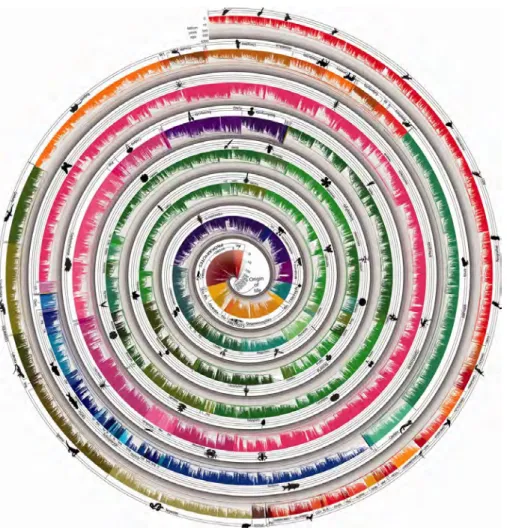
Figure 1: Tree of life reveals clock-like speciation and diversification. A timetree

of 50,632 species synthesized from times of divergence published in 2,274 studies.

Evolutionary history is compressed into a narrow strip and then arranged in a spiral

with one end in the middle and the other on the outside. Therefore, time progresses

across the width of the strip at all places, rather than along the spiral. Time is shown

in billions of years on a log scale and indicated throughout by bands of gray. Major

taxonomic groups are labeled and the different color ranges correspond to the main

taxonomic divisions of our tree.

Image and caption reproduced with permission from Blair Hedges et al. [

51

].

Along with natural selection processes, also catastrophic events or

environ-mental changes may induce changes in the gene pools of a population. This

population gene diversity is actually crucial to survive within a dynamically

changing environment. A wide assortment of genes increases the probability

that some individuals possess the differentiated allele needed to better adapt

(42)

Introduction

xxxix

to the environment. In small population sizes the genetic variability in general

decreases as the inbreeding or the mating between individuals having similar

genetic makeup is more likely to occur. Less biodiversity implies, in turn, less

chances of coping with environmental variability.

Genetic variation increases with the spontaneous generation of new alleles

but also because of gene flowing (horizontal/lateral gene transfer) from other

individuals which introduce in this way new traits from foreign populations.

These phenomena along with natural selection, establish part of the natural

process yielding towards evolution and speciation. Indeed, life continues to

evolve through speciations and extinctions, two key mechanisms controlling

biodiversity. These events are depicted graphically be means of phylogenetic

trees. An example is provided in Figure

1

.

However, speciation and extinction are events happening at different rates.

Speciation and extinction rates establish the frequency at which new species

originate and are lost over evolutionary time. Typically, species that promote

speciation are also highly specialized to a particular environment, are often

isolated or have a low population size. The same characteristics are associated

also with extinction. Actually, specialized species are susceptible to

environ-mental change and therefore are predisposed to disappear rapidly. Speciation

can occur slowly and gradually often described by point mutations or appear

with silent periods interrupted by event “bursts”. As a result, when two

pop-ulations that have diverged from a common ancestor become reproductively

distincts, i.e. capable of interbreeding and exchanging genetic information to

produce fertile offspring, a new species arise.

The carriers of the genetic information are DNA and RNA, they constitute

the building elements of any genetic code and of different pathways. These

“building blocks” are conserved across all the species while the encoded

infor-mation may changes. Observing the conserved core processes and the essential

features shared among all organisms, both extinct or extant, suggests that all

organisms descent from a common ancestry (see Figure

1

). In fact, some of

these mechanisms are so sophisticated that the probability that they emerged

independently several times is almost negligible. All living beings endowing

these features, and from which diversification occurred, led to the development

of the three domains: Archaea, Bacteria, and Eucarya. The universal common

ancestor had as its genetic material the DNA which, through transcription and

translation, expressed its genetic code. Phylogenetic trees show graphically the

evolutionary history of acquired and lost traits during the evolution.

(43)

xl

Introduction

substitution

<latexit sha1_base64="EHTcu7lVtu0tS3V33CeHFezbMlE=">AAAB/HicbVDLSgMxFM3UV62v0S7dBIvgqsyIoMuiG5cV7APaoWTSTBuayQzJjViG+ituXCji1g9x59+YaWehrQcCh3Pu4d6cMBVcg+d9O6W19Y3NrfJ2ZWd3b//APTxq68Qoylo0EYnqhkQzwSVrAQfBuqliJA4F64STm9zvPDCleSLvYZqyICYjySNOCVhp4Fb7wB4h0ybUNm1ycTZwa17dmwOvEr8gNVSgOXC/+sOEmphJoIJo3fO9FIKMKOBUsFmlbzRLCZ2QEetZKknMdJDNj5/hU6sMcZQo+yTgufo7kZFY62kc2smYwFgve7n4n9czEF0FGZepASbpYlFkBIYE503gIVeMgphaQqji9lZMx0QRCravii3BX/7yKmmf133L7y5qjeuijjI6RifoDPnoEjXQLWqiFqJoip7RK3pznpwX5935WIyWnCJTRX/gfP4AL0qVvw==</latexit><latexit sha1_base64="EHTcu7lVtu0tS3V33CeHFezbMlE=">AAAB/HicbVDLSgMxFM3UV62v0S7dBIvgqsyIoMuiG5cV7APaoWTSTBuayQzJjViG+ituXCji1g9x59+YaWehrQcCh3Pu4d6cMBVcg+d9O6W19Y3NrfJ2ZWd3b//APTxq68Qoylo0EYnqhkQzwSVrAQfBuqliJA4F64STm9zvPDCleSLvYZqyICYjySNOCVhp4Fb7wB4h0ybUNm1ycTZwa17dmwOvEr8gNVSgOXC/+sOEmphJoIJo3fO9FIKMKOBUsFmlbzRLCZ2QEetZKknMdJDNj5/hU6sMcZQo+yTgufo7kZFY62kc2smYwFgve7n4n9czEF0FGZepASbpYlFkBIYE503gIVeMgphaQqji9lZMx0QRCravii3BX/7yKmmf133L7y5qjeuijjI6RifoDPnoEjXQLWqiFqJoip7RK3pznpwX5935WIyWnCJTRX/gfP4AL0qVvw==</latexit><latexit sha1_base64="EHTcu7lVtu0tS3V33CeHFezbMlE=">AAAB/HicbVDLSgMxFM3UV62v0S7dBIvgqsyIoMuiG5cV7APaoWTSTBuayQzJjViG+ituXCji1g9x59+YaWehrQcCh3Pu4d6cMBVcg+d9O6W19Y3NrfJ2ZWd3b//APTxq68Qoylo0EYnqhkQzwSVrAQfBuqliJA4F64STm9zvPDCleSLvYZqyICYjySNOCVhp4Fb7wB4h0ybUNm1ycTZwa17dmwOvEr8gNVSgOXC/+sOEmphJoIJo3fO9FIKMKOBUsFmlbzRLCZ2QEetZKknMdJDNj5/hU6sMcZQo+yTgufo7kZFY62kc2smYwFgve7n4n9czEF0FGZepASbpYlFkBIYE503gIVeMgphaQqji9lZMx0QRCravii3BX/7yKmmf133L7y5qjeuijjI6RifoDPnoEjXQLWqiFqJoip7RK3pznpwX5935WIyWnCJTRX/gfP4AL0qVvw==</latexit><latexit sha1_base64="EHTcu7lVtu0tS3V33CeHFezbMlE=">AAAB/HicbVDLSgMxFM3UV62v0S7dBIvgqsyIoMuiG5cV7APaoWTSTBuayQzJjViG+ituXCji1g9x59+YaWehrQcCh3Pu4d6cMBVcg+d9O6W19Y3NrfJ2ZWd3b//APTxq68Qoylo0EYnqhkQzwSVrAQfBuqliJA4F64STm9zvPDCleSLvYZqyICYjySNOCVhp4Fb7wB4h0ybUNm1ycTZwa17dmwOvEr8gNVSgOXC/+sOEmphJoIJo3fO9FIKMKOBUsFmlbzRLCZ2QEetZKknMdJDNj5/hU6sMcZQo+yTgufo7kZFY62kc2smYwFgve7n4n9czEF0FGZepASbpYlFkBIYE503gIVeMgphaQqji9lZMx0QRCravii3BX/7yKmmf133L7y5qjeuijjI6RifoDPnoEjXQLWqiFqJoip7RK3pznpwX5935WIyWnCJTRX/gfP4AL0qVvw==</latexit>

insertion

<latexit sha1_base64="jvMxddWgcjF1afbc/JmDYHOnHSI=">AAAB+XicbVBNS8NAEN34WetX1KOXxSJ4KokIeix68VjBfkAbymY7bZduNmF3Uiyh/8SLB0W8+k+8+W/ctDlo64OFx3szszMvTKQw6Hnfztr6xubWdmmnvLu3f3DoHh03TZxqDg0ey1i3Q2ZACgUNFCihnWhgUSihFY7vcr81AW1ErB5xmkAQsaESA8EZWqnnul2EJ8yEMqBzZdZzK17Vm4OuEr8gFVKg3nO/uv2YpxEo5JIZ0/G9BIOM2XFcwqzcTQ0kjI/ZEDqWKhaBCbL55jN6bpU+HcTaPoV0rv7uyFhkzDQKbWXEcGSWvVz8z+ukOLgJ7FlJiqD44qNBKinGNI+B9oUGjnJqCeNa2F0pHzHNONqwyjYEf/nkVdK8rPqWP1xVardFHCVySs7IBfHJNamRe1InDcLJhDyTV/LmZM6L8+58LErXnKLnhPyB8/kDkGyUPw==</latexit><latexit sha1_base64="jvMxddWgcjF1afbc/JmDYHOnHSI=">AAAB+XicbVBNS8NAEN34WetX1KOXxSJ4KokIeix68VjBfkAbymY7bZduNmF3Uiyh/8SLB0W8+k+8+W/ctDlo64OFx3szszMvTKQw6Hnfztr6xubWdmmnvLu3f3DoHh03TZxqDg0ey1i3Q2ZACgUNFCihnWhgUSihFY7vcr81AW1ErB5xmkAQsaESA8EZWqnnul2EJ8yEMqBzZdZzK17Vm4OuEr8gFVKg3nO/uv2YpxEo5JIZ0/G9BIOM2XFcwqzcTQ0kjI/ZEDqWKhaBCbL55jN6bpU+HcTaPoV0rv7uyFhkzDQKbWXEcGSWvVz8z+ukOLgJ7FlJiqD44qNBKinGNI+B9oUGjnJqCeNa2F0pHzHNONqwyjYEf/nkVdK8rPqWP1xVardFHCVySs7IBfHJNamRe1InDcLJhDyTV/LmZM6L8+58LErXnKLnhPyB8/kDkGyUPw==</latexit><latexit sha1_base64="jvMxddWgcjF1afbc/JmDYHOnHSI=">AAAB+XicbVBNS8NAEN34WetX1KOXxSJ4KokIeix68VjBfkAbymY7bZduNmF3Uiyh/8SLB0W8+k+8+W/ctDlo64OFx3szszMvTKQw6Hnfztr6xubWdmmnvLu3f3DoHh03TZxqDg0ey1i3Q2ZACgUNFCihnWhgUSihFY7vcr81AW1ErB5xmkAQsaESA8EZWqnnul2EJ8yEMqBzZdZzK17Vm4OuEr8gFVKg3nO/uv2YpxEo5JIZ0/G9BIOM2XFcwqzcTQ0kjI/ZEDqWKhaBCbL55jN6bpU+HcTaPoV0rv7uyFhkzDQKbWXEcGSWvVz8z+ukOLgJ7FlJiqD44qNBKinGNI+B9oUGjnJqCeNa2F0pHzHNONqwyjYEf/nkVdK8rPqWP1xVardFHCVySs7IBfHJNamRe1InDcLJhDyTV/LmZM6L8+58LErXnKLnhPyB8/kDkGyUPw==</latexit><latexit sha1_base64="jvMxddWgcjF1afbc/JmDYHOnHSI=">AAAB+XicbVBNS8NAEN34WetX1KOXxSJ4KokIeix68VjBfkAbymY7bZduNmF3Uiyh/8SLB0W8+k+8+W/ctDlo64OFx3szszMvTKQw6Hnfztr6xubWdmmnvLu3f3DoHh03TZxqDg0ey1i3Q2ZACgUNFCihnWhgUSihFY7vcr81AW1ErB5xmkAQsaESA8EZWqnnul2EJ8yEMqBzZdZzK17Vm4OuEr8gFVKg3nO/uv2YpxEo5JIZ0/G9BIOM2XFcwqzcTQ0kjI/ZEDqWKhaBCbL55jN6bpU+HcTaPoV0rv7uyFhkzDQKbWXEcGSWvVz8z+ukOLgJ7FlJiqD44qNBKinGNI+B9oUGjnJqCeNa2F0pHzHNONqwyjYEf/nkVdK8rPqWP1xVardFHCVySs7IBfHJNamRe1InDcLJhDyTV/LmZM6L8+58LErXnKLnhPyB8/kDkGyUPw==</latexit>

deletion

<latexit sha1_base64="9yC9uzlpvYuv/8HbW8KRT2w66S8=">AAAB+HicbZBNS8NAEIY39avWj1Y9egkWwVNJRNBj0YvHCvYD2lA2m0m7dLMJuxOxhv4SLx4U8epP8ea/cdPmoK0vLDy8M8PMvn4iuEbH+bZKa+sbm1vl7crO7t5+tXZw2NFxqhi0WSxi1fOpBsEltJGjgF6igEa+gK4/ucnr3QdQmsfyHqcJeBEdSR5yRtFYw1p1gPCIWQACcmM2rNWdhjOXvQpuAXVSqDWsfQ2CmKURSGSCat13nQS9jCrkTMCsMkg1JJRN6Aj6BiWNQHvZ/PCZfWqcwA5jZZ5Ee+7+nshopPU08k1nRHGsl2u5+V+tn2J45WVcJimCZItFYSpsjO08BTvgChiKqQHKFDe32mxMFWVosqqYENzlL69C57zhGr67qDevizjK5JickDPikkvSJLekRdqEkZQ8k1fyZj1ZL9a79bFoLVnFzBH5I+vzB5eMk64=</latexit><latexit sha1_base64="9yC9uzlpvYuv/8HbW8KRT2w66S8=">AAAB+HicbZBNS8NAEIY39avWj1Y9egkWwVNJRNBj0YvHCvYD2lA2m0m7dLMJuxOxhv4SLx4U8epP8ea/cdPmoK0vLDy8M8PMvn4iuEbH+bZKa+sbm1vl7crO7t5+tXZw2NFxqhi0WSxi1fOpBsEltJGjgF6igEa+gK4/ucnr3QdQmsfyHqcJeBEdSR5yRtFYw1p1gPCIWQACcmM2rNWdhjOXvQpuAXVSqDWsfQ2CmKURSGSCat13nQS9jCrkTMCsMkg1JJRN6Aj6BiWNQHvZ/PCZfWqcwA5jZZ5Ee+7+nshopPU08k1nRHGsl2u5+V+tn2J45WVcJimCZItFYSpsjO08BTvgChiKqQHKFDe32mxMFWVosqqYENzlL69C57zhGr67qDevizjK5JickDPikkvSJLekRdqEkZQ8k1fyZj1ZL9a79bFoLVnFzBH5I+vzB5eMk64=</latexit><latexit sha1_base64="9yC9uzlpvYuv/8HbW8KRT2w66S8=">AAAB+HicbZBNS8NAEIY39avWj1Y9egkWwVNJRNBj0YvHCvYD2lA2m0m7dLMJuxOxhv4SLx4U8epP8ea/cdPmoK0vLDy8M8PMvn4iuEbH+bZKa+sbm1vl7crO7t5+tXZw2NFxqhi0WSxi1fOpBsEltJGjgF6igEa+gK4/ucnr3QdQmsfyHqcJeBEdSR5yRtFYw1p1gPCIWQACcmM2rNWdhjOXvQpuAXVSqDWsfQ2CmKURSGSCat13nQS9jCrkTMCsMkg1JJRN6Aj6BiWNQHvZ/PCZfWqcwA5jZZ5Ee+7+nshopPU08k1nRHGsl2u5+V+tn2J45WVcJimCZItFYSpsjO08BTvgChiKqQHKFDe32mxMFWVosqqYENzlL69C57zhGr67qDevizjK5JickDPikkvSJLekRdqEkZQ8k1fyZj1ZL9a79bFoLVnFzBH5I+vzB5eMk64=</latexit><latexit sha1_base64="9yC9uzlpvYuv/8HbW8KRT2w66S8=">AAAB+HicbZBNS8NAEIY39avWj1Y9egkWwVNJRNBj0YvHCvYD2lA2m0m7dLMJuxOxhv4SLx4U8epP8ea/cdPmoK0vLDy8M8PMvn4iuEbH+bZKa+sbm1vl7crO7t5+tXZw2NFxqhi0WSxi1fOpBsEltJGjgF6igEa+gK4/ucnr3QdQmsfyHqcJeBEdSR5yRtFYw1p1gPCIWQACcmM2rNWdhjOXvQpuAXVSqDWsfQ2CmKURSGSCat13nQS9jCrkTMCsMkg1JJRN6Aj6BiWNQHvZ/PCZfWqcwA5jZZ5Ee+7+nshopPU08k1nRHGsl2u5+V+tn2J45WVcJimCZItFYSpsjO08BTvgChiKqQHKFDe32mxMFWVosqqYENzlL69C57zhGr67qDevizjK5JickDPikkvSJLekRdqEkZQ8k1fyZj1ZL9a79bFoLVnFzBH5I+vzB5eMk64=</latexit>

inversion

<latexit sha1_base64="cW1WjwCPyOJBY69CV/SqgjQrmD0=">AAAB+XicbVDLSsNAFJ34rPUVdelmsAiuSiKCLotuXFawD2hDmUxv2qGTSZi5KZbQP3HjQhG3/ok7/8Zpm4W2Hhg4nHMuc+8JUykMet63s7a+sbm1Xdop7+7tHxy6R8dNk2SaQ4MnMtHtkBmQQkEDBUpopxpYHEpohaO7md8agzYiUY84SSGI2UCJSHCGVuq5bhfhCXOhitC051a8qjcHXSV+QSqkQL3nfnX7Cc9iUMglM6bjeykGOdMouIRpuZsZSBkfsQF0LFUsBhPk882n9NwqfRol2j6FdK7+nshZbMwkDm0yZjg0y95M/M/rZBjdBPasNENQfPFRlEmKCZ3VQPtCA0c5sYRxLeyulA+ZZhxtD2Vbgr988ippXlZ9yx+uKrXboo4SOSVn5IL45JrUyD2pkwbhZEyeySt5c3LnxXl3PhbRNaeYOSF/4Hz+AJOFlEE=</latexit><latexit sha1_base64="cW1WjwCPyOJBY69CV/SqgjQrmD0=">AAAB+XicbVDLSsNAFJ34rPUVdelmsAiuSiKCLotuXFawD2hDmUxv2qGTSZi5KZbQP3HjQhG3/ok7/8Zpm4W2Hhg4nHMuc+8JUykMet63s7a+sbm1Xdop7+7tHxy6R8dNk2SaQ4MnMtHtkBmQQkEDBUpopxpYHEpohaO7md8agzYiUY84SSGI2UCJSHCGVuq5bhfhCXOhitC051a8qjcHXSV+QSqkQL3nfnX7Cc9iUMglM6bjeykGOdMouIRpuZsZSBkfsQF0LFUsBhPk882n9NwqfRol2j6FdK7+nshZbMwkDm0yZjg0y95M/M/rZBjdBPasNENQfPFRlEmKCZ3VQPtCA0c5sYRxLeyulA+ZZhxtD2Vbgr988ippXlZ9yx+uKrXboo4SOSVn5IL45JrUyD2pkwbhZEyeySt5c3LnxXl3PhbRNaeYOSF/4Hz+AJOFlEE=</latexit><latexit sha1_base64="cW1WjwCPyOJBY69CV/SqgjQrmD0=">AAAB+XicbVDLSsNAFJ34rPUVdelmsAiuSiKCLotuXFawD2hDmUxv2qGTSZi5KZbQP3HjQhG3/ok7/8Zpm4W2Hhg4nHMuc+8JUykMet63s7a+sbm1Xdop7+7tHxy6R8dNk2SaQ4MnMtHtkBmQQkEDBUpopxpYHEpohaO7md8agzYiUY84SSGI2UCJSHCGVuq5bhfhCXOhitC051a8qjcHXSV+QSqkQL3nfnX7Cc9iUMglM6bjeykGOdMouIRpuZsZSBkfsQF0LFUsBhPk882n9NwqfRol2j6FdK7+nshZbMwkDm0yZjg0y95M/M/rZBjdBPasNENQfPFRlEmKCZ3VQPtCA0c5sYRxLeyulA+ZZhxtD2Vbgr988ippXlZ9yx+uKrXboo4SOSVn5IL45JrUyD2pkwbhZEyeySt5c3LnxXl3PhbRNaeYOSF/4Hz+AJOFlEE=</latexit><latexit sha1_base64="cW1WjwCPyOJBY69CV/SqgjQrmD0=">AAAB+XicbVDLSsNAFJ34rPUVdelmsAiuSiKCLotuXFawD2hDmUxv2qGTSZi5KZbQP3HjQhG3/ok7/8Zpm4W2Hhg4nHMuc+8JUykMet63s7a+sbm1Xdop7+7tHxy6R8dNk2SaQ4MnMtHtkBmQQkEDBUpopxpYHEpohaO7md8agzYiUY84SSGI2UCJSHCGVuq5bhfhCXOhitC051a8qjcHXSV+QSqkQL3nfnX7Cc9iUMglM6bjeykGOdMouIRpuZsZSBkfsQF0LFUsBhPk882n9NwqfRol2j6FdK7+nshZbMwkDm0yZjg0y95M/M/rZBjdBPasNENQfPFRlEmKCZ3VQPtCA0c5sYRxLeyulA+ZZhxtD2Vbgr988ippXlZ9yx+uKrXboo4SOSVn5IL45JrUyD2pkwbhZEyeySt5c3LnxXl3PhbRNaeYOSF/4Hz+AJOFlEE=</latexit>

duplication

<latexit sha1_base64="Uu6xFHee5Tqju7gt4TJ6azdplhk=">AAAB+3icbZBNS8NAEIY39avWr1iPXoJF8FQSEfRY9OKxgv2ANpTNZtIu3WzC7kRaQv+KFw+KePWPePPfuG1z0NYXFh7emWFm3yAVXKPrfluljc2t7Z3ybmVv/+DwyD6utnWSKQYtlohEdQOqQXAJLeQooJsqoHEgoBOM7+b1zhMozRP5iNMU/JgOJY84o2isgV3tI0wwDzOzbOnNBnbNrbsLOevgFVAjhZoD+6sfJiyLQSITVOue56bo51QhZwJmlX6mIaVsTIfQMyhpDNrPF7fPnHPjhE6UKPMkOgv390ROY62ncWA6Y4ojvVqbm//VehlGN37OZZohSLZcFGXCwcSZB+GEXAFDMTVAmeLmVoeNqKIMTVwVE4K3+uV1aF/WPcMPV7XGbRFHmZySM3JBPHJNGuSeNEmLMDIhz+SVvFkz68V6tz6WrSWrmDkhf2R9/gAM8JUU</latexit><latexit sha1_base64="Uu6xFHee5Tqju7gt4TJ6azdplhk=">AAAB+3icbZBNS8NAEIY39avWr1iPXoJF8FQSEfRY9OKxgv2ANpTNZtIu3WzC7kRaQv+KFw+KePWPePPfuG1z0NYXFh7emWFm3yAVXKPrfluljc2t7Z3ybmVv/+DwyD6utnWSKQYtlohEdQOqQXAJLeQooJsqoHEgoBOM7+b1zhMozRP5iNMU/JgOJY84o2isgV3tI0wwDzOzbOnNBnbNrbsLOevgFVAjhZoD+6sfJiyLQSITVOue56bo51QhZwJmlX6mIaVsTIfQMyhpDNrPF7fPnHPjhE6UKPMkOgv390ROY62ncWA6Y4ojvVqbm//VehlGN37OZZohSLZcFGXCwcSZB+GEXAFDMTVAmeLmVoeNqKIMTVwVE4K3+uV1aF/WPcMPV7XGbRFHmZySM3JBPHJNGuSeNEmLMDIhz+SVvFkz68V6tz6WrSWrmDkhf2R9/gAM8JUU</latexit><latexit sha1_base64="Uu6xFHee5Tqju7gt4TJ6azdplhk=">AAAB+3icbZBNS8NAEIY39avWr1iPXoJF8FQSEfRY9OKxgv2ANpTNZtIu3WzC7kRaQv+KFw+KePWPePPfuG1z0NYXFh7emWFm3yAVXKPrfluljc2t7Z3ybmVv/+DwyD6utnWSKQYtlohEdQOqQXAJLeQooJsqoHEgoBOM7+b1zhMozRP5iNMU/JgOJY84o2isgV3tI0wwDzOzbOnNBnbNrbsLOevgFVAjhZoD+6sfJiyLQSITVOue56bo51QhZwJmlX6mIaVsTIfQMyhpDNrPF7fPnHPjhE6UKPMkOgv390ROY62ncWA6Y4ojvVqbm//VehlGN37OZZohSLZcFGXCwcSZB+GEXAFDMTVAmeLmVoeNqKIMTVwVE4K3+uV1aF/WPcMPV7XGbRFHmZySM3JBPHJNGuSeNEmLMDIhz+SVvFkz68V6tz6WrSWrmDkhf2R9/gAM8JUU</latexit><latexit sha1_base64="Uu6xFHee5Tqju7gt4TJ6azdplhk=">AAAB+3icbZBNS8NAEIY39avWr1iPXoJF8FQSEfRY9OKxgv2ANpTNZtIu3WzC7kRaQv+KFw+KePWPePPfuG1z0NYXFh7emWFm3yAVXKPrfluljc2t7Z3ybmVv/+DwyD6utnWSKQYtlohEdQOqQXAJLeQooJsqoHEgoBOM7+b1zhMozRP5iNMU/JgOJY84o2isgV3tI0wwDzOzbOnNBnbNrbsLOevgFVAjhZoD+6sfJiyLQSITVOue56bo51QhZwJmlX6mIaVsTIfQMyhpDNrPF7fPnHPjhE6UKPMkOgv390ROY62ncWA6Y4ojvVqbm//VehlGN37OZZohSLZcFGXCwcSZB+GEXAFDMTVAmeLmVoeNqKIMTVwVE4K3+uV1aF/WPcMPV7XGbRFHmZySM3JBPHJNGuSeNEmLMDIhz+SVvFkz68V6tz6WrSWrmDkhf2R9/gAM8JUU</latexit>

translocation

<latexit sha1_base64="9evadiwIcdnOyNAgZCS2RLsrTGA=">AAAB/XicbZBNS8NAEIYn9avWr/hx87JYBE8lEUGPRS8eK9hWaEPZbLft0s0m7E7EGop/xYsHRbz6P7z5b9y2OWjrCwsP78wws2+YSGHQ876dwtLyyupacb20sbm1vePu7jVMnGrG6yyWsb4LqeFSKF5HgZLfJZrTKJS8GQ6vJvXmPddGxOoWRwkPItpXoicYRWt13IM28gfMUFNlZDxzxx237FW8qcgi+DmUIVet4361uzFLI66QSWpMy/cSDDKqUTDJx6V2anhC2ZD2ecuiohE3QTa9fkyOrdMlvVjbp5BM3d8TGY2MGUWh7YwoDsx8bWL+V2ul2LsIMqGSFLlis0W9VBKMySQK0hWaM5QjC5RpYW8lbEA1ZWgDK9kQ/PkvL0LjtOJbvjkrVy/zOIpwCEdwAj6cQxWuoQZ1YPAIz/AKb86T8+K8Ox+z1oKTz+zDHzmfP8Kxlg0=</latexit><latexit sha1_base64="9evadiwIcdnOyNAgZCS2RLsrTGA=">AAAB/XicbZBNS8NAEIYn9avWr/hx87JYBE8lEUGPRS8eK9hWaEPZbLft0s0m7E7EGop/xYsHRbz6P7z5b9y2OWjrCwsP78wws2+YSGHQ876dwtLyyupacb20sbm1vePu7jVMnGrG6yyWsb4LqeFSKF5HgZLfJZrTKJS8GQ6vJvXmPddGxOoWRwkPItpXoicYRWt13IM28gfMUFNlZDxzxx237FW8qcgi+DmUIVet4361uzFLI66QSWpMy/cSDDKqUTDJx6V2anhC2ZD2ecuiohE3QTa9fkyOrdMlvVjbp5BM3d8TGY2MGUWh7YwoDsx8bWL+V2ul2LsIMqGSFLlis0W9VBKMySQK0hWaM5QjC5RpYW8lbEA1ZWgDK9kQ/PkvL0LjtOJbvjkrVy/zOIpwCEdwAj6cQxWuoQZ1YPAIz/AKb86T8+K8Ox+z1oKTz+zDHzmfP8Kxlg0=</latexit><latexit sha1_base64="9evadiwIcdnOyNAgZCS2RLsrTGA=">AAAB/XicbZBNS8NAEIYn9avWr/hx87JYBE8lEUGPRS8eK9hWaEPZbLft0s0m7E7EGop/xYsHRbz6P7z5b9y2OWjrCwsP78wws2+YSGHQ876dwtLyyupacb20sbm1vePu7jVMnGrG6yyWsb4LqeFSKF5HgZLfJZrTKJS8GQ6vJvXmPddGxOoWRwkPItpXoicYRWt13IM28gfMUFNlZDxzxx237FW8qcgi+DmUIVet4361uzFLI66QSWpMy/cSDDKqUTDJx6V2anhC2ZD2ecuiohE3QTa9fkyOrdMlvVjbp5BM3d8TGY2MGUWh7YwoDsx8bWL+V2ul2LsIMqGSFLlis0W9VBKMySQK0hWaM5QjC5RpYW8lbEA1ZWgDK9kQ/PkvL0LjtOJbvjkrVy/zOIpwCEdwAj6cQxWuoQZ1YPAIz/AKb86T8+K8Ox+z1oKTz+zDHzmfP8Kxlg0=</latexit><latexit sha1_base64="9evadiwIcdnOyNAgZCS2RLsrTGA=">AAAB/XicbZBNS8NAEIYn9avWr/hx87JYBE8lEUGPRS8eK9hWaEPZbLft0s0m7E7EGop/xYsHRbz6P7z5b9y2OWjrCwsP78wws2+YSGHQ876dwtLyyupacb20sbm1vePu7jVMnGrG6yyWsb4LqeFSKF5HgZLfJZrTKJS8GQ6vJvXmPddGxOoWRwkPItpXoicYRWt13IM28gfMUFNlZDxzxx237FW8qcgi+DmUIVet4361uzFLI66QSWpMy/cSDDKqUTDJx6V2anhC2ZD2ecuiohE3QTa9fkyOrdMlvVjbp5BM3d8TGY2MGUWh7YwoDsx8bWL+V2ul2LsIMqGSFLlis0W9VBKMySQK0hWaM5QjC5RpYW8lbEA1ZWgDK9kQ/PkvL0LjtOJbvjkrVy/zOIpwCEdwAj6cQxWuoQZ1YPAIz/AKb86T8+K8Ox+z1oKTz+zDHzmfP8Kxlg0=</latexit>

Figure 2: Genetic variations at the molecular level. The main processes leading to a

genetic variation are substitution (point mutations), insertions (of one or more

char-acters), deletions (of one or more existing charchar-acters), translocations (the change of

location of a chunk of characters), duplications (the copying of a block of characters

one or many times, notably tandem repeats when the copies are placed at the

imme-diate adjacent locations) and inversions (the rearrangement in which a segment of

is reversed end to end).

At the molecular level the main processes leading to a genetic variation are

substitution

(point mutations),

insertions

(of one or more characters),

deletions

(of one or more existing characters),

translocations

(the change of location of

a chunk of characters),

duplications

(the copying of a block of characters one

(44)