POUR L'OBTENTION DU GRADE DE DOCTEUR ÈS SCIENCES
acceptée sur proposition du jury: Prof. P. Vandergheynst, président du jury
Prof. V. Cevher, directeur de thèse Prof. F. Bach, rapporteur Prof. R. Baraniuk, rapporteur
Prof. M. Jaggi, rapporteur
Learning with Structured Sparsity:
From Discrete to Convex and Back
THÈSE NO 8516 (2018)
ÉCOLE POLYTECHNIQUE FÉDÉRALE DE LAUSANNE PRÉSENTÉE LE 22 JUIN 2018
À LA FACULTÉ DES SCIENCES ET TECHNIQUES DE L'INGÉNIEUR LABORATOIRE DE SYSTÈMES D'INFORMATION ET D'INFÉRENCE PROGRAMME DOCTORAL EN INFORMATIQUE ET COMMUNICATIONS
Suisse 2018 PAR
Acknowledgements
This thesis would not have been possible without the support of many people. First, I would like to express my gratitude to my advisor Volkan Cevher, for his guidance and support throughout my PhD. Thank you Volkan for introducing me to the interesting areas of machine learning and optimization, for your enthusiasm for research and your optimism, and for being always available for discussions about research, career advice, or just TV series and funny YouTube videos. I was honored to have Francis Bach, Richard Baraniuk, Martin Jaggi as jury members of my thesis, and Pierre Vandergheynst as president of the jury. I am grateful for their time, their kindness, and for the insightful discussions during and outside the private defense.
I would also like to thank Francis for hosting me during the Fall of 2017 at INRIA, and for providing a welcoming and stimulating working environment. I truly enjoyed and learned a lot from our collaboration, which resulted in the third chapter of this thesis. Thanks for the bright and kind members of SIERRA and WILLOW teams for making my stay in Paris fun and memorable. Many thanks to Andreas Krause for hosting me for a month at ETH, and to Josip Djolonga for instructive research discussions, both during my stay at ETH and throughout our PhDs.
I was fortunate to be surrounded by very kind and smart colleagues during my PhD. I am grateful for all the current and past members of LIONS who made working in the lab much more enjoyable, and long nights before deadlines more bearable. Thanks Gosia for your invaluable help in all sorts of administrative and every-day details, and for the nice coffee chats; Ya-Ping for letting me badger you with research questions, for your help and advice, and for sharing your music playlists, your fancy coffee and whiskey (sorry for not appreciating it enough); Yu-Chun for being one of the most honest people I ever met; Alp and Ahmet1for all the fun outings and trips, and for checking how my thesis is going; Ilija for fun climbing sessions and movies/series recommendations; Luca for our collaboration in the beginning of my PhD, your support at the end of it, and for introducing me to Le Cube; and Tasos for your generous and helpful advice from the moment I applied to LIONS, until now when I am pondering my next step.
I am indebted to several teachers for paving my path to EPFL. I deeply thank AUB’s professors, in particular Louay Bazzi for the best courses I took at AUB which cultivated my interest in theoretical computer science, for introducing us to EPFL, and encouraging us to pursue graduate studies, Fadi Zaraket for his support and encouragement, and my mathematics teacher in high-school, Mostafa Chall, who by being a dedicated, passionate, and caring teacher, reinforced my love for math.
Acknowledgements
Many thanks for all my friends for the great times we shared and for keeping me sane (more or less) during this journey. I was very lucky to have several close friends from Lebanon move to Lausanne at the same time as me. A special thanks to my best friend Rafah, for all the fun, for letting me nag and always knowing how to cheer me up. Spending time with you is never dull! Thanks Ibrahim (otherwise known as Isha or Philippo), for moving at the right time to Lausanne to replace Rafah,, for interesting discussions, for making me appreciate Lebanese artists more, and of course for letting me nag. Having two close friends, Farah and Abbas, as my flatmates turned our apartment into a home. Thank you Farah for the bubbling energy you bring to my life, and Abbas for the sarcastic one. Thanks Ghid and Dan (my favorite couple) for fun brunches and dinners, fascinating philosophical discussions, for lending me books, and for letting me play with your adorable Dalia.
I am fortunate to have met several awesome people at Lausanne. Thanks Renata (whose cheer-fulness is contagious), Ajay (who tried, and failed, to teach me to be chill), and Artem, for all the fun trips, hikes, ski weekends, and parties. Thanks Ersi (who is always generous with her compliments), Elena, Manos, Marco, Beril, Mireille, Eda, Andreas, Betül, and Timo for all the nice moments we shared. Thanks to the Lebanese gang at Lausanne for keeping me connected to home: Elie, Hiba, Raed, Ahmad, Serj, Sahar, Rajai, Dia, Elio, Amer, and Hani. Thanks also to the friends with whom I managed stay connected despite the distance: Maya, Sireen, Zahi, Dana, and my childhood friend Jihane.
I discovered climbing in Lausanne and became obsessed with it. Thanks to all my climbing partners and friends, and in particular Justin, Paola, and Aaron for the weekly climbing sessions at Le Cube and the following fun discussions around beer and Hummus; and to the Club Montagne at EPFL for organizing exciting outdoors outings.
Last but not least, I want to thank my family for their unconditional love and support. Thank you Mom and Jeddo for all your sacrifices for my education, my brother Mohamad for your encouragements; and my sister Mira, with whom I can be completely myself, for always being there for me (literally,).
Abstract
In modern-data analysis applications, the abundance of data makes extracting meaningful infor-mation from it challenging, in terms of computation, storage, and interpretability. In this setting, exploitingsparsityin data has been essential to the development of scalable methods to problems in machine learning, statistics and signal processing. However, in various applications, the input variables exhibit structure beyond simple sparsity. This motivated the introduction ofstructured sparsitymodels, which capture such sophisticated structures, leading to significant performance gains and better interpretability. Structured sparsity approaches have been successfully applied in a variety of domains including computer vision, text and audio processing, medical imaging, and bioinformatics.
The goal of this thesis is to improve on these methods and expand their success to a wider range of applications. We thus develop novel methods to incorporate general structure a priori in learning problems, which balance computational and statistical efficiency trade-offs. To achieve this, our results bring together tools from discrete and convex optimization.
Applying structured sparsity approaches in general is challenging because structures encountered in practice are naturally combinatorial. An effective approach to circumvent this computational challenge is to employ continuous convex relaxations. We thus start by introducing a new class of structured sparsity models, able to capture a large range of structures, which admit tight convex relaxations amenable to efficient optimization. We then present an in-depth study of the geometric and statistical properties of convex relaxations of general combinatorial structures. In particular, we characterize which structure is lost by imposing convexity and which is preserved.
We then focus on the optimization of the convex composite problems that result from the convex relaxations of structured sparsity models. We develop efficient algorithmic tools to solve these problems in a non-Euclidean setting, leading to faster convergence in some cases.
Finally, to handle structures that do not admit meaningful convex relaxations, we propose to use, as a heuristic, a non-convex proximal gradient method, efficient for several classes of structured sparsity models. We further extend this method to address a probabilistic structured sparsity model, which we introduce to model approximately sparse signals.
Key Words: Structured sparsity, high-dimensional learning, convex relaxations, convex compos-ite minimization, integer and linear programming, submodularity.
Résumé
Dans l’exercice qu’est analyse des données modernes, l’abondance et le volume de ces dernières rend l’extraction d’informations significatives difficile, tant sur le plan de calcul, du stockage ou encore de l’interprétabilité. Dans ce contexte, utiliser laparcimonie(sparsity) du problème a été essentielle au développement de méthodes supportant de grandes quantités de données, que ce soit pour des problèmes d’apprentissage automatique, de statistiques ou encore de traitement du signal. Cependant, dans diverses applications, les variables d’entrée présentent une structure au-delà de la simple parcimonie. Ceci a motivé l’introduction de modèles deparcimonie structurée, qui rendent compte de ces structures sophistiquées, conduisant à des gains de performance significatifs ainsi qu’une meilleure interprétation. Les approches de parcimonie structurée ont été appliquées avec succès dans divers domaines, dont la vision par ordinateur, le traitement de texte et audio ou encore l’imagerie médicale et la bio-informatique.
Le but de cette thèse est d’améliorer ces méthodes et d’étendre leur succès à un plus large éventail d’applications. Nous développons ainsi des méthodes d’apprentissage qui permettent d’exploiter ces structures en généralité, tout en équilibrant les différents compromis entre efficacité statistique et algorithmique. Pour ce faire, nos résultats rassemblent des outils issus de l’optimisation discrète et convexe.
En raison de la nature combinatoire des problèmes, l’application des approches de parcimonie structurée en général est difficile. Une approche efficace pour contourner cette difficulté consiste à utiliser des relaxations convexes continues. Nous commençons donc par introduire une nouvelle classe de modèles de parcimonie structurée, capables d’exprimer une large gamme de structures, et qui admettent des relaxations convexes n’induisant que peu de pertes et pouvant être optimisées efficacement. Nous présentons ensuite une étude approfondie des propriétés géométriques et statistiques des relaxations convexes de structures combinatoires générales. En particulier, nous donnons une caractérisation des structures qui sont perdues en imposant la convexité, et de celles qui sont préservées.
Nous nous concentrons ensuite sur l’optimisation des problèmes convexes qui résultent des relaxations convexes des modèles de parcimonie structurée. Nous développons des outils algo-rithmiques efficaces pour résoudre ces problèmes dans un contexte non-Euclidien, ce qui conduit dans certains cas à une convergence plus rapide de nos algorithmes.
Enfin, pour gérer des structures qui n’admettent pas de bonnes relaxations convexes, nous pro-posons d’utiliser, comme heuristique, une méthode de gradient proximal non-convexe, efficace pour plusieurs classes de modèles de parcimonie structurée. Nous étendons davantage cette méthode pour traiter un modèle probabiliste de parcimonie structurée, que nous introduisons pour
Résumé
modéliser des signaux approximativement parcimonieux.
Key Words :Parcimonie structurée, apprentissage en haute dimension, relaxations convexes, minimisation convexe composée, programmation en nombres entiers et linéaire, sous-modularité.
Contents
Acknowledgements v
Abstract vii
1 Introduction 1
1.1 Notation, terminology and prerequisites . . . 3
1.2 Learning with structured sparsity . . . 4
1.2.1 Problem set-up . . . 4
1.2.2 Performance criteria . . . 6
1.2.3 Penalized and constrained formulations . . . 7
1.3 Convex approaches . . . 8
1.3.1 Popular structured sparsity-inducing norms . . . 8
1.3.2 Atomic norms . . . 13
1.3.3 Convex relaxations of submodular penalties . . . 14
1.3.4 Homogeneous convex relaxations of`p-regularized penalties . . . 16
1.4 Convex optimization for structured sparsity . . . 17
1.4.1 Proximal gradient methods . . . 18
1.4.2 Conditional gradient methods . . . 22
1.5 Non-convex approaches . . . 25
1.5.1 Greedy algorithms . . . 26
1.5.2 Discrete projected gradient descent method . . . 27
1.6 Overview of contributions . . . 28
2 Convex Relaxations via Linear Programming 31 2.1 Introduction . . . 31
2.1.1 Related work . . . 31
2.1.2 Contributions . . . 31
2.2 Tractable convex envelopes . . . 32
2.3 Review of integral linear programming . . . 34
2.4 Integral linear programming penalties . . . 35
2.5 Examples of totally unimodular penalties . . . 36
2.5.1 Group sparsity . . . 36
Contents
2.5.3 Dispersive sparsity . . . 42
2.6 Experiments . . . 44
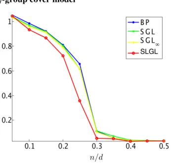
2.6.1 Sparseg-group cover model . . . 44
2.6.2 Sparse dispersive model . . . 46
2.7 Discussion . . . 47
2.8 Appendix: Review of total unimodularity . . . 49
3 Homogeneous and Non-Homogeneous Convex Relaxations 51 3.1 Introduction . . . 51
3.1.1 Related work . . . 51
3.1.2 Contributions . . . 52
3.2 Combinatorial penalties and convex relaxations . . . 52
3.2.1 Homogeneous and non-homogeneous convex envelopes . . . 53
3.2.2 Lower combinatorial envelopes . . . 55
3.3 Sparsity-inducing properties of convex relaxations . . . 58
3.3.1 Continuous stable supports . . . 58
3.3.2 Adaptive estimation . . . 60
3.4 Sparsity-inducing properties of combinatorial penalties . . . 61
3.4.1 Discrete stable supports . . . 61
3.4.2 Relation between discrete and continuous stability . . . 62
3.4.3 Examples . . . 63
3.5 Experiments . . . 64
3.6 Discussion . . . 65
3.7 Appendix: Proofs . . . 67
4 Non-Euclidean Convex Composite Optimization 79 4.1 Introduction . . . 79
4.1.1 Related work . . . 80
4.1.2 Contributions . . . 80
4.1.3 Preliminaries . . . 81
4.2 Generalized proximal gradient method: Warm-up . . . 81
4.3 Tractability of the generalized proximal operator . . . 82
4.3.1 Atomic proximal operator of polyhedral functions . . . 83
4.3.2 Proximal operator of atomic norms with linearly independent atoms . . 84
4.4 Accelerated generalized proximal gradient method . . . 87
4.5 Experiments . . . 89
4.5.1 Lasso . . . 89
4.5.2 Latent group Lasso . . . 91
4.6 Discussion . . . 93
Contents
5 Non-Convex Proximal Method for Structured Sparsity 109
5.1 Introduction . . . 109
5.1.1 Related work . . . 109
5.1.2 Contributions . . . 110
5.2 Motivating example: Graph cuts . . . 110
5.3 Discrete proximal gradient descent method . . . 112
5.4 Experiments . . . 114
5.5 Discussion . . . 115
6 MAP Estimation for Mixture Models with Combinatorial Priors 117 6.1 Introduction . . . 117
6.1.1 Related work . . . 117
6.1.2 Contributions . . . 118
6.2 Mixture model with combinatorial priors . . . 118
6.3 Majorization-minimization algorithm . . . 119
6.4 Examples . . . 121
6.4.1 Priors on the noise . . . 121
6.4.2 Priors on the continuous structure of the signal . . . 121
6.4.3 Priors on the discrete structure of the signal . . . 122
6.5 Experiments . . . 123
6.5.1 Approximately sparse Gaussian mixture model . . . 125
6.5.2 Hidden Markov tree Gaussian mixture model . . . 125
6.5.3 Sparse clustered Gaussian mixture model . . . 125
6.6 Discussion . . . 126
7 Conclusions 127 7.1 Summary . . . 127
7.2 Future directions . . . 128
Appendix A Submodular Analysis 131 A.1 Submodular functions and their Lovász extensions . . . 131
A.2 Convex closure of set functions . . . 134
Bibliography 150
1
Introduction
Learning problems are ubiquitous in machine learning, signal processing and statistics appli-cations, where given some data, we are interested in learning the underlying parameter vector. Depending on the application, the objective can be to estimate the parameter vector, or to use it for prediction or classification. In the presence of large and complicated data, solving such tasks becomes challenging, without a priori model on the data source.
Such models are particularly important in the high-dimensional setting, where the number of variables exceeds the number of observations. This setting naturally arises in modern data analysis problems, where the current trend of systematic data collection leads to a large ambient dimension. Moreover, many applications are intrinsically high-dimensional, due to observations being expensive (cost or time-wise). Without further assumptions, the learning problem in this setting is ill-posed (it admits infinitely many solutions). Fortunately, the relevant information of real-world data typically lies in a low-dimensional space. For example, in machine learning and statistics, only a small number of features are usually relevant. Similarly, in signal processing, signals can often be approximated by a small collection of basis or dictionary vectors. This idea that only few elements out of many are important is known assparsity, and has been key to the development of scalable methods that circumvent the curse of dimensionality.
While sparse modeling is powerful, it does not account for potential relationships that may exist between the variables. Indeed in many applications, the data source naturally exhibit additional structure beyond sparsity. For example, in computer vision, the pixels corresponding to the foreground of an image are expected to beclusteredtogether (see Figure 1.1), and the coefficients of the wavelet transform of an image are naturally organized on a tree (see Figure 1.2); in genomics, gene expression patterns are better explained bygroupsof genes sharing a common biological function [STM+05]. Moreover, it is sometimes advantageous to enforce additional structure. For example, in deep learning, a neural network with a compact structure, where only a fewgroupsof weights in adjacent memory space are active, is desirable to reduce computation, especially in resource constrained devices [WWW+16]. Structured sparsitymodels capture such sophisticated structures. Incorporating such models into the learning process leads to
Chapter 1. Introduction
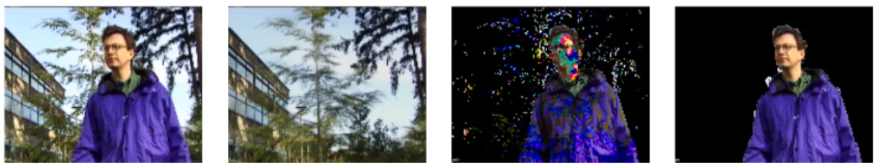
Figure 1.1: Background subtraction task: Given a sequence of frames, the goal is to segment out foreground objects in a new image. From left to right: original image; estimated background; foreground estimated with sparsity model; foreground estimated with a structured sparsity model (clustered support). This figure is taken from [MJBO10].
PSNR = 25.3538 dB PSNR = 28.0805 dB
Figure 1.2: Image inpainting task: The goal is to reconstruct the missing pixels of an image. From left to right: original image (256×256); its wavelet transform; image with 50% missing pixels; image estimated with sparsity model; image estimated with a structured sparsity model (tree support).
significant improvements in the estimation performance, as illustrated for example in Figures 1.1 and 1.2. It also leads to better noise robustness, better interpretability and allows recovery with fewer observations [EM09, BD09, CHDB09, BCDH10, HZ10, JOB10, RRN12]. To highlight the importance of the last two properties, we note that for example, obtaining more interpretable results in gene analysis, by focusing on groups of genes instead of single genes, allows biologists to identify relevant biological pathways in cancer-related data sets [STM+05]. Also, in the case of Magnetic Resonance Imaging (MRI), reducing the number of measurements allows the procedure to be shorter and thus less uncomfortable for patients [LDP07]. Moreover, sometimes observations are simply not available, like in the image inpainting task (see Figure 1.2).
The main goal of this thesis is to improve on existing structured sparsity methods and expand their success to a wider range of applications. In particular, we are interested in developing effective methods to exploit available a priori knowledge, which address the following three concerns.
• Computational efficiency: How to efficiently solve the underlying optimization problem?
• Statistical efficiency: How to reduce the number of samples needed for accurate solutions?
• Generality: How to handle a wide range of structures?
In what follows, we will first present the notation used throughout the thesis in Section 1.1, before introducing more formally the problem set-up of structured sparse learning in Section 1.2. We follow up with an overview of related work, where we identify some gaps and open problems in
1.1. Notation, terminology and prerequisites
the state-of-the-art for structured sparsity, and point out how the results presented in this thesis fill some of these gaps. In particular, we review in Section 1.3 convex approaches to structured sparsity, and in Section 1.4 two convex optimization methods for solving the resulting convex problems. In Section 1.5, we briefly review non-convex approaches to structured sparsity. We conclude the introduction with an overview of the main contributions made by this thesis. Some parts of the related work sections are based on the book chapter [KBEH+15], coauthored with Anastasios Kyrillidis, Luca Baldassarre, Quoc Tran-Dinh, and Volkan Cevher.
1.1
Notation, terminology and prerequisites
We introduce here the notation we will use throughout the thesis, and some basic terminology. We denote scalars by lowercase letters, vectors by lowercase boldface letters, matrices by boldface uppercase letters, and sets by uppercase letters.
Real-valued functions: The set of real numbers is denoted byRand the set of non-negative real numbers by R+. We write Rfor R∪ {+∞}. Given an extended real-valued function f : Rd → R, we denote its domain by dom(f) := {x ∈ Rd : f(x) < +∞}, its epigraph byepi(f) := {(x, t) ∈ Rd×R :f(x) ≤t}. We sayf isproperif its domain is non-empty, and lower semi-continuous, orclosed, if its epigraph is a closed set. We say f is positively homogeneousiff(αx) =αf(x),∀x∈Rd,∀α >0. We denote the Fenchel conjugate offby f∗, defined asf∗(x) = supy∈Rdx>y−f(y). Iff is differentiable, we denote its gradient by
∇f, and if it is non-differentiable we denote by∂fits subdifferential set. Given a setC⊆Rd, we will denote byιC(x)the indicator function of the setC, taking value0on the setCand+∞
outside it.
Convex sets and functions:A subsetC ⊆Rdisconvex, if for any two choicesx,y∈Rd, the line segment that connectsxandyalso belongs toC, i.e.,∀λ ∈ [0,1], λx+ (1−λ)y ∈ C. A function f : Rd → R is convex, if its domain is convex, and ∀x,y ∈ dom(f),∀λ ∈ [0,1], f(λx+ (1−λ)y)≤λf(x) + (1−λ)f(y). Iff is convex, then−f is calledconcave.
Set-valued functions: We consider the ground setV = {1, . . . , d}, and its power set2V =
{S|S ⊆V}composed of the2dsubsets ofV. Given a setS ⊆V, the notationScdenotes the
set complement ofSwith respect toV, and|S|its cardinality. Given a set functionF : 2V →
R, we sayF is proper if its domainD:={S :F(S)<+∞} 6=∅is non-empty, andmonotoneif
∀A⊆B⊆V, F(A)≤F(B).
Submodular set functions:A finite-valued set functionF : 2V →
Rissubmodularif and only if∀A⊆B ⊆V,∀i∈Bc,F(B∪ {i})−F(B)6F(A∪ {i})−F(A). IfFis submodular, then
−F is calledsupermodular. IfF is both submodular and supermodular, it is calledmodular.
Chapter 1. Introduction
superscriptsxkto denote thek-th vector in a sequence of vectorsx1,x2,· · ·,xk. Givenx∈Rd and a setS ⊆V,xS denotes the vector inRds.t.,[xS]i =xi,∀i∈S and[xS]i = 0,∀i6∈S.
QSSis defined similarly for a matrixQ∈Rd×d. We let1d,0dbe the vectors inRdof all ones
and all zeros, respectively, andIdthed×didentity matrix. We drop subscripts whenever the
dimensions are clear from the context. Accordingly, we let1Sbe the indicator vector of the set
S. We drop the subscript forS=V, so that1V =1denotes the vector of all ones.
We call the set of non-zero elements of a vectorxthe support, denoted bysupp(x) ={i:xi 6=
0}. We use the notation from submodular analysis, where a vectorx ∈ Rdalso denotes the modular set-function defined asx(S) =P
i∈Sxi. The symbol◦denotes the coordinate-wise
multiplication, i.e.,[x◦y]i =xiyi. Similarly the operations|x|,x≥yandsign(x)are applied
element-wise, i.e.,[|x|]i=|xi|,x≥yiffxi ≥yi,∀i∈V and[sign(x)]i=±1is the sign ofxi
withsign(0) = 0. The vector containing the positive part ofxis denoted byx+= max{x,0} (maximum taken element wise).
Inner product and norms: The inner product between two vectors x,y ∈ Rd is denoted by hx,yi = x>y = Pd
i=1xiyi. A norm of a vector xis denoted by kxk and its dual by
kxk∗ := maxkyk≤1y>x. Forp > 0, the`p-quasi-norm is given bykxkp = (Pdi=1|xi|p)1/p.
k · kp becomes a norm, ifp ≥ 1, andkxk∞ = maxi|xi|. The`0-pseudo-norm is defined as:
kxk0:=|supp(x)|. Forp∈[1,∞], we define the conjugateq∈[1,∞]via1p +1q = 1.
Prerequisites: Throughout the thesis, we make extensive use of concepts from submodular analysis. We review the relevant notions in Appendix A.
1.2
Learning with structured sparsity
We present in this section the formal set-up of the learning problems we consider in this thesis.
1.2.1 Problem set-up
In a structured sparsity learning problem, we are interested in learning a parameter vectorx\∈Rd from some noisy observationsy∈Rnthat depend onx\, wherex\is assumed to satisfy some structure, e.g, sparsity. A vectorx ∈ Rdis said to bes-sparse, if it has onlys < dnon-zero coefficients. In the commonly used linear model,yandx\are related byy=Ax\+ε, where A∈Rn×dis a known data matrix andε∈Rnis an unknown noise vector. The high-dimensional setting corresponds to the casen < d, which in the linear model example implies thatAhas a nontrivial nullspace, hence the impossibility to learnx\, even in the absence of noise, without further assumptions.
Data fidelity is typically measured by a smooth and convex loss functionf :Rd→R+, which corresponds to an empirical risk in machine learning and a data fitting term in signal processing.
1.2. Learning with structured sparsity
Examples of smooth loss functions include the square lossf(x) =ky−Axk22 in regression problems, and the logistic lossf(x) =Pn
i=1log(1 + exp(−yixTai))in classification problems.
Structured sparsity models are inherently combinatorial, and can thus be naturally encoded by set functionsF : 2V →
R∪ {+∞}defined on the supportsupp(x) ={i:xi6= 0}. Incorporating
such prior information in learning problems leads then to the following problem: min
x∈Rd
f(x) +λF(supp(x)), (1.1)
whereλ≥0is a regularization parameter that controls the trade-off between data-fitting and regularization. F(supp(x))then favors certainsupports, ornon-zero patterns, over others. For example, to favor sparse supports, the`0-pseudo-normF(supp(x)) =|supp(x)|can be used. To enforce hard constraints,F can be chosen to be an indicator function over a set of allowed supports; e.g.,F(supp(x)) =ι|supp(x)|≤s(x). Problem (1.1) is computationally intractable1in
general (see e.g., [Nat95]). Two main approaches, each with its own merits and shortcomings, have been adopted in the literature to confront this computational challenge. One is vianon-convex approachesthat provide approximate solutions directly to (1.1). The other is based on continuous convex relaxationswhereF(supp(x))is replaced by a convex surrogateg:Rd→R∪ {+∞}, yielding the followingcomposite convex minimizationproblem:
min
x∈Rdf(x) +λg(x), (1.2)
The main benefit of non-convex approaches is that, by maintaining the combinatorial term in problem (1.1), they preserve the true structure model. This is particularly important in the case of structures that have no meaningful convex relaxations (such cases are identified in Chapter 3). Existing non-convex methods are based on iterative greedy algorithms, which are guaranteed to return approximate solutions to (1.1), but are only known to be tractable in special cases of structures. See Section 1.5 for further details.
Convex methods on the other hand can utilize a rich set of algorithmic tools guaranteed to return solutions of arbitrary accuracy to the relaxed convex problem (1.2), and analysis tools for characterizing the statistical efficiency of the resulting estimator. They also tend to be more robust tomodel misspecifications, which is likely to occur in practice.
The challenge in this approach resides in finding a convex surrogate, which can be efficiently optimized, while still preserving the structure encoded by F, which is crucial to guarantee statistical efficiency. We present some of the convex surrogates proposed in the literature to achieve this in Section 1.3, and review some methods to optimize the resulting convex problems in Section 1.4.
We will adopt the convex approach to structured sparsity throughout most of the thesis, except 1Throughout the thesis, we will use “intractable” to mean NP-Hard.
Chapter 1. Introduction
for the last two chapters, where we turn to non-convex approaches to handle structures with no meaningful convex relaxations.
1.2.2 Performance criteria
As we mentioned earlier, throughout the thesis, when considering an approach for learning with structured sparsity, we will be concerned with three factors: Computational efficiency, statistical efficiency, and generality. We now clarify what is meant by the first two notions.
Given a choice ofF org, and a solutionxˆ returned by a proposed algorithm solving the corre-sponding optimization problem. Statistical efficiency is concerned with the number of samples required forxˆ to estimatex\and its support, up to some target accuracy, while computational
efficiency is concerned with the time needed to achieve this.
Let x? be a minimizer2 of problem (1.1) for non-convex methods, and of problem (1.2) for convex ones, andL?the corresponding optimal objective value, e.g.,L?=f(x?) +λg(x?)in the convex approach case. We will split the discussion into the following two parts, as is often done in classical convex approaches3.
Optimization performance: Given a proposed iterative4 algorithm, letxk be the solution obtained at an iterationkof the algorithm. We are interested in assessing the scalability of the algorithm with respect to the following, often conflicting, criteria:
• Computational cost per iteration: The performance of an iterative algorithm highly depends on the cost of computing xk at each iteration, in terms of dependence on the
dimensionsdandnof the problem.
• Number of iterations: The performance of an iterative algorithm also depends on the number of iterations required to obtain a target numerical accuracy > 0, either with respect to the objective error, i.e., L(xk)− L? ≤or the distance to the optimal point
(if unique), i.e.,kxk−x?k ≤. The number of iterations typically depends both on the accuracyand the dimensionsdandnof the problem.
Note that, in large scale optimization problems, such as the ones considered in this thesis, the dependence in the above two criteria on the ambient dimensiondis particularly important.
Statistical performance: We are interested in studying the performance ofx?as an estimator of x\ in terms of the following criteria, where the probability is with respect to all random
2
Without further assumptions,x?is not necessarily unique.
3
Modern stochastic methods in machine learning tackle the computation and analysis ofxˆsimultaneously.
1.2. Learning with structured sparsity
elements in the problem (e.g., noise and design matrix). For formal definitions, see, e.g., [Liu10].
• Estimation consistency:We say thatx?is estimation consistent, if theestimation error, i.e.,kx?−x\kconverges in probability to zero.
• Model selection consistency: This criterion is also called sparsistency. We say thatx? is sparsistent, if thesupport recovery error, i.e.,k1supp(x?)−1supp(x\)k0 converges in probability to zero.
In the asymptotic regime,dis finite and fixed, and convergence in the above two criteria is with respect ton→ ∞. This regime forbids the high-dimensional setting, and is thus less interesting in the context of structured sparsity. Nevertheless, studying it typically requires simpler analysis, and is helpful to develop insights which contribute to the understanding of the high-dimensional setting. In thenon-asymptoticregime, we are interested in the rate of convergence of the errors in the above two criteria, as a function of the ambient dimensiond, the number of samplesn, and the sparsitys=|supp(x\)|(or more generally the “complexity” ofx\under the assumed structured sparsity model). In particular, the number of samples required to recover (up to some accuracy) x\, as a function ofdandsis calledsample complexity. Other performance criteria, such as prediction error, are also of interest, but we will focus on these two criteria in our discussion.
1.2.3 Penalized and constrained formulations
Note that by allowing F and g to take infinite values, problems (1.1) and (1.2) include two regularization variants. Given our convex loss functionf and a regularizerΩ : Rd → R, the penalized variant, also known as the Lagrangian form, is given by:
min
x∈Rdf(x) +λΩ(x), (1.3)
while the constrained variant is given by: min
x∈Rd{f(x) : Ω(x)≤τ}. (1.4)
IfΩis convex then, under some mild conditions, the two variants are equivalent, in the sense that x?is a solution of problem (1.3) for someλ >0, if and only if, it is a solution of problem (1.4) for someτ >0[BL10, Sect. 4.3]. However, the exact relation betweenλandτ is not known. In practice, the choice between one or the other variant, depends on factors such as computational complexity, stability, and robustness. For example, depending onΩ, one variant can be easier to solve than the other. Moreover, the solution of problem (1.3) is less sensitive to small changes in λ, than the solution of problem (1.4) to small changes inτ, which makes tuningλeasier than tuningτ, in practice. Also, whenf is the least squares loss, the penalized formulation can be more robust to model misspecifications [LST13]. In these cases, the penalized formulation is
Chapter 1. Introduction
thus preferable. On the other hand, if one is interested in enforcing a fixed boundτ onΩ(x)≤τ, the constrained formulation is then preferable. This is particularly relevant in the non-convex setting, where we might be interested for example in obtaining solutions that are exactlys-sparse.
1.3
Convex approaches
In this section, we present several approaches adopted in the literature to design convex surrogates of structured sparsity models. In each case, we will pay attention to the structures that can be expressed by the presented convex penalty and its statistical properties, if known. We defer the discussion of how to optimize the resulting convex problems to Section 1.4.
1.3.1 Popular structured sparsity-inducing norms
A classical approach for choosing a convex surrogate consists of designing a norm that leads to the desired set of non-zero patterns in a “reverse-engineering” manner. This approach led to the design of several interesting structured sparsity-inducing norms. We outline below some of them
Lasso (`1-norm)
We start with the most popular example of sparsity-inducing norms, the`1-norm, which is used as a convex surrogate of the`0-pseudo-norm. In this case, whenf is the least-squares loss, problem (1.2) reduces to the following formulation, known as basis pursuit denoising (BPDN)5[CDS98].
min x∈Rd 1 2ky−Axk 2 2+λkxk1. (1.5)
Another closely related formulation is known as the least absolute shrinkage and selection operator (Lasso) [Tib96]:
min x∈Rd{ 1 2ky−Axk 2 2 :kxk1 ≤τ}. (1.6)
In Sections 1.3.3 and 1.3.4, we present a formal justification as to why the`1-norm is the “best” convex surrogate for the`0-pseudo-norm. We present here some intuitive reasons for why the`1 -norm induces sparsity. From an analytical perspective, we can see this by considering the simple denoising example, whereA=I in the BPDN formulation (1.5). The solution in this case is given by the soft-thresholding operator, introduced by [DJ95],x?(λ) = sign(y)◦max{|y|−λ,0}.
For large enough λ, x?(λ) is sparse, since all coefficients |yi| ≤ λ are set to zero. This
behavior mimics the solution obtained by regularizing instead with the`0-pseudo-norm,x?(λ) = y◦1{i:|yi|≥√
2λ}, where all coefficients|yi| ≤
√
2λare set to zero. The difference between the 5BPDN is also sometimes used to refer to the following formulation:min
x∈Rd{kxk1:ky−Axk
2 2≤τ}.
1.3. Convex approaches
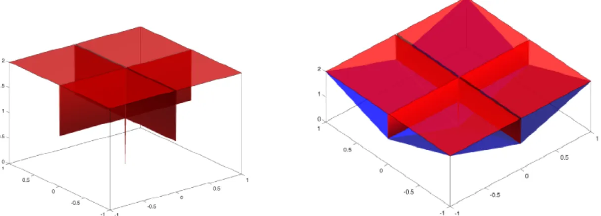
Figure 1.3: Unit balls of`0-“norm”, restricted to the unit`∞-ball (left), and`1-norm (right).
two solutions is the additional shrinkage effect imposed in the`1-solution.
From a geometric perspective, it is easy to see that the unit `1-ball is the convex hull of the standard basis vectors, which are one-sparse, or equivalently of the unit`0-ball, when restricted inside the unit`∞-ball, i.e., the set{x:kxk0 ≤1,kxk∞ ≤1}(see Figure 1.3). In fact, from this perspective,`1-norm is a special case of a class of norms defined as convex hulls of vectors whose support satisfy the desired structure, which we discuss in Section 1.3.2.
The convex approach proved to be successful in this case. Indeed, replacing the`0 -pseudo-norm with the`1-norm, allows efficient robust recovery of anys-sparse vectorx\∈Rd, in the linear model case, using onlyn=O(slog(d/s))samples, under some assumptions onA(e.g., restricted isometry property) [CT05, Don06].This sample complexity can be significantly smaller than the classical Shannon-Nyquist sampling bound, which dictates uniformly sampling a signal at a rate at least twice its highest frequency in the Fourier domain [Sha49].
In the past decade, substantial work was done towards extending this success to more involved structures, with various convex penalties proposed in the literature (see [OB16] and [KBEH+15] for an overview).
Group Lasso
A simple extension of the Lasso is the group Lasso [YL06], also called`1/`p-norm, defined as:
Ω∩p(x) = X
G∈G
dGkxGkp, (1.7)
whereGis a collection of non-overlapping groups that partitionV,(dG)G∈Gare positive weights,
and wherep≥1, withp∈ {2,∞}being popular choices in practice. Ω∩
p acts as an`1-norm (when weights are equal) over the termskxGkp, and hence it promotes
sparsity on the group level. This structure, dubbed as block-sparsity, was shown to improve the estimation performance over standard Lasso, when x\ is block-sparse, both in terms of sampling complexity and noise robustness [SPH09, EB09, HZ10]. Block-sparsity arises in applications such as DNA microarrays [PVMH08], equalization of communication channels [CR02], multi-task learning [OTJ10], and multiple kernel learning [Bac08].
Chapter 1. Introduction
Figure 1.4: Unit ball of`1/`∞-norm (left) and`∞-LGL norm (right), forG={{1,2},{2,3}}.
Figure 1.5: The sets in blue or green are the groups to include inG, along with their complements, to select interval (left) or rectangular (right) patterns, as proposed in [JAB11]. The sets in red are examples of the corresponding induced non-zero patterns. This figure is taken from [OB16].
Group Lasso was further generalized to the case of overlapping groups in [ZRY09, JOV09, JAB11, MJOB11]. Figure 1.4 (left) displays the unit `1/`∞-norm ball, for an example of overlapping groups. This norm was shown, in [JAB11], to induce supports corresponding to the intersectionof a sub-collection of the complements of groups inG. Conversely, given a intersection-closed6set of non-zero patterns, it is possible to engineer the groups inGin order to favor these patterns viaΩ∩p.
For example, [JAB11] showed that using the groups displayed in Figure 1.5 (left) inducesinterval patterns; a structure desirable in applications such as time series, or cancer diagnosis [RBV08]. Similarly, using the groups displayed in Figure 1.5 (right) induces rectangular patterns; a struc-ture desirable in applications such as background subtraction [CHDB09, MJBO10], dictionary learning [MJOB11] and face recognition [JOB10]. Ω∩
p can also be used to induce hierarchical
structures which we discuss below. The statistical properties ofΩ∩
p were studied in [JAB11], with conditions for consistent estimation
of the non-zero patterns presented, both in low and high-dimensional settings. In Section 1.3.3, we see why the overlapping `1/`∞-norm is the “best” convex surrogate, in some sense, for group-intersection structures.
Latent group Lasso
As mentioned above, overlapping`1/`p-norm can induce supports belonging to an
intersection-closed set of supports, while in several applications, non-zero patterns corresponding to the 6A setSis intersection-closed if∀S
1.3. Convex approaches
Figure 1.6: Unit ball ofΩ∩
∞(left), and corresponding groupsGH ={{1,2,3},{2},{3}}(right).
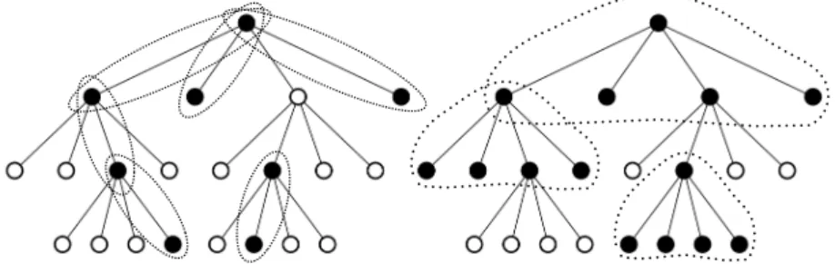
Figure 1.7: Examples of parent-child and family models. Active groups are indicated by dotted ellipses. The support (black nodes) is given by the union of the active groups. (Left) Parent-child model. (Right) Family model.
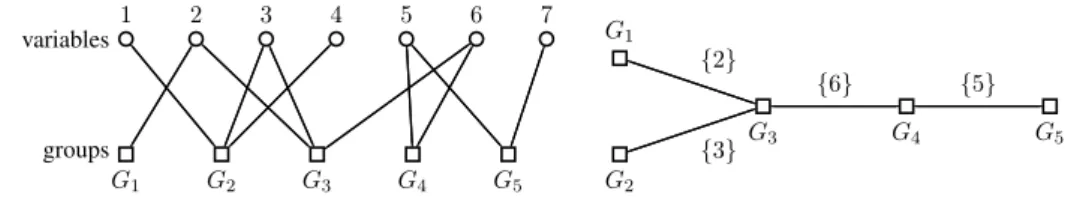
unionof a sub-collection of groups inGare more desirable. This is particularly important, in applications such as cancer prognosis from high-dimensional gene expression data, where the groups are naturally predefined, e.g., genes involving the same biological function should be grouped together, as opposed to being manually chosen. This motivated another generalization of group Lasso to overlapping groups, given by the latent group Lasso (LGL), introduced by [JOV09] (see also [OJV11]). Given a collection of groupsG, and associated positive weights (dG)G∈G, the LGL norm is defined as;
Ω∪p(x) = min v∈Rd×|G|{ X G∈G dGkvGkp : X G∈G vG=|x|,supp(vG)⊆G}. (1.8)
Note thatΩ∪p andΩ∩p are equal in the case ofnon-overlappinggroups, but in general they are different, as it is apparent for example from Figure 1.4. Ω∪p can also be used to induce hierarchical structures as we discuss next.
A detailed analysis ofΩ∪p and its statistical properties, in terms ofgroup-supportrecovery, in the low-dimensional setting, is presented in [OJV11]. In Sections 1.3.4 and 2.5.1, we see why the latent group Lasso is the “best” convex surrogate, in some sense, for group-cover structures.
Hierarchical sparsity
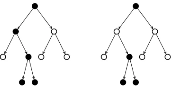
In a hierarchical sparsity model, the variables or groups of variables are organized over a directed tree, (or a forest)T, and they satisfy hierarchical relations, e.g., an element can be selected only
Chapter 1. Introduction
if all its ancestors inT are also selected; this is known as the rooted connected tree structure. The more general case where variables are organized over a directed acyclic graph was also studied, see, e.g., [YB+17] and [OB16].
Hierarchical structures are found in many applications, such as image processing, to exploit the multi-scale structure of wavelet coefficients, see Figure 1.2 and [DWB08, ZRY09, BCDH10, JMOB11]; bioinformatics, to leverage the hierarchical structure of gene networks for multitask regression [KX10]; deep learning, where hierarchies of latent variables are used in convolutional neural networks [Ben09].
Such structure was shown to result in better performance than standard Lasso, both in terms of noise robustness and sample complexity. In particular, [BCDH10] showed that we can recover anys-sparse vectorx\∈
Rdthat satisfies a rooted connected tree structure, using onlyn=O(s) samples, in the linear model case, and under similar assumptions onAas in Lasso.
Both overlapping group Lasso and latent group Lasso were used in the literature to induce hierar-chical structures. In particular, if we define groups inGH as each node and all itsdescendants
inT, then the correspondingΩ∩
p results in the hierarchical group lasso [ZRY09]. Figure 1.6
displays an example of the descendants groups and the corresponding unit ball ofΩ∩∞. In Section 2.5.2, we see why the`∞-hierarchical group Lasso is the “best” convex surrogate, in some sense, for the rooted connected tree structure.
On the other hand, the latent group Lasso norm was used with groups defined inGAas each node and all itsancestorsinT, to induce hierarchical structures. A systematic comparison ofΩ∩
2 with
GH, andΩ∪2 withGA, and their statistical properties, is presented in [YB+17]. In particular, it
is shown that though the two penalties are not identical with these groups, they do lead to the same class of non-zero patterns, with the difference that group Lasso shrink more aggressively parameters deep in the hierarchy.
Other group structures were also used with the latent group Lasso norm. For example, a parent-child model, where groups consist of all parent-parent-child pairs in T (see Figure 1.7, left), and a family model, where groups consist of each node and all its children (see Figure 1.7, right), were proposed in order to favor tree-structures, but also allowing for a certain degree of flexibility in deviations from the rooted connected tree structure [BBC+16, RNWK11].
Exclusive Lasso
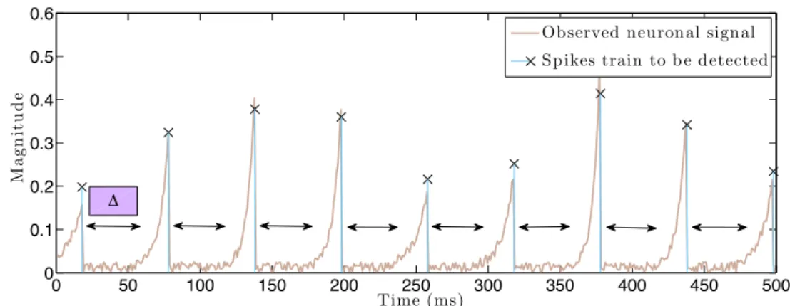
In certain applications, it is desirable to induce non-zero patterns, where sparse coefficients within a group compete against each other, i.e., a non-zero entry discourages other entries, within the same group, to be non-zero. For example, this structure naturally arises in neurobiology. Inspired by the statistical analysis in [GK02], the authors in [HDC09] consider a simple one-dimensional model, where a neuronal signal behaves as a train of spike signals with some refractory period ∆>0: there is a minimum non-zero time period∆where a neuron remains inactive between
1.3. Convex approaches 0 50 100 150 200 250 300 350 400 450 500 0 0.1 0.2 0.3 0.4 0.5 0.6 Time (ms) Ma g n it u d e
Observed neuronal signal Spikes train to b e detected
Figure 1.8: Neuronal spike train example
two consecutive electrical excitations. Figure 1.8 illustrates how a collection of noisy neuronal spike signals with∆>0might appear in practice.
The exclusive Lasso, also called`p/`1-norm, proposed by [ZJH10]7, promotes suchdispersive structure. Given a collection of groupsG, and associated positive weights(dG)G∈G, exclusive
Lasso is defined as:
Ωexclusive p (x) = ( X G∈G kxGkp1) 1/p. (1.9) Ωexclusive
p acts as an`1-norm on each group, and thus promotes sparsity within each group. In Sections 1.3.4 and 2.5.3, we see why the exclusive Lasso is the “best” convex surrogate, in some sense, for dispersive structures.
1.3.2 Atomic norms
A more principled general approach for choosing a convex surrogate of a structured sparsity model was proposed in [CRPW12]. This approach considers models wherex\is “simple” in the sense that it can be written as the sum of a fewatomsfrom an atomic setA, with possibly infinite atoms, i.e.,x\ =Ps
i=1ciai. The proposed convex penalty is then given by the gauge of
the convex hull of the atomic set:
kxkA = inf{t≥0 :x∈tconv(A)}, (1.10) which, assuming without loss of generality that the centroid ofAis zero, can be rewritten as:
kxkA = inf{ X a∈A ca :x= X a∈A caa, ca≥0,∀a∈ A}, (1.11)
kxkAis a norm, called theatomic norm, wheneverAis centrally symmetric around the origin, i.e., when a ∈ A if and only if −a ∈ A. This convex penalty is in general intractable to
Chapter 1. Introduction
evaluate and to optimize (e.g., when conv(A)is the cut polytope), but for certain cases ofA it can be evaluated exactly, or approximated via semidefinite programming, and the resulting convex optimization problems are tractable (see [CRPW12] for details). Moreover, for certain choices ofA, the atomic norm recovers popular structured sparsity-inducing norms, such as:
(i) `1-norm:IfAis the set of standard basis vectors, i.e.,A={a∈Rd:kak0 = 1,kakp ≤
1}(for anyp≥1), thenkxkA =kxk1.
(ii) Latent group Lasso norm:For a collection of groupsG, and positive weights(dG)G∈G,
ifA={a∈ Rd : supp(a) ⊆G,kakp =d−1G , for someG∈G}, thenkxkA = Ω∪p(x)
defined in Eq. (1.8), as shown in [OB12].
Furthermore, Section 1.3.4 introduces another class of structure-inducing norms, which can be viewed as atomic norms too. For other interesting examples, we refer the reader to [CRPW12]. Conditions for exact and robust recovery ofx\using general atomic norms, along with bounds
on the corresponding sample complexity are presented in [CRPW12].
The main drawback to this approach is that the proposed convex penalties are gauge functions and thus are necessarily positively homogeneous; we discuss why this is problematic, in terms of capturing general structures, in Chapters 2 and 3.
1.3.3 Convex relaxations of submodular penalties
Another systematic approach, proposed in [Bac10a], considers choosing the convex surrogate to be the tightest convex relaxationof the desired structured sparsity model. Namely, given a positive-valued set function F : 2V →
R+, such thatF(∅) = 0, andF(A) > 0,∀A ⊆ V, encoding the structure on the support of x ∈ Rd, this approach proposes to use theconvex envelope of F(supp(x)), i.e., its largest (thus tightest) convex lower bound8, over the unit `∞-ball, as a natural convex surrogate for it.
In particular, this approach is applied in [Bac10a] for structures that can be expressed by a monotone submodular function (see definitions in Section 1.1). The convex envelope of a function is given by its biconjugate, i.e., the Fenchel conjugate of the Fenchel conjugate. Let F∞(x) =F(supp(x)) +ιkxk∞≤1(x), then the convex envelope ofF∞is given byΘ∞:=F
∗∗ ∞. Note that restricting the values of xto a bounded domain (e.g., unit `∞-ball) is a necessary technical requirement for deriving non-trivial relaxations of such functions. Unfortunately, the convex envelopeΘ∞is in generalintractableto evaluate and to optimize9. However, for the class of monotone submodular functions, [Bac10a] shows thatΘ∞is given by theLovász extension
8Throughout the thesis, we will thus use convex envelope and tightest convex relaxation interchangeably. 9
We can see this for example from the connection between the convex envelope ofF∞and the convex closure of
1.3. Convex approaches
Figure 1.9: `0-pseudo-norm (red) and its convex envelope over the unit`∞-ball; the`1-norm (blue), inR2.
[Lov83] ofF,Θ∞(x) =fL(|x|), wherefLis defined as follows:
fL(x) = d−1
X
k=1
xjk[F({j1, . . . , jk})−F({j1, . . . , jk−1})], (1.12) wherexis sorted in decreasing orderxj1 ≥ · · · ≥xjd. WhenF is submodular,fLis known to be convex. For further details about the Lovász extension see Appendix A.1.
We can see from the definition of the Lovász extension in (1.12), thatΘ∞in this case is a norm, and is efficiently computable. Tractable algorithms to solve the resulting convex optimization problems, regularized withΘ∞, are also proposed in [Bac10a] (see also Section 1.4.1). Moreover, for certain choices of the submodular function F, Θ∞ recovers popular structured sparsity-inducing norms, such as:
(i) `1-norm:IfF is the cardinality function,F(S) =|S|, thenΘ∞(x) =kxk1. Figure 1.9 displays the`0-pseudo-norm, restricted within the`∞-ball, and its convex envelope the `1-norm. It is easy to see from this figure, why considering the convex envelope over an unbounded domain would simply yield the zero function.
(ii) `1/`∞-norm: For a collection of groupsG, and positive weights(dG)G∈G, ifF is the
overlap count function,F(S) =P
G∈G,G∩S6=∅dG, thenΘ∞= Ω∩∞, defined in Eq. (1.7). For other interesting examples, we refer the reader to [Bac10a]. In Chapter 2, we show that this approach is also tractable for another class of interesting set functions.
Note that the approach outlined here is similar to the one in Section 1.3.2, in the sense that both approaches attempt to compute the “best” convex surrogate of a given structured sparsity model. Indeed, the notion of convex envelope extends the notion of convex hull of sets to functions. In
Chapter 1. Introduction
particular, the epigraph of the convex envelopeΘ∞corresponds to the closure of the convex hull of the epigraph ofF∞. Moreover, the atomic normkxkAof a compact atomic setAis the convex envelope of the functionx→ inf{t≥0 :x∈tA}. However, a key difference is that, unlike atomic norms, convex penalties obtained as convex envelopes ofF(supp(x))are not necessarily norms, whenF is not monotone submodular, as we show in Chapter 2. In that chapter, we identify another class of set functions, for which the convex envelopeΘ∞is efficiently computable. The statistical properties ofΘ∞, with conditions for support recovery and estimation, in the high dimensional setting, are presented in [Bac10a]. In particular, it is shown that the non-zero patterns allowed with these norms correspond to thestablesets ofF, i.e., setsA⊆V that satisfy
∀B ⊃A, F(B)> F(A).
1.3.4 Homogeneous convex relaxations of`p-regularized penalties
A similar principled approach to the one discussed above, proposed in [OB12], considers`p
-regularized general combinatorial functions of the formFp(x) = 1qF(supp(x)) +1pkxkp, for
p ≥ 1, where as before the set function F controls the structure of the model in terms of allowed/favored non-zero patterns, and the additional`p-norm serves to control the magnitude of
the coefficients. Forp=∞,Fpreduces toF∞(x) =F(supp(x)) +ιkxk∞≤1(x). The choice
p 6=∞might be preferable to avoid the clustering artifacts of the values of the learned vector induced by the`∞-norm.
This approach proposes to use the largestpositively homogeneousconvex lower bound ofFpas a
convex surrogate for it. This is achieved by computing first the positively homogeneous envelope of Fp, i.e., its largest positively homogeneous lower bound, given by F(supp(x))1/qkxkp,
then computing the corresponding convex envelope. We call the resulting convex penalty the homogeneous convex envelopeofFp, and denote it byΩp.
[OB12] showed that the homogeneous convex envelope ofFp, for any set functionF, is given by
ageneralized latent group Lasso norm:
Ωp(x) = min v { X S⊆V F(S)1/qkvSkp : X S⊆V vS =|x|,supp(vS)⊆S}. (1.13) Note that the norm in Eq. (1.13) indeed corresponds to a latent group Lasso norm as defined in Eq. (1.8), withGcontaining all the power-set ofV. Moreover,Ωpcan be viewed as an atomic norm,
associated with the atomic setA ={a ∈ Rd : supp(a) ⊆S,kakp = 1, for someS ∈ DF},
whereDF is thecoreset ofF, corresponding to the set of faces of a polytope associated withΩp.
See [OB16, Section 2.3] for the precise definition.
Unfortunately, the homogeneous convex envelopeΩp is also in generalintractableto evaluate
and to optimize. However, ifFis a monotone submodular function, a tractabledecomposition algorithmto computeΩp for anyp≥1, was provided in [OB16, Section 6.3]. This algorithm
1.4. Convex optimization for structured sparsity
requires solving a sequence of at mostdsubmodular minimization problems, which can be done in polynomial time for general submodular functionsF (see Section A.1). Tractable algorithms to solve the resulting convex optimization problems, regularized withΩp, are also proposed in
[OB16] (see also Section 1.4.1). Moreover, for certain choices ofF (including non-submodular ones),Ωprecovers popular structured sparsity-inducing norms, such as:
(i) `1-norm:IfF is the cardinality function,F(S) =|S|, thenΩp(x) =kxk1foranyp≥1. (ii) Submodular norms: IfF is monotone submodular, then the homogeneous convex enve-lope coincides with the convex enveenve-lope, whenp=∞, i.e.,Ω∞= Θ∞=fL(| · |), and it
is then easily computable (the decomposition algorithm is not needed in this case). For generalpthough, the two envelopes are not necessarily equal (see next example).
(iii) `1/`p-norm: For a collection of groupsG, and positive weights (dG)G∈G, ifF is the
submodular overlap count function,F(S) =P
G∈G,G∩S6=∅dG, thenΩp= Ω∩p, defined in
Eq. (1.7), only ifGis a partition ofV. Otherwise, for overlapping groups, this identity does not hold forp <∞. In this case, the norm, called overlap count Lasso, does not have a simple closed form in general (but it can be computed using the decomposition algorithm). For more details on the difference between overlap count Lasso and`1/`p-norms, see
[OB16, Section 4.1].
(iv) Latent group Lasso norm: IfF is the (non-submodular) minimal weighted set cover function,F(S) = minω∈{0,1}|G|{PG∈GdGωG : PG∈GωG1G ≥ 1S}, thenΩp = Ω∪p,
defined in Eq. (1.8). Note that this norm is not tractable in general (e.g., whenG= 2V
as in Eq. (1.13), but for example if the number of groups inGis polynomial, it can be computed by linear programming.
(v) `p/`1-norm:IfF is the (non-submodular) functionF(S) = maxG∈G|S∩G|, andGis a
partition ofV, thenΩp = Ωexclusivep , defined in Eq. (1.9).
For other interesting examples, we refer the reader to [OB16]. An extension of the statistical results presented in [Bac10a] forΘ∞, in the case of monotone submodular functions, toΩp for
the same class of functions, with anyp≥1, is provided in [OB16].
This approach has a similar drawback to the approach of atomic norms, namely that the proposed convex penalties are necessarily positively homogeneous; we discuss why this is problematic, in terms of capturing general structures, in Chapter 3. In that chapter, we study the non-homogeneous counterpart ofΩp, i.e., the convex envelope ofFp, for general set functions, and anyp≥1.
1.4
Convex optimization for structured sparsity
In the previous section, we reviewed existing approaches to convert the combinatorial termF in problem (1.1) to a convex termg. The resulting convex penalties are naturallynon-smooth. In
Chapter 1. Introduction
this section, we review two first-order methods10tailored to optimize the corresponding convex problem (1.2), wherefis a smooth differentiable function, andgis a non-smooth convex function. In particular, f is assumed to have a Lipschitz continuous gradient with respect tok · k, i.e.,
k∇f(x)− ∇f(y)k∗ ≤Lkx−yk,∀x,y ∈Rd, for someL > 0, and wherek · k∗is the dual norm ofk · k. In some cases,fcan be further assumed to bestrongly-convexwith respect tok · k, i.e.,f(x)≥f(y) +hx−y,∇f(y)i+µ
2kx−yk
2,∀x,y∈
Rd, for someµ >0.
In large-scale problems, first-order methods are often preferred to second-order methods, despite requiring a larger number of iterations to achieve a given accuracy, due to their lower-complexity per iteration. In the context of structured-sparsity, existing first-order optimization algorithms often fall under the categories ofproximal gradient methods(also known asforward–backward splittingmethods) andFrank-Wolfe(FW) methods (also known asconditional gradient methods). In what follows, we present these two methods, and highlight their respective advantages and drawbacks. For each method, we will pay attention to its computational complexity per iteration, its convergence rate guarantees, the sparsity of its solutions, and its ability to handlegeneral norms. Our interest in the last two properties is motivated by the following: First, optimization algorithms which maintain sparse iterates are desirable in structured sparsity problems, where we indeed seek sparse solutions, but also in general large-scale problems, due to the computational benefit this property entail. Second, algorithms which allow arbitrary choices of the normk · k, instead of the classical`2-norm, enable us to adapt the norm to the geometry of the given problem. This property can lead to significant improvement in the convergence rate in terms of dimension dependence, as observed for example in [KLOS14, Nes05, BWB14, dGJ13].
1.4.1 Proximal gradient methods
Proximal methods date back to [Mar70]. They have received a lot of attention both from the machine learning and signal processing communities, see, e.g., [WNF09, MRS+10, Bac10b, CP11], due to their relatively fast convergence rate and their suitability for large-scale non-smooth convex problems of the form (1.2).
Algorithm: The main idea of proximal gradient methods is to minimize at each iterationk, a quadratic approximation off, tight at the current iteratexk, while leavinggintact. Assuming the gradient off isL2-Lipschitz continuous, with respect to the`2-norm, implies the following quadratic majorizer off, at any pointy∈Rd, and∀γ ∈(0,1/L2]:
f(x)≤f(y) +hx−y,∇f(y)i+ 1
2γkx−yk 2
2. (1.14)
1.4. Convex optimization for structured sparsity
The following problem is then solved at each iterationk:
min x∈Rd 1 2γkkx−(x k −γk∇f(xk))k22+λg(x) (1.15) In the basic proximal gradient method, the next iterate is set to the unique (by strong convexity) solution of (1.15). In the special case wheregis an indicator functiong= ιC, this algorithm
is calledprojected gradient method, since problem (1.15) reduces to a projection onC. Also if g= 0, we recover the standard gradient descent algorithm. Accelerated variants of the proximal gradient method, such as [Tse08, BT09a, Nes13], include an additional extrapolation step. For example, one simple version is to set the next iterate to the solution of problem (1.15) withxk replaced withxk+αk(xk−xk−1), for some carefully chosenαk∈(0,1].
When the Lipschitz constantL2 is not known, the step sizeγk can be found by line search. For example, one simple line search strategy, proposed by [BT09b, Section 1.4.3], consists of iteratively increasingγkuntil the bound in (1.14) holds. Such adaptive choice of the step size
can be helpful even in cases whereL2 is known, because it allows the algorithm to adapt to the local properties of the objective.
The solution of (1.15) corresponds to an instance of theproximal operator[Mor62] ofg:
proxλg(u) := arg min
x∈Rd 1
2kx−uk
2
2+λg(x) (1.16)
Whengis an indicator functiong=ιC, Eq. (1.16) becomes a projection onC, and is denoted
byprojC(u). Note that this operator is well-defined, since the solution in (1.16) is unique. The iterates of the basic proximal gradient method can then be written as
xk+1= proxλg(xk−γk∇f(xk)), and that of its simple accelerated variant as
yk+1 =xk+αk(xk−xk−1),
xk+1 = proxλg(yk+1−γk∇f(yk+1)).
Complexity per iteration: The cost per iteration of proximal gradient methods is dominated by the cost of computing the proximal operator. This operator has several nice properties which are helpful for computing it, and for establishing convergence of proximal methods, see e.g., [CW05]. We review here one particular property, known as theMoreau decomposition, which relates the proximal operator ofgto the one associated with its Fenchel conjugateg∗:
Chapter 1. Introduction
This relation allows us to efficiently compute both proximal operators, whenever one of them is efficiently computable. In the special case whereg=k · kis a norm, theng∗ =ιk·k∗≤1, and Eq.
(1.17) reduces to
u= proxk·k(u) + projk·k∗≤1(u). (1.18)
For some choices of structured sparsity-inducing norms, the proximal operator can be computed efficiently. We present now some of these examples:
(i) `1-norm: proxλk·k1 has a closed form solution, given by proxλk·k1(u) = sign(u)◦ max{|u|−λ,0}. This is the soft-thresholding operator we presented in Section (1.3.1). The proximal gradient method in this case is often called ISTA (iterative shrinkage-thresholding algorithm), and its accelerated variant FISTA (fast ISTA) [BT09a].
(ii) Submodular norms:Ifgis the norm obtained from the convex envelopeΘ∞or the homo-geneous convex envelopeΩpof a monotone submodular function (see Sections 1.3.3 and
1.3.4)11, then its proximal operator can be computed by adecomposition algorithm[OB16, Section 6.3]. As in the decomposition algorithm used to compute the norm itself, this algorithm requires solving a sequence of at mostdsubmodular minimization problems. (iii) Block`1/`p-norm:IfGis a partition ofV, the proximal operator ofΩ∩p, defined in Eq.
(1.7), can be computed separately on each group;[proxλΩ∩
p(u)]G= proxλdGk·kp(uG),∀G∈
G. Forp= 2, we obtain the group soft-thresholding operator[proxλΩ∩
2(u)]G = sign(uG)◦ max{kuGk2−λdG,0}. Forp=∞, the relation in Eq. (1.18) can be exploited to compute
[proxλΩ∩
∞(u)]Gas the residual of the Euclidean projection on the`1-ball, which can be
done in linear time [DSSSC08].
(iv) Hierarchical`1/`p-norm: If the groups inGare tree-structured, in the sense that every
pair of groups are either disjoint or one is contained in the other, [JMOB11] provided efficient algorithms to compute proxλΩ∩
p(u) for p = 2,∞. The algorithm consists of sequentially projectinguGon the dual ball, given a particular ordering of the groups. The
resulting complexity isO(d)forp= 2, andO(dh)wherehis the height of the tree. For example, this applies to the rooted connected tree model presented in Section 1.3.1, where the descendant groupsGH are indeed tree-structured.
(v) Overlapping `1/`p-norm: If the groups in Gare overlapping and not-tree structured,
proxλΩ∩
p(u)becomes more difficult. It can still be solved efficiently in the special case of p=∞, whereproxλΩ∩
∞(u)is the dual to a quadratic min-cost flow problem, as shown in
[MJBO10]. Alternatively, the decomposition algorithm can be used, since`1/`∞-norm is a submodular norm (see Section 1.3.4). However, in the general case wherep∈(1,∞), no efficient algorithm to computeproxλΩ∩
p is known.
(vi) Latent group Lasso norm:IfGis a partition ofV, recall thatΩ∪p, defined in Eq. 1.8, is equal to the`1/`p-norm, hence its proximal operator can be easily computed in this case.
11Recall that the two envelopes are equal forp=∞;Θ
1.4. Convex optimization for structured sparsity
However, in the overlapping-groups case, computingproxλΩ∪
p is challenging. A simple workaround is to duplicate the variables that belong to overlaps between the groups, which reduces this case back to the partition case. However, such approach is costly when the groups have substantial overlap. Another approach to computeproxλΩ∪
p approximately was proposed in [VRMV14]. It exploits the relation in Eq. (1.18) to reduceproxλΩ∪
p to a projection over the intersection of`p-balls associated with each group. A preprocessing step
is proposed to restrict the projection to only “active” groups. The resulting projection can be computed in general via the cyclic projection algorithm of [BD86], which is guaranteed to converge, but with no convergence rate guarantees. In the casep= 2, the projection can be computed by solving a dual problem based on Bertsekas’ projected Newton method [Ber82], which is only guaranteed to converge under a strong regularity condition on the Hessian of the objective near the optimal solution. Hence, an efficient method to solve proxλΩ∪
p, exactly or approximately, remains an open problem.
For further examples, we refer the reader to [Bac10b] and [OB16]. Moreover, efficient implemen-tations of the proximal solvers of the`1/`p-norm, in [MJBO10] and [JMOB11], are available in
the open source toolbox SPAMS (SPArse Modeling Software)12.
Convergence rate: Proximal gradient method converges with a rate of O(L2R22/k), when γk = 1/L
2, where R2 = kx0 −x?k2, and x? is any minimizer of problem (1.2). While, accelerated proximal gradient method converges, in objective value, with a rate ofO(L2R22/k2). This rate was shown to be optimal, in terms of dependence onk, for first-order methods in [NYD83]. It is worth noting that unlike basic gradient methods, accelerated methods are not descent algorithms, i.e., the objective function does not necessarily decrease at each iteration. Furthermore, both basic and accelerated proximal gradient methods adapt to the strong convexity of the objective, achieving a linear convergence ofO(R2exp(−µ
Lk))for the basic variant, and
O(R2exp(−qµ
Lk))for the accelerated variant, whenµ >0. These rates were also shown to
hold if the proximal operator is only solved approximately, as long as the approximation error decreases, at each iterationk, with a fast enough rate [SRB11, VSBV13, LMH15, LZ16].
Complexity in non-Euclidean spaces: Our discussion so far has focused on the classical Euclideanproximal gradient methods. However, the choice of the`2-norm in these methods, may lead to suboptimal convergence, in terms of dimension dependence, for problems which are not “well-behaved” in the`2-norm. For instance, consider the case whereg=ιk·k∞≤1andf
is such that bothL2 ≤1andL∞≤1, whereL∞is the Lipschitz constant off with respect to the`∞-norm. A similar setting occurs for example in maxflow problems [KLOS14]. Euclidean proximal gradient method converges with a rate ofO(d/k), in this case. While, if we were to measureLandRwith respect to the`∞-norm, the corresponding rate would beO(1/k). Such observation motivated extensions of gradient methods to non-Euclidean methods able to
Chapter 1. Introduction
adapt to the geometry of the problem. In particular, extensions of proximal gradient method and its accelerated variant, where the`2-norm in Eq. (1.14) is replaced by aBregman divergence, were considered for example in [Tse08, Lan12]. However, as Bregman divergences are required to be strongly convex in the underlying norm, they also can introduce unnecessary dimension dependence terms in the convergence rate.
Another extension of proximal gradient method, where the`2-norm in Eq. (1.14) is replaced by an arbitrary norm k · k, was also considered in [RT14], and for the constrained case in [Nes05, AZO14]. We refer to this extension asgeneralized proximal gradient method(GPM). GP

![Figure 1.5: The sets in blue or green are the groups to include in G, along with their complements, to select interval (left) or rectangular (right) patterns, as proposed in [JAB11]](https://thumb-us.123doks.com/thumbv2/123dok_us/86972.2509907/24.892.118.735.338.456/figure-groups-include-complements-interval-rectangular-patterns-proposed.webp)