Nonparametric Regression Methods for Longitudinal Data Analysis

(1)

Nonparametric Regression

Methods for Longitudinal

Data Analysis

HULIN WU

University of Rochester

Dept. of Biostatistics and Computer Biology Rochester, New York

JIN-TING ZHANG

National University of Singapore

Dept. of Biostatistics and Applied Probability Singapore

@z;;:!icIENCE

(2)

(3)

Nonparametric Regression

Methods for Longitudinal

Data Analysis

(4)

WILEY SERIES IN PROBABILITY AND STATISTICS

Established by WALTER A. SHEWHART and SAMUEL S. WILKS Editors: David J. Balding, Noel A . C. Cressie, Nicholus I. Fisher, Iain M. Johnstone, J. B. Kadane, Geert Molenberghs, Louise M. Ryan, David W. Scott, Adrian F. M. Smith, Jozef L. Teugels

Editors Emeriti: Vic Barnett. J. Stuart Hunter, David G. Kendall

(5)

Nonparametric Regression

Methods for Longitudinal

Data Analysis

HULIN WU

University of Rochester

Dept. of Biostatistics and Computer Biology Rochester, New York

JIN-TING ZHANG

National University of Singapore

Dept. of Biostatistics and Applied Probability Singapore

@z;;:!icIENCE

(6)

Copyright 0 2006 by John Wiley & Sons, Inc. All rights reserved Published by John Wiley & Sons, Inc., Hoboken, New Jersey Published simultaneously in Canada.

No part of this publication may be reproduced, stored in a retrieval system, or transmitted in any form or by any means, electronic, mechanical, photocopying, recording, scanning, or otherwise, except as permitted under Section 107 or 108 of the 1976 United States Copyright Act, without either the prior written permission of the Publisher, or authorization through payment of the appropriate per-copy fee to the Copyright Clearance Center, Inc., 222 Rosewood Drive, Danvers, MA 01923, (978) 750-8400, fax (978) 750-4470, or on the web at www.copyright.com. Requests to the Publisher for permission should be addressed to the Permissions Department, John Wiley & Sons, Inc., I I 1 River Street, Hoboken, NJ 07030, (201) 748-601 1, fax (201) 748-6008, or online at http://www.wiley.codgo/permission. Limit of Liability/Disclaimer of Warranty: While the publisher and author have used their best efforts in preparing this book, they make no representations or warranties with respect to the accuracy or completeness of the contents of this book and specifically disclaim any implied warranties of merchantability or fitness for a particular purpose. No warranty may be created or extended by sales representatives or written sales materials. The advice and strategies contained herein may not be suitable for your situation. You should consult with a professional where appropriate. Neither the publisher nor author shall be liable for any loss of profit or any other commercial damages, including but not limited to special. incidental, consequential, or other damages.

For general information on our other products and services or for technical support, please contact our Customer Care Department within the United States at (800) 762-2974, outside the United States at (317) 572-3993 or fax (3 17) 572-4002.

Wiley also publishes its books in a variety of electronic formats. Some content that appears in print may not be available in electronic format. For information about Wiley products, visit our web site at www.wiley.com.

Library of Congress Cataloging-in-Publication Data is available. ISBN-I 3 978-0-471 -48350-2

ISBN-I0 0-471-48350-8

Printed in the United States of America. I 0 9 8 7 6 5 4 3 2 1

(7)

To Chuan-Chuan, Isabella, and Gabriella

To Yan and Tian-Hui

(8)

(9)

Preface

Nonparametric regression methods for longitudinal data analysis have been a popular statistical research topic since the late 1990s. The needs of longitudinal data analysis from biomedical research and other scientific areas along with the recog- nition of the limitation of parametric models in practical data analysis have driven the development of more innovative nonparametric regression methods. Because of the flexibility in the form of regression models, nonparametric modeling approaches can play an important role in exploring longitudinal data, just as they have done for independent cross-sectional data analysis. Mixed-effects models are powerful

tools for longitudinal data analysis. Linear mixed-effects models, nonlinear mixed- effects models and generalized linear mixed-effects models have been well developed to model longitudinal data, in particular, for modeling the correlations and within- subjecthetween-subject variations of longitudinal data. The purpose of this book is to survey the nonparametric regression techniques for longitudinal data analysis which are widely scattered throughout the literature, and more importantly, to sys- tematically investigate the incorporation of mixed-effects modeling techniques into various nonparametric regression models.

The focus of this book is on modeling ideas and inference methodologies, although we also present some theoretical results for the justification of the proposed methods. The data analysis examples from biomedical research are used to illustrate the methodologies throughout the book. We regard the application of the statistical modeling technologies to practical scientific problems as important. In this book, we mainly concentrate on the major nonparametric regression and smoothing methods including local polynomial, regression spline, smoothing spline and penalized spline

(10)

viii PREFACE

approaches. Linear and nonlinear mixed-effects models are incorporated in these smoothing methods to deal with continuous longitudinal data, and generalized linear and additive mixed-effects models are coupled with these nonparametric modeling techniques to handle discrete longitudinal data. Nonparametric models as well as semiparametric and time varying coefficient models are carefully investigated.

Chapter 1 provides a brief overview of the book chapters, and in particular, presents data examples from biomedical research studies which have motivated the use of nonparametric regression analysis approaches. Chapters 2 and 3 review mixed-effects models and nonparametric regression methods, the two important building blocks of the proposed modeling techniques. Chapters 4-7 present the core contents of this book with each chapter covering one of the four major nonparametric regression methods including local polynomial, regression spline, smoothing spline and penalized spline. Chapters 8 and 9 extend the modeling techniques in Chapters 4-7 to semiparametric and time varying coefficient models for longitudinal data analysis. The last chapter, Chapter 10, covers discrete longitudinal data modeling and analysis. Most of the contents of this book should be comprehensible to readers with some basic statistical training. Advanced mathematics and technical skills are not necessary for understanding the key modeling ideas and for applying the analysis methods to practical data analysis. The materials in Chapters 1-7 can be used in a lower or medium level graduate course in statistics or biostatistics. Chapters 8- 10 can be used in a higher level graduate course or as reference materials for those who intend to do research in this area.

We have tried our best to acknowledge the work of many investigators who have contributed to the development of the models and methodologies for nonparametric regression analysis of longitudinal data. However, it is beyond the scope of this project to prepare an exhaustive review of the vast literature in this active research field and we regret any oversight or omissions of particular authors or publications.

We would like to express our sincere thanks to Ms. Jeanne Holden-Wiltse for helping us with polishing and editing the manuscript. We are grateful to Ms. Susanne Steitz and Mr. Steve Quigley at John Wiley & Sons, Inc. who have made great efforts in coordinating the editing, review, and finally the publishing of this book. We would like to thank our colleagues, collaborators and friends, Zongwu Cai, Raymond Carroll, Jianqing Fan, Kai-Tai Fang, Hua Liang, James S. Marron, Yanqing Sun, Yuedong Wang, and Chunming Zhang for their fruitful collaborations and valuable inspirations. Thanks also go to Ollivier Hyrien, Hua Liang, Sally Thurston, and Naisyin Wang for their review and comments on some chapters of the book. We thank our families and loved ones who provided strong support and encouragement during the writing process ofthis book. We arc grateful to our teachers and academic mentors, Fred W. Huffer, Jinhuai Zhang, Jianqing Fan, Kai-Tai Fang and James S.

Marron, for guiding us to the beauty of statistical research. J.-T. Zhang also would like to acknowledge Professors Zhidong Bai, Louis H. Y. Chen, Kwok Pui Choi and Anthony Y. C. Kuk for their support and encouragement.

Wu’s research was partially supported by grants from the National Institute of Allergy and Infectious Diseases, the National Institutes of Health (NIH). Zhang’s research was partially supported by the National University of Singapore Academic

(11)

PREFACE ix

Research grant R-155-000-038-112. The book was written with partial support from the Department of Biostatistics and Computational Biology, University of Rochester, where the second author was a Visiting Professor.

HULIN WU AND JIN-TING ZHANG University of Rochesrer

Departmeni of Biosiatislics and Compurational Biology Rochesier: N Z USA

and

Nalional University of Singapore

Deparimenl of Staiistics and Applied Probability Singapore

(12)

(13)

Con tents

Preface

Acronyms

I Introduction

1.

I

Motivating Longitudinal Data Examples

I . I . I

Progesterone Data

1.1.2 ACTG

388

Data

1.1.3

M C S Data

Mixed-Effects Modeling: from Parametric to

Nonparametric

1.2.

I

Parametric Mixed-Efects Models

I .2.2

I .2.3 Nonparametric Mixed-Eflects Models

I .3.1 Building Blocks

of

the NPME Models

I .3.2 Fundamental Development

of

the NPME

Models

1.3.3 Further Extensions

of

the NPME Models

Options for Reading This Book

I

.2

Nonparametric Regression and Smoothing

1.3 Scope

of

the Book

I .

4

Implementation

of

Methodologies

1.5

vii

xxi

7

8

10

11

12

13

14

X i

(14)

xii CONTENTS

1.6 Bibliographical Notes

14

2 Parametric Mixed-Efects Models

2. I

Introduction

2.2 Linear Mixed-Efects Model

2.2.1 Model Specification

2.2.2

2.2.3 Bayesian Interpretation

2.2.4 Estimation of Variance Components

2.2.5 The EM-Algorithms

2.3 Nonlinear Mixed-Efects Model

2.3.1 Model Specification

2.3.2 Two-Stage Method

2.3.3 First-Order Linearization Method

2.3.4 Conditional First-Order Linearization Method

2.4 Generalized Mixed-Efects Model

2.4.1 Generalized Linear Mixed-Efects Model

2.4.2 Examples

of

GLh4E Model

2.4.3 Generalized Nonlinear Mixed-Efects Model

Estimation

of

Fixed and Random-Efects

2.5 Summary and Bibliographical Notes

2.6 Appendix: Proofi

3 Nonparametric Regression Smoothers

3.

I

Introduction

3.2 Local Polynomial Kernel Smoother

3.2.1 General Degree LPK Smoother

3.2.2

3.2.3 Kernel Function

3.2.4 Bandwidth Selection

3.2.5 An Illustrative Example

3.3.1 Truncated Power Basis

3.3.2 Regression Spline Smoother

3.3.3

3.3.4 General Basis-Based Smoother

3.4.1 Cubic Smoothing Splines

3.4.2 General Degree Smoothing Splines

Local Constant and Linear Smoothers

3.3 Regression Splines

Selection of Number and Location of Knots

3.4 Smoothing Splines

17

19

20

22

23

26

29

31

32

35

37

38

41

43

45

46

47

49

50

51

52

53

54

55

56

(15)

CONTENTS Xiii

3.4.3

3.4.4

3.4.5 Choice

of

Smoothing Parameters

3.5.

I Penalized Spline Smoother

3.5.2 Connection between a Penalized Spline and a

LME Model

3.5.3 Choice

of

the Knots and Smoothing Parameter

Selection

3.5.4 Extension

3.6 Linear Smoother

3.7 Methods for Smoothing Parameter Selection

3.7.

I

Goodness

of

Fit

3.7.2 Model Complexity

3.7.3 Cross- Validation

3.7.4 Generalized Cross- Validation

3.7.5 Generalized Maximum Likelihood

3.7.6 Akaike Information Criterion

3.7.7 Bayesian Information Criterion

Connection between a Smoothing Spline and

a LME Model

Connection between a Smoothing Spline and

a State-Space Model

3.5 Penalized Splines

4 Local Polynomial Methods

4. I

Introduction

4.2 Nonparametric Population Mean Model

4.2. I

4.2.2

4.2.3 Fan-Zhang

's

Two-step Method

Naive Local Polynomial Kernel Method

Local Polynomial Kernel GEE Method

4.3 Nonparametric Mixed-Eflects Model

4.4 Local Polynomial Mixed-Eflects Modeling

4.4.

I Local Polynomial Approximation

4.4.2 Local Likelihood Approach

4.4.3 Local Marginal Likelihood Estimation

4.4.4 Local Joint Likelihood Estimation

4.4.5 Component Estimation

4.4.6 A Special Case: Local Constant Mixed-Eflects

Model

4.5 Choosing Good Bandwidths

57

58

59

60

62

63

64

65

66

67

68

71

72

73

75

77

78

79

80

81

82

84

85

87

(16)

xiv CONTENTS

4.5.1 Leave-One-Subject-Out Cross- Validation

4.5.2 Leave-One-Point-Out Cross- Validation

4.5.3 Bandwidth Selection Strategies

Asymptotical Properties

of the LPME Estimators

Finite Sample Properties of the LPME Estimators

4.8.1 Comparison of the LPME Estimators in

Section 4.5.3

4.8.2 Comparison of Diferent Smoothing Methods

4.8.3 Comparisons of BCHB-Based versus

Backjfitting- Based LPME Estimators

Application to the Progesterone Data

4.6 LPME Backjfitting Algorithm

4.7

4.8

4.9

4.11 Appendix: Proofs

4. I I .

1 Conditions

4.11.2 Proofs

5 Regression Spline Methods

5. I

Introduction

5.2 Naive Regression Splines

5.2.1 The NRS Smoother

5.2.2 Variability Band Construction

5.2.3 Choice of the Bases

5.2.4 Knot Locating Methods

5.2.5

5.2.6 Example and Model Checking

5.2.7 Comparing GCV against SCV

5.3 Generalized Regression Splines

5.3.1 The

GRS

Smoother

5.3.3

5.3.4 Estimating the Covariance Structure

5.4.1 Fits and Smoother Matrices

5.4.3 No-Efect Test

5.4.4 Choice

of

the Bases

5.4.5

5.4.6 Example and Model Checking

Selection of the Number of Basis Functions

Selection of the Number

of

Basis Functions

5.4 Mixed-Efects Regression Splines

Choice

of

the Number of Basis Functions

87

88

90

92

96

98

99

101

103

106

107

108

117

I1 7

117

118

119

120

121

123

125

127

128

129

130

131

133

134

135

139

(17)

CONTENTS xv

5.5

Comparing MERS against NRS

5.5.

I

5.5.2

Comparison via Simulations

5.6

Summary and Bibliographical Notes

5.7

Appendix: Proofs

Comparison via the ACTG

388

Data

6

Smoothing Splines Methods

6.

I

Introduction

6.2

Naive Smoothing Splines

6.2.1

The NSS Estimator

6.2.2

Cubic NSS Estimator

6.2.3

6.2.4

Variability Band Construction

6.2.5

6.2.6

6.2.7

Model Checking

6.3

Generalized Smoothing Splines

6.3.1

6.3.2

6.3.3

6.3.4

Covariance Matrix Estimation

6.3.5

6.4.1

Subject-Specijic Curve Fitting

6.4.2

The ESS Estimators

6.4.3

6.4.4

Cubic NSS Estimator

for Panel Data

Choice of the Smoothing Parameter

NSS Fit as BLUP of a LME Model

Constructing a Cubic GSS Estimator

Choice of the Smoothing Parameter

GSS Fit as BLUP of a LME Model

6.4

Extended Smoothing Splines

ESS Fits as BLUPs of a LME Model

Reduction of the Number

of Fixed-Efects

Parameters

6.5

Mixed-Efects Smoothing Splines

6.5.1

The Cubic

A4ESS Estimators

6.5.2

Bayesian Interpretation

6.5.3

Variance Components Estimation

6.5.4

Fits and Smoother Matrices

6.5.5

6.5.6

6.5.7

Application to the Conceptive Progesterone

Choice of the Smoothing Parameters

Data

6.6

General Degree Smoothing Splines

6.6.

I

General Degree NSS

i42

i43

145

146

149

150

152

153

155

156

157

158

159

160

161

164

165

167

168

170

171

172

174

177

(18)

xvi CONTENTS

6.6.2 General Degree GSS

6.6.3 General Degree ESS

6.6.4 General Degree MESS

6.6.5 Choice of the Bases

I 78

181

182

I82

I83

7 Penalized Spline Methods

I89

7.

I

Introduction

I89

7.2 Naive P-Splines

I89

7.2.

I

The NPS Smoother

I90

7.2.2 NPS Fits and Smoother Matrix

I92

I93

7.2.4 Degrees of Freedom

I93

7.2.5 Smoothing Parameter Selection

I94

7.2.6 Choice

of the Number of Knots

I95

7.3 Generalized P-Splines

2 03

7.3.

I

Constructing the GPS Smoother

203

7.3.2 Degrees of Freedom

203

7.3.3 Variability Band Construction

204

7.3.5 Choice of the Number of Knots

204

7.3.6 GPS Fit as BLUP of a LME Model

204

7.3.7 Estimating the Covariance Structure

205

7.4 Extended P-Splines

205

7.4.

I Subject-Specijic Curve Fitting

205

7.4.2 Challenges for Computing the EPS Smoothers 207

7.4.3 EPS Fits as BLUPs of a LME Model

207

7.5 Mixed-Efects P-Splines

209

7.5.

I

The MEPS Smoothers

210

7.5.2 Bayesian Interpretation

21 2

7.5.3 Variance Components Estimation

214

7.5.4 Fits and Smoother Matrices

21

6

21 6

7.5.6 Choice of the Smoothing Parameters

21 7

226

7.2.7 NPS Fit as BLUP

of

a LME Model

202

(19)

CONTENTS xvii

22 7

8 Semiparametric Models

8.1 Introduction

8.2 Semiparametric Population Mean Model

8.2.1 ModeI SpeciJication

8.2.2 Local Polynomial Method

8.2.3 Regression Spline Method

8.2.4 Penalized Spline Method

8.2.5 Smoothing Spline Method

8.2.6 Methods Involving No Smoothing

8.2.7 M C S Data

8.3.1 Model SpeciJication

8.3.2 Local Polynomial Method

8.3.4 Penalized Spline Method

8.3.6 ACTG 388 Data Revisited

8.3.7

MACS

Data Revisted

8.4.1 ModeI SpeciJication

8.4.2

8.4.3

8.4.4

8.3 Semiparametric Mixed-Efects Model

8.4 Semiparametric NonIinear Mixed-Efects Model

Wu and Zhang

's

Approach

Ke and Wang

's

Approach

Generalizations of Ke and Wang

's

Approach

9 Time- Varying Coeficient Models

9.1 Introduction

9.2 Time- Varying Coeficient NPM Model

9.2.1 Local Polynomial KerneI Method

9.2.6 Backjitting Algorithm

9.2.7 Two-step Method

9.2.8 TVC-NPM Models with Time-Independent

Covariates

229

230

231

234

23 7

239

241

244

24 7

250

251

253

25 7

259

264

265

267

2 70

2 71

2 75

2 76

2 77

2 79

281

282

286

287

288

289

(20)

xviii CONTENTS

9.2.9

M C S

Data

9.2. I0 Progesterone Data

Time- Varying Coeficient SPM Model

Time- Varying Coeficient NPME Model

9.4. I Local Polynomial Method

9.4.5 Bacwtting Algorithms

9.4.6

MACS

Data Revisted

9.4.7 Progesterone Data Revisted

Time- Varying Coeficient SPME Model

9.5.

I Bacwtting Algorithm

9.3

9.4

9.5

I 0 Discrete Longitudinal Data

10.

I Introduction

10.2 Generalized NPM Model

10.3 Generalized SPM Model

10.4 Generalized NPME Model

10.4.

I Penalized Local Polynomial Estimation

10.4.2 Bandwidth Selection

10.4.3 Implementation

10.4.4 Asymptotic Theory

10.4.5 Application to an AIDS Clinical Study

10.5 Generalized TVC-NPME Model

10.6

Generalized SAME Model

290

292

293

295

296

298

300

303

3 05

307

309

312

313

315

31 6

31

8

321

322

325

32

7

328

331

334

336

341

342

References

34

7

Index

362

(21)

Guide to Notation

We use lowercase letters (e.g., a, z, and

a )

to denote scalar quantities, either fixed or random. Occasionally, we also use uppercase letters (e.g., X ,

Y)

to denote random variables. Lowercase bold letters (e.g.,

x

and y) will be used for vectors and uppercase bold letters (e.g., A and

Y )

will be used for matrices. Any vector is assumed to be a column vector. The transposes of a vector

x

and a matrix

X

are denoted as x and

X T respectively. Thus, a row vector is denoted as

.

'

x

We use diag(a) to denote a diagonal matrix whose diagonal entries are the entries of a, and use diag(A1,

. .

.

,

A,) to denote a block diagonal matrix. We use A @ B

to denote the Kronecker product, (aijB), of two matrices A and

B.

The symbol '%" means "equal by definition". The Lz-norm of a vector x is denoted as llxll

m.

For a function of a scalar 5 , f(')(s) 5

d"f(z)/ds'

denotes the r-th derivative of

f(z).

The estimator of f("(z) is denoted as f')(x).

For a longitudinal data set, n denotes the number of subjects,

n

i denotes the number of measurements for the i-th subject, and

t

ij denotes the design time point for the j-th measurement of the i-th subject. The response value, the fixed-effects and random- effects covariate vectors at time t i j are often denoted as g i j ? xij and zij, respectively.

We use yi = [ g i l t . .

.

,gin,]*,

Xi

= [xi], 1 . .

,

xinilT and Zi = [ z i l , .

. .

,

zinilT

to denote the response vector, the fixed-effects and random-effects design matrices for the i-th subject, and use y = [y?,

..

.

,

y,']',

X

=

[XT,.

.

. ,

X:]*

and

Z

=

diag(Z1,.

. .

,

Z,) to denote the response vector, the fixed-effects and random-effects design matrices for the whole data set. We often use

a , P

or a(t),f?(t) to denote the fixed-effects or fixed-effects functions, and use ai: bi or vi(t), vi(t) to denote the xix

(22)

xx

random-effects or random-effects functions. For the whole longitudinal data set, b often means [b:,

. .

.

,

b:JT.

(23)

Acronyms

AIC

ASE

BIC

css

cv

df

GCV

GEE

GLME

GNPM

GNPME

GSPM

GSAME

LME

Loglik

LPK

LPK-GEE

Akaike Information Criterion

Average Squared Error

Bayesian Information Criterion

Cubic Smoothing Spline

Cross-Validation

Degree

of

Freedom

Generalized Cross-Validation

Generalized Estimating Equation

Generalized Linear Mixed-Effects

Generalized Nonparametric Population Mean

Generalized Nonparametric Mixed-Effects

Generalized Semiparametric Population Mean

Generalized Semiparametric Additive Mixed-Effects

Linear Mixed-Effects

Log-likelihood

Local Polynomial Kernel

Local Polynomial Kernel GEE

(24)

xxii Acronyms

LPME

MSE

NLME

NPM

NPME

PCV

scv

SPM

SPME

TVC

Local Polynomial Mixed-Effects

Mean Squared Error

Nonlinear Mixed-Effects

Nonparametric Population Mean

Nonparametric Mixed-Effects

“Leave-One-Point-Out” Cross-Validation

“Leave-One-Subject-Out” Cross-Validation

Semiparametric Population Mean

Semiparametric Mixed-Effects

Time-Varying Coefficient

(25)

1

Introduction

Longitudinal data such as repeated measurements taken on each of a number of subjects over time arise frequently from many biomedical and clinical studies as well as from other scientific areas. Updated surveys on longitudinal data analysis can be found in Demidenko (2004) and Diggle et al. (2002), among others. Parametric mixed-effects models are a powerful tool for modeling the relationship between a response variable and covariates in longitudinal studies. Linear mixed-effects (LME) models and nonlinear mixed-effects (NLME) models are the two most popular examples. Several books have been published to summarize the achievements in these areas (Jones 1993, Davidian and Giltinan 1995, Vonesh and Chinchilli 1996, Pinheiro and Bates 2000, Verbeke and Molenberghs 2000, Diggle et al. 2002, and Demidenko

2004, among others). However, for many applications, parametric models may be too restrictive or limited, and sometimes unavailable at least for preliminary data anal- yses. To overcome this difficulty, nonparametric regression techniques have been developed for longitudinal data analysis in recent years. This book intends to survey the existing methods and introduce newly developed techniques that combine mixed- effects modeling ideas and nonparametric regression techniques for longitudinal data analysis.

1 .I MOTIVATING LONGITUDINAL DATA EXAMPLES

In longitudinal studies, data from individuals are collected repeatedly over time whereas cross-sectional studies only obtain one data point from each individual subject (i.e., a single time point per subject). Therefore, the key difference between

(26)

2 /NTRODUCT/ON

longitudinal and cross-sectional data is that longitudinal data are usually correlated within a subject and independent between subjects, while cross-sectional data are often independent.

A challenge for longitudinal data analysis is how to account for within-subject correlations. LME and NLME models are powerful tools for handling such a problem when proper parametric models are available to relate a longitudinal response variable to its covariates. Many real-life data examples have been presented in the literature employing LME and NLME modeling techniques (Jones 1993, Davidian and Giltinan 1995, Vonesh and Chinchilli 1996, Pinheiro and Bates 2000, Verbeke and Molenberghs 2000, Diggle et al. 2002, and Demidenko 2004, among others). However, for many other practical data examples, proper parametric models may not exist or are difficult to find. Such examples from AIDS clinical trials and other biomedical studies will be presented and used throughout this book for illustration purposes. In these examples, LME and NLME models are no longer applicable, and nonparametric mixed-effects (NPME) modeling techniques, which are the focuses of this book, are a natural choice at least at the initial stage of exploratory analy- ses. Although the longitudinal data examples in this book are from biomedical and clinical studies, the proposed methodologies in this book are also applicable to panel data or clustered data from other scientific fields. All the data sets and the corre- sponding analysis computer codes in this book are freely accessible at the website:

http://www. urmc. rochestex _{edu/smd/biostat/people/faculty/}WuSite/publications. htm.

1 .I .1 Progesterone Data

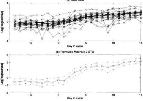
The progesterone data were collected in a study of early pregnancy loss conducted by the Institute for Toxicology and Environmental Health at the Reproductive Epi- demiology Section of the California Department of Health Services, Berkeley, USA. Figures 1.1 and 1.2 show levels of urinary metabolite progesterone over the course of the women’s menstrual cycles (days). The observations came from patients with healthy reproductive function enrolled in an artificial insemination clinic where insemination attempts were well-timed for each menstrual cycle. The data had been aligned by the day of ovulation (Day 0), determined by serum luteinizing hormone, and truncated at each end to present curves of equal length. Measurements were recorded once per day per cycle from 8 days before the day of ovulation and until 15 days after the ovulation. A woman may have one or several cycles. The length of the observation period is 24 days. Some measurements from some subjects were missing due to various reasons. The data set consists of two groups: the conceptive progesterone curves (22 menstrual cycles) and the nonconceptive progesterone curves (69 menstrual cycles). For more details about this data set, see Yen and Jaffe (1 99 I),

Brumback and Rice (1 998), and Fan and Zhang (2000), among others.

Figure 1.1 (a) presents a spaghetti plot for the 22 raw conceptive progesterone curves. Dots indicate the level of progesterone observed in each cycle, and are connected with straight line segments. The problem of missing values is not serious here because each cycle curve has at least 17 out of 24 measurements. Overall, the raw curves present a similar pattern: before the ovulation day (Day 0), the raw curves

(27)

MOTIVATING LONGITUDINAL DATA EXAMPLES 3

(a) Raw Data

I

i5

4 P 8 0 - -I -5 - 1 -5 0 5 10 15 Day in cycle (b) Pointwise Means i 2 STD 3 7 - r 1 +,-

,

- 't / r 1: - i - .. ,L7 G I 15 -21 . -5 0 5 10 Day in cycle

Fig. 7.7 The conceptive progesterone data.

are quite flat, but after the ovulation day, they generally move upward. However, it is easy to see that within a cycle curve, the measurements vary around some underlying curve which appears to be smooth, and for different cycles, the underlying smooth curves are different from each other. Figure 1.1 (b) presents the pointwise means (dot-dashed curve) with 95% pointwise standard deviation (SD) band (cross-dashed curves). They were obtained in a simple way: at each distinct design time point

t,

the mean and standard deviation were computed using the cross-sectional data at

t.

It can be seen that the pointwise mean curve is rather smooth, although it is not difficult to discover that there is still some noise appeared in the pointwise mean curve.

Figure 1.2 (a) presents a spaghetti plot for the 69 raw nonconceptive progesterone curves. Compared to the conceptive progesterone curves, these curves behave quite similarly before the day of ovulation, but generally show a different trend after the ovulation day. It is easy to see that, like the conceptive progesterone curves, the underlying individual cycles of the nonconceptive progesterone curves appear to be smooth, and so is their underlying mean curve. A naive estimate of the underlying mean curve is the pointwise mean curve, shown as dot-dashed curve in Figure 1.2 (b). The 95% pointwise SD band (cross-dashed curves) provides a rough estimate for the accuracy of the naive estimate.

The progesterone data have been used for illustrations of nonparametric regression methods by several authors. For example, Fan and Zhang (2000) used them to illustrate their two-step method for estimating the underlying mean function for longitudinal data or functional data, Brumback and Rice (1998) used them to illus-

(28)

4 INTRODUCTION

(b) Pointwise Means f 2 STD

f i g , f.2 The nonconceptive progesterone data.

trate a smoothing spline mixed-effects modeling technique for estimating both mean and individual functions, while Wu and Zhang (2002a) used them to illustrate a local polynomial mixed-effects modeling approach.

1.1.2 ACTG

388

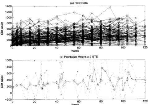
Data

The ACTG 388 data were collected in an AIDS clinical trial study conducted by the AIDS Clinical Trials Group (ACTG). This study randomized 5 17 HIV- 1 infected patients to three antiviral treatment arms. The data from one treatment arm will be used for illustration of the methodologies proposed in this book. This treatment arm includes 166 patients treated with highly active antiretroviral therapy (HAART) for 120 weeks during which CD4 cell counts were monitored at baseline and at weeks 4,

8, and every 8 weeks thereafter (up to 120 weeks). However, each individual patient might not exactly follow the designed schedule formeasurements, and missing clinical visits for CD4 cell measurements frequently occurred. CD4 cell count is an important marker for assessing immunologic response of an antiviral regimen. Of interest are CD4 cell count trajectories over the treatment period for individual patients and for the whole treatment arm. More details about this study and scientific findings can be found in Fischl et al. (2003) and Park and Wu (2005).

The CD4 cell count data from the 166 patients during 120 weeks of treatment are plotted in Figure 1.3 (a). From this spaghetti plot, it is difficult to capture any useful information. It can be seen that the individual CD4 cell counts are quite noisy

(29)

MOTIVATING LONGITUDINAL DATA EXAMPLES 5

over time. We usually expect that the CD4 cell counts would increase if the antiviral treatment was effective. But from this plot, it is not easy to see any patterns among the individual patients’ CD4 counts. Before a parametric model is found to fit this data set, we would have to assume that these individual curves are smooth but corrupted with noise.

(a) Raw Data

T---

,

I 4 O 0 1 - - -\, Week (b) Pointwise Means f 2 STD _ _ _ _ I looor --- -- I * x x , __-____ -1 A. 20 40 60 80 100 120 Week

Fig. 1.3 The ACTG 388 data.

Figure 1.3 (b) presents the simple pointwise means (solid curve with dots) of the CD4 counts and their 95% pointwise SD band (cross-dashed curves). This jiggly connected pointwise mean function shows an upward trend, but it is not smooth, although the underlying mean function appears to be smooth. Moreover, the pointwise SDs are not always computable, because at some design time points (e.g., the third design time point from the right end), only a single cross-sectional data point is available. In this case, the pointwise mean is just the cross-sectional measurement itself and the pointwise SD is 0, which is not a proper measure for the accuracy of the pointwise mean. In the plot, we replaced this 0 standard deviation by the estimated standard deviation b of the measurement errors, computed using all the residuals. However, this only partially solves the problem.

Without assuming parametric models for the mean and individual curves for the ACTG 388 data, nonparametric modeling techniques are then necessarily involved to handle the aforementioned problems. An example is provided by Park and Wu (2005), where they employed a kernel-based mixed-effects modeling approach.

(30)

6 INTRODUCTION

1.1.3 MACS

Data

Human immune-deficiency virus (HIV) destroys CD4 cells (T-lymphocytes, a vital component of the immune system) so that the number or percentage of CD4 cells in the blood of a patient will reduce after the subject is infected with HIV. The CD4 cell level is one of the important biomarkers to evaluate the disease progression of HIV infected subjects. To use the CD4 marker effectively in studies of new antiviral therapies or for monitoring the health status of individual subjects, it is important to build statistical models for CD4 cell count or percentage. For CD4 cell count, Lange et al. (1992) proposed Bayesian models while Zeger and Diggle (1 994) employed a semiparametric model, fitted by a backfitting algorithm. For further related references, see Lange et a]. (1992).

A subset of HIV monitoring data from the Multi-center AIDS Cohort Study (MACS) contains the HIV status of 283 homosexual men who were infected with HIV during the follow-up period between 1984 and 199 1. Kaslow et al. (1987) presented the details for the related design, methods and medical implications of this study. The response variable is the CD4 cell percentage of a subject at a number of design time points after HIV infection. Three covariates were assessed in this study. The first one, “Smoking”, takes the values of 1 or 0, according to whether a subject is a smoker or nonsmoker, respectively. The second covariate, “Age”, is the age of a subject at the time of HIV infection. The third covariate, “PreCDP, is the last measured CD4 cell percentage level prior to HIV infection. All three covariates are time-independent and subject-specific. All subjects were scheduled to have clinical visits semi-annually for taking the measurements of CD4 cell percentage and other clinical status, but many subjects frequently missed their scheduled visits which re- sulted in unequal numbers of measurements and different measurement time points from different subjects in this longitudinal data set. We plotted the raw data from individual subjects and the simple pointwise mean of the data in Figure 1.4.

The aim of this study is to assess the effects of cigarette smoking, age at sero- conversion and baseline CD4 cell percentage on the CD4 cell percentage depletion after HIV infection among the homosexual men population. From Figure 1.4, we can see that there was a trend of CD4 cell percentage depletion although the pointwise mean curve does not provide a good smooth estimate for this trend. Thus, a nonparametric modeling approach is required to characterize the CD4 cell depletion trend and to correlate this trend to the aforementioned covariates. In fact, Zeger and Diggle (1994), Wu and Chiang (2000), Fan and Zhang (2000), Rice and Wu (2001), Huang, Wu and Zhou (2002), among others have applied various nonparametric regression methods including time varying coefficient models to this data set. Similarly, we will use this data set to illustrate the proposed nonparametric regression models and smoothing methods in the succeeding chapters.

(31)

MIXED-EFFECTS MODELING: FROM PARAMETRIC TONONPARAMETRIC 7

fa) Raw Data

0 1 2 3 4 5 6 Time fb) Poinhvise Means

*

2 STD 4 2 3 4 5 6 0 ₁ lo

1

0 Time

Fig, 1.4 The MACS data.

1.2 MIXED-EFFECTS MODELING: FROM PARAMETRIC TO NONPARAMETRIC

1.2.1 Parametric Mixed-Effects Models

For modeling longitudinal data, parametric mixed-effects models, such as linear and nonlinear mixed-effects models, are a natural tool. Linear or nonlinear mixed-effects models can be specified as hierarchical linear and nonlinear models from a Bayesian perspective.

Linear mixed-effects (LME) models are used when the relationship between a longitudinal response variable and its covariates can be expressed via a linear model. The LME model introduced by Harville (1976, 1977), and Laird and Ware (1982) can be generally written as

where yi and ~i are, respectively, the vectors of responses and measurement errors for the i-th subject,

p

and bi are, respectively, the vectors of fixed-effects (population parameters) and random-effects (individual parameters), and

X

i and Zi are the associated fixed-effects and random-effects design matrices. It is easy to notice that the mean and covariance matrix of yi are given by

(32)

8 INTRODUCTION

Nonlinear mixed-effects (NLME) models are used when the relationship between a longitudinal response variable and its covariates can be expressed via a nonlinear model, which is known except for some parameters. A general hierarchical nonlinear model or NLME model may be written as (Davidian and Giltinan 1995, Vonesh and Chinchilli 1996):

(1 .2)

Yi

= f(Xi,Pi)

+

ei,

Pi

= d(Ai,Bi,P,bi),

bi N(O,D), ~i N(O,Ri), i = 1,2;-.,n,

where f(Xi,

pi)

= [f(xil

,Pi),

. . . ,

f(xini,

Pi)]T

with f ( - ) beinga known function,

Xi = [ x i l , .

. . ,

xinilT a design matrix and

Pi

a subject-specific parameter for the

i-th subject. In the above NLME model, the d(.) is a known function of the design matrices Ai and Bi, the fixed-effects vector

p

and the random-effects vector b i. As

an example, a simple linear model for

p i

can be written as

Pi

= AiP

+

Bibi,

i

= 1,2, . . .

,

n. The marginal mean and variance-covariance of y i cannot be given for a general NLME model. They may be approximated using linearization techniques (Sheiner, Rosenberg and Melmon 1972, Sheiner and Beal 1982, and Lindstrom and Bates 1990, among others).

More detailed definitions ofthe LME and NLME models will be given in Chapter 2 .

In either a LME model or a NLME model, the between-subject and within-subject variations are separately quantified by the variance components

D

and Ri, _i=

1: 2, .

.

,

n. In a longitudinal study, the data from different subjects are usually assumed to be independent, but the data from the same subject may be correlated. The correlations may be caused by the between-subject variation (heterogeneity across subjects) andor the serially correlated measurement error. Ignoring the existing correlation of longitudinal data may lead to incorrect and inefficient inferences. Thus, a key requirement for longitudinal data analysis is to appropriately model and accu- rately estimate the variance components so that the underlying mean and individual functions can be efficiently modeled. This is the reason why longitudinal data analysis is more challenging in both theoretical development and practical implementation compared to cross-sectional data analysis.

The successful application of a LME or a NLME model to longitudinal data analysis strongly depends on the assumption of a proper linear or nonlinear model for the relationship between the response variable and the covariates. Sometimes this assumption may be invalid for a given longitudinal data set. In this case, the relationship between the response variable and the covariates has to be modeled nonparametri- cally. Therefore, we need to extend parametric mixed-effects models to nonparametric mixed-effects models.

1.2.2 Nonparametric Regression and Smoothing

A parametric regression model requires an assumption that the form of the underlying regression hnction is known except for the values of a finite number of parameters. The selection of a parametric model depends very much on the problem at hand. Sometimes the parametric model can be derived from mechanistic theories behind the scientific problem, whereas at other times the model is based on experience or

(33)

MIXED-EFFECTS MODELING: FROM PARAMETRIC TONONPARAMETRIC 9

is simply deduced from scatter plots of the data. A serious drawback of parametric modeling is that a parametric model may be too restrictive in some applications. If an inappropriate parametric model is used, it is possible to produce misleading conclusions from the regression analysis. In other situations, a parametric model may not be available to use. To overcome the difficulty caused by the restrictive assumption of a parametric form of the regression function, one may remove the restriction that the regression function belongs to a parametric family. This approach leads to so-called nonparametric regression.

There exist many nonparametric regression and smoothing methods. The most popular methods include kernel smoothing, local polynomial fitting, regression @oly- nomial) splines, smoothing splines, and penalized splines. Some other approaches such as locally weighted scatter plot smoothing (LOWESS), wavelet-based methods and other orthogonal series-based approaches are also frequently used in practice. The basic idea of these nonparametric approaches is to let the data determine the most suitable form of the functions. There are one or two so-called smoothing parameters in each of these methods for controlling the model complexity and the trade-off between the bias and variance of the estimator. For example, the bandwidth h in local kernel smoothing determines the smoothness of the regression function and the goodness-of-fit of the model to the data so that when h = 00, the local nonparametric

model becomes a global parametric model; whereas when h = 0, the resulting estimate essentially interpolates the data points. Thus, the boundary between parametric and nonparametric modeling may not be clear-cut if one takes the smoothing parameter into account. Nonparametric and parametric regression methods should not be regarded as competitors, instead they complement each other. In some situations, nonparametric techniques can be used to validate or suggest a parametric model. A

combination of both nonparametric and parametric methods is more powerful than any single method in many practical applications.

There exists a vast literature on smoothing and nonparametric regression methods for cross-sectional data. Good surveys on these methods can be found in books by de Boor (1978), Eubank (1988), H ardle (1990), Wahba (l990), Green and Silverman (1994), Wand and Jones (1993, Fan and Gijbels (1 996), and Ruppert, Wand and Carroll (2003), among others. However, very little effort has been made to develop nonparametric regression methods for longitudinal data analysis until recent years. Miiller (1988) was the first to address longitudinal data analysis using nonparametric regression methods. However, in this earlier monograph, the basic approach is to estimate each individual curve separately, thus, the within-subject correlation of the longitudinal data was not considered in modeling. The methodologies in M iiller

(1 988) are essentially similar to the nonparametric regression methods for cross- sectional data.

In recent years, there has been a boom in the development of nonparametric regression methods for longitudinal data analysis which include utilization of kernel-type smoothing methods (Hoover et al. 1998, Wu and Chiang 2000, Wu, Chiang and Hoover 1998, Fan and Zhang 2000, Lin and Carroll 200 1 a, b, Wu and Zhang 2002a. Welsh, Lin and Carroll 2002, Cai, Li and Wu 2003, Wang 2003, Wang, Carroll and Lin 2005), smoothing spline methods (Brumback and Rice 1998, Wang 1998a, b,

(34)

I 0 INTRODUCTION

Zhang et al. 1998, Lin and Zhang 1999, Guo 2002a, b) and regression (polynomial) spline methods (Shi, Weiss and Taylor 1996, Rice and Wu 200 1, Huang, Wu and Zhou 2002, Wu and Zhang 2002b, Liang, Wu and Carroll 2003). There is a vast amount of recent literature in this research area, and it is impossible for us to have an exhaustive list here. The importance of nonparametric modeling methods has been recognized in longitudinal data analysis and for practical applications, since nonparametric methods are flexible and robust against parametric assumptions. Such flexibility is useful for exploration and analysis of longitudinal data, when appropriate parametric models are unavailable. In this book, we do not intend to cover all nonparametric regression techniques. Instead we will focus on the most popular methods such as local polynomial smoothing, regression (polynomial) splines, smoothing splines and penalized splines (P-Splines) approaches. We incorporate these nonparametric smoothing pro- cedures into mixed-effects models to propose nonparametric mixed-effects modeling techniques for longitudinal data analysis.

1.2.3 Nonparametric Mixed-Effects Models

A longitudinal data set such as the progesterone data and the ACTG 388 data presented in Section 1.1, can be expressed in a common form as

where t i j denote the design time points (e.g., “day” in the progesterone data), y i j the

responses observed at t i j (e.g. “log(Progesterone)” in the progesterone data), n i the number of observations for the i-th subject, and n is the number of subjects.

For such a longitudinal data set, we do not assume a parametric model for the relationship between the response variable and the covariate time. Instead, we just assume that the individual and the population mean functions are smooth functions of time

t,

and let the data themselves determine the form ofthe underlying functions. Following Wu and Zhang (2002a), we introduce a nonparametric mixed-effects (NPME) model as

& ( t )

= q ( t ) + V i ( t ) + € i ( t ) ,

i

= 1 , 2 , - . . , n , (1.4)

where q ( t ) models the population mean function of the longitudinal data set, called fixed-effect function, vi(t) models the departure of the i-th individual function from the population mean function

~ ( t ) ,

called the i-th random-effect function, and c i ( t )

the measurement errors that can not be explained by both the fixed-effect and the random-effect functions.

It is generally assumed that vi(t), _i= 1,2,.

.

. ~ R are i.i.d realizations ofan under-

lyingsmoothprocess(SP),v(t), withmean function0andcovariance function y(s,

t ) ,

and

~ i ( t )

are i.i.d realizations ofan uncorrelated white noise process,

~ ( t ) ,

with mean function 0 and variance function y f ( s , t ) = ~ ~ ( t ) l { , = ~ j . That is, v ( t )

-

SP(0,y) and

~ ( t )

-

SP(0, _ye).Here y(s,

t )

quantifies the bctween-subject variation while the

~ ‘ ( t )

quantifies the within-subject variation. When discussing the likelihood-based inferences or Bayesian interpretation, for simplicity, we generally assume that the associated processes are Gaussian, i.e., v ( t )

-

GP(0, y), and t

-

GP(0, y6).

(35)

SCOPE OF THE BOOK I 1

Under the NPME modeling framework, we need to accomplish the following tasks: (1) to estimate the fixed-effect (population mean) function

~ ( t ) ;

(2) to predict the random-effect functions vi(t) and individual functions s i ( t ) =

~ ( t )

+

vi(t), i = 1,2, .

. . ,

n; (3) to estimate the covariance function y(s,

t ) ;

and (4) to estimate the noise variance function

a'(t).

The

~ ( t ) ,

y(s, t ) and

~ ' ( t )

characterize the population features of a longitudinal response while

vi(t)

and s i ( t ) capture the individual features. For simplicity, the population mean function

~ ( t )

and the individual functions

s i ( t )

are sometimes re- ferred to as population and individual curves, respectively. Because in the NPME model (1.4), the target quantities

~ ( t ) ,

v i ( t ) , y(s,

t )

and

a2(t)

are all nonparametric, the combination of smoothing techniques and mixed-effects modeling approaches is necessary for estimating these unknown quantities. We will also extend this NPME modeling idea to semiparametric models, time varying coefficient models and models for analyzing discrete longitudinal data.

1.3

SCOPE

OF THE

BOOK

For longitudinal data analysis, a simple strategy is the so-called two-stage or derived variable approach (Diggle et al. 2002). The first step is to reduce the repeated measurements from individual subjects or units into one or two summary statistics, and the second step is to conduct the analysis for the summarized variables. This method may not be efficient if the repeatedly measured variables change significantly and informatively over time. In the book by Diggle et al. (2002), three alternative modeling strategies are discussed, i.e., the marginal modeling analysis, the random-effects modeling approach, and the transition modeling approach. For all three approaches, the dependence of the response on the explanatory variables and the autocorrelation among the responses are considered. In this book, the ideas from the three strategies will be used under the framework of nonparametric regression techniques although we may not explicitly use the same wording.

It is impossible to exhaustively survey all the nonparametric smoothing and regression methods for longitudinal data analysis in this monograph. Selection of covered materials is based on our experiences with practical data problems. We emphasize the introduction of basic ideas of methodologies and their applications to data analysis throughout the book. Since this book is an extension of nonparametric smoothing and regression methods for longitudinal data analysis, it is essential to combine the techniques from these two areas in an efficient way.

1.3.1

The building blocks of the NPME models include parametric mixed-effects models and nonparametric smoothing techniques. To better understand NPME models we begin with a review of LME and nonparametric smoothing techniques.

Two most popularparametric mixed-effects models are linear mixed-effects (LME) and nonlinear mixed-effects (NLME) models. LME models are the simplest mixed-

(36)

12 INJRODUC JlON

effects models in which the responses are linear functions of the fixed-effects and random-effects. In Chapter 2, we shall briefly discuss how the models are specified, how the parameters are estimated and how the variance components are estimated. In particular, we briefly mention random-coefficients models as special cases of the usual LME models. In Chapter 2, we will also briefly review NLME models and related inference methods. In a NLME model, the responses are nonlinear functions of the fixed-effects and random-effects. It is a challenging task to estimate the parameters in NLME models. We will summarize the two-stage, first order approximation and conditional first order approximation methods in this chapter. Generalized linear and nonlinear mixed-effects models will also be briefly discussed.

In Chapter 3, we shall review some popular nonparametric regression techniques that include local polynomial smoothing, regression splines, smoothing splines, and penalized splines, among others. We will briefly discuss the basic ideas of these techniques, computational issues and smoothing parameter selections.

1.3.2

Fundamental Development

of

the

NPME

Models

Fundamental developments of the NPME modeling techniques will be presented in Chapters 4-7, and each chapter covers one popular nonparametric method. These are the core contents of this book and lay a good foundation for further extensions of the NPME models. Each of these chapters will also provide a review for the nonparametric population mean (NPM) model and naive smoothing methods before the mixed-effects modeling approach is introduced.

In Chapter 4, we will mainly investigate local polynomial mixed-effects models after a review of the NPM model and the local polynomial kernel-based generalized estimating equations (LPK-GEE) methods. The local polynomial smoothing approaches and LME modeling techniques are combined to estimate unknown functions and parameters for the NPME model (1.4). The key idea for this method is that for each fixed time point t ,

v(t)

and vi(t) in the NPME model (1.4) are approximated by a polynomial of some degree so that a local LME model is formed and solved. We will also study the bandwidth selection methods. Some theoretic results will be presented to provide theoretical justifications for the proposed methodologies. One of the advantages of this approach is that at each time point

t ,

the associated local LME model can be solved by the existing statistical software such as the h e function in S-PLUS, or the procedure PROC MIXED in SAS.

In Chapter 5, we will introduce regression spline mixed-effects models. The main idea is to approximate

~ ( t )

and u i ( t ) by regression splines so that the NPME model (1.4) can be transformed into a global parametric model, which can be solved using the existing statistical software such as S-PLUS or SAS. However, one needs to locate the knots for the regression splines and choose the number ofknots using some model selection rules. The regression spline method is simple to implement and easy to understand. That is why it is the first NPME modeling technique studied in the literature (Shi, Weiss and Taylor 1996) and it is also attractive to practitioners.

In Chapter 6, we will focus on smoothing spline mixed-effects modeling techniques. The smoothing spline approach is one of the major nonparametric smoothing

(37)

SCOPE OF THE BOOK 13

methods and has been well developed for cross-section i.i.d. data. For longitudinal data, several authors (Wang 1998a, Brumback and Rice 1998, Guo 2002a) have proposed some techniques using the LME model representation of a smoothing spline. Our idea is to incorporate the roughness of

~ ( t )

and v i ( t ) of the NPME model (1.4)

into NPME modeling in a natural way, and to develop new techniques for variance component estimation and smoothing parameter selection.

The penalized spline (P-spline) method recently became very popular in nonparametric modeling since it is computationally easier than the smoothing spline method, but still inherits all the advantages of the smoothing spline approach. We will combine the mixed-effects modeling ideas and the P-spline techniques for longitudinal data analysis in Chapter 7.

1.3.3 Further Extensions

of

the NPME Models

The fundamental NPME modeling methodologies introduced in Chapters 4-7 can be extended to semiparametric and varying-coefficient models. In a semiparametric mixed-effects model, part of the variations in the response variable can be explained by given parametric models of some covariates in the fixed effect component andor the random-effect component, while the remaining is explained by a nonparametric function of time. In a time varying coefficient mixed-effects model, the coefficients of the fixed-effects and random-effects covariates are smooth functions of time. These two kinds of models are very important and useful in practical longitudinal data analysis. The challenging question is how to estimate the constant and time-varying parameters under a mixed-effects modeling framework. The fundamental NPME modeling methodologies can also be extended to discrete longitudinal data analysis. Chapters 8-10 will cover these extended models in details.

Chapter 8 will focus on semiparametric models for longitudinal data. In this chapter, we first provide a review of semiparametric population mean models before the semiparametric mixed-effects models are introduced. The local polynomial smoothing, regression spline, penalized spline, and smoothing spline methods will be covered. The methods that do not involve smoothing are also briefly discussed. The more sophisticated semiparametric nonlinear mixed-effects models will be presented. In Chapter 9, we will introduce time varying coefficient models for longitudinal data. First the time varying coefficient nonparametric population mean (TVC-NPM) models are reviewed. The local polynomial smoothing, regression spline, penalized spline, and smoothing spline methods are introduced to fit the TVC-NPM models. The smoothingparameter selections are discussed and a backfitting algorithm is proposed. The two-step method of Fan and Zhang (2000) is also adapted to fit the TVC-NPM models. The TVC-NPM models with time-independent covariates are briefly discussed. The extension of the TVC-NPM models that include both parametric (linear or nonlinear) and nonparametric time varying coefficients is briefly explored. The time varying coefficient nonparametric mixed-effects (TVC-NPME) models, which is the focus of this chapter, are investigated in details. The aforementioned smoothing approaches are developed to fit the TVC-NPME models. The semiparametric

(38)

14 /NTRODUCT/ON

TVC-NPME models that include both constant and time varying coefficients are also introduced.

Chapter 10 will concentrate on an introduction to nonparametric regression methods for discrete longitudinal data. We first review the LPK-GEE methods for the generalized nonparametric and semiparametric population mean models proposed by Lin and Carroll (2000, 2001a,b), Wang (2003), Wang, Carroll and Lin (2005).

We then introduce the generalized nonparametric mixed-effects models and generalized time varying coefficient nonparametric mixed-effects models as well as the local polynomial approach for fitting these models in details. The asymptotic properties of the estimators are also investigated. Finally the generalized semiparametric additive mixed-effects models initiated by Lin and Zhang (1999) are introduced in detail.

1.4 IMPLEMENTATION OF METHODOLOGIES

Most methodologies introduced in this book can be implemented using existing software such as S-PLUS and SAS, among others, although it may be more efficient to use Fortran, C or MATLAB codes. The latter usually requires intensive programming since Fortran, C or MATLAB subroutines for parametric mixed-effects modeling or nonparametric smoothing techniques are unavailable. We shall publish our MAT- LAB codes for most of the methodologies proposed in this book and the data analysis examples on our website: http://www. urmc.rochester:edu/smd/biostat/people/faculty /WuSile/publications.htm and keep updating the codes when it is necessary. We shall also make the data sets used in this book available through our website.

1.5 OPTIONS FOR READING THIS BOOK

Readers who are particularly interested in one or two of the nonparametric smoothing techniques for longitudinal data analysis may select the relevant chapters to read. For a lower level graduate course, Chapters 1-7 are recommended. If students already have some background in mixed-effects models and nonparametric smoothing techniques, Chapters 2 and 3 may be briefly reviewed or even skipped. Chapters 8-10 may be included in a higher level graduate course or can be used as individual research materials for those who may want to do research in this area.

1.6 BIBLIOGRAPHICAL NOTES

Nonparametric regression methods for longitudinal data analysis is still an active research area. In this book, we have not attempted to provide an exhaustive review of all the methodologies in the literature. Interested readers are strongly advised to read additional work by other authors whose methodologies have not been covered in this

book. For nonparametric estimation of individual curves of longitudinal data without a mixed-effects framework, we refer readers to M iiller (1 988), and for nonparametric

(39)

BlBLlOGRAPHlCAL NOTES 15

techniques for analyzing functional data (which may be regarded as longitudinal data with a very large number of measurements per subject), we refer readers to Ram- say and Silverman (1997,2002). Important references for parametric mixed-effects modeling methods, nonparametric smoothing techniques and various nonparametric and semiparametric models are provided at the end of this book. Below, we briefly mention some important monographs on these subjects.

Various models and methods for dealing with longitudinal data analysis are given by Diggle, Liang and Zeger (1 994), and Diggle, Heagerty, Liang and Zeger (2002). Monographs on linear and nonlinear mixed-effects models include Lindstrom and Bates (1990), Lindsey (1993), Davdian and Giltinan (1995), Vonesh and Chinchilli (1 996), and Verbeke and Molenberghs (2000), among others. Longford (1 993) surveys methods on random coefficient models for longitudinal data. Jones (1 993) treats longitudinal data with serial correlation using a state-space approach. Pinheiro and Bates (2000) discuss the implementation of mixed-effects modeling in S and S-PLUS. Methods on variance components estimation are surveyed by Searle, Casella and Mc- Culloch (l992), and by Cox and Solomon (2003). A recent monograph on theories and applications of mixed models is given by Demidenko (2004).

A good survey on kernel smoothing is provided by Wand and Jones (1 995). A very readable introduction to local polynomial modeling and its applications is given by Fan and Gijbels (1 996). A classical introduction to B-splines is given by de Boor (1 978). Penalized splines and their applications in semiparametric models are investigated by Ruppert, Wand and Carroll (2003). Wahba (1990) and Green and Silverman (1994) are two monographs on smoothing spline approaches to nonparametric regression. Various nonparametric smoothing techniques and their applications can be found in books by Eubank (1 988, 1999), H ardle (1 990), Simonoff (1 996), and Efromovich (1 999), among others. Nonparametric lack-of-fit testing techniques are discussed by Hart (1997).

Generalized linear models are explored by McCullagh and Nelder (1 989). Recent advances on theories and applications of semiparametric models for independent data are surveyed by H ardle, Liang and Gao (2000). Ruppert, Wand and Carroll (2003) survey methods for fitting semiparametric models using P-splines.

(40)

(41)

2

~

Parametric Mixed- Efec ts

Models

2.1 INTRODUCTION

Parametric mixed-effects models or random-effects models are powerful tools for longitudinal data analysis. Linear and nonlinear mixed-effects models (including generalized linear and nonlinear mixed-effects models) have been widely used in many longitudinal studies. Good surveys on these approaches can be found in the books by Searle, Casella, and McCulloch (1 992), Davidian and Giltinan (1995),

Vonesh and Chinchilli (1996), Verbeke and Molenberghs (2000), Pinheiro and Bates

(2000), Diggle et al. (2002), and Demidenko (2004), amongothers. In this chapter, we shall review various parametric mixed-effects models and emphasize the methods that w