A Comparison of Machine Learning and Traditional Demand Forecasting Methods

(1)

Clemson University Clemson University

TigerPrints

All Theses Theses

August 2020

A Comparison of Machine Learning and Traditional Demand

Forecasting Methods

Franz Stoll

Clemson University, [email protected]

Follow this and additional works at: https://tigerprints.clemson.edu/all_theses Recommended Citation

Recommended Citation

Stoll, Franz, "A Comparison of Machine Learning and Traditional Demand Forecasting Methods" (2020). All Theses. 3367.

https://tigerprints.clemson.edu/all_theses/3367

This Thesis is brought to you for free and open access by the Theses at TigerPrints. It has been accepted for inclusion in All Theses by an authorized administrator of TigerPrints. For more information, please contact

(2)

A COMPARISON OF MACHINE LEARNING AND TRADITIONAL

DEMAND FORECASTING METHODS

A Thesis Presented to the Graduate School of

Clemson University

In Partial Fulfillment of the Requirements for the Degree

Master of Science Industrial Engineering

by

Franz Carlos Stoll Quevedo August 2020

Accepted by:

Dr. Scott J. Mason, Committee Chair Dr. William G. Ferrell

(3)

ABSTRACT

Obtaining accurate forecasts has been a challenging task to achieve for many organizations, both public and private. Today, many firms choose to share their internal information with supply chain partners to increase planning efficiency and accuracy in the hopes of making appropriate critical decisions. However, forecast errors can still increase costs and reduce profits. As company datasets likely contain both trend and seasonal behavior, this motivates the need for computational resources to find the best parameters to use when forecasting their data. In this thesis, two industrial datasets are examined using both traditional and machine learning (ML) forecasting methods. The traditional methods considered are moving average, exponential smoothing, and autoregressive integrated moving average (ARIMA) models, while K-nearest neighbor, random forests, and neural networks were the ML techniques explored. Experimental results confirm the importance of performing a parametric grid search when using any forecasting method, as the output of this process directly determines the effectiveness of each model. In general, ML models are shown to be powerful tools for analyzing industrial datasets.

(4)

TABLE OF CONTENTS

ABSTRACT ... ii

LIST OF FIGURES ... v

LIST OF TABLES ... vii

INTRODUCTION ... 1

CHAPTER ONE: LITERATURE REVIEW ... 2

1.1. Demand Forecasting ... 4

1.2. Data Mining ... 5

1.3. Forecasting Methods ... 6

1.3.1. Moving Average (MA) ... 7

1.3.2. Exponential Smoothing (ES) ... 7

1.3.3. Auto-Regressive Integrated Moving Average (ARIMA) ... 9

1.4. Machine Learning ... 10

1.4.1. K-Nearest Neighbor (K-NN) Regression ... 11

1.4.2. Ensembles of Decision Trees (Random Forests) ... 12

1.4.3. Neural Networks models (NN) Models (Deep Learning) ... 13

CHAPTER TWO: DATASETS AND METHODOLOGY ... 15

2.1. Dataset 1: Office Supplies ... 15

2.1.1. Analysis for SKU Marker ABC... 16

2.1.2. Traditional Forecasting Models for Marker ABC ... 18

2.1.2.1. Moving Average (MA) ... 18

2.1.2.2. Simple Exponential Smoothing (SES) ... 20

2.1.2.3. Double Exponential Smoothing (DES) ... 21

2.1.2.4. Triple Exponential Smoothing (TES) ... 22

2.1.2.5. ARIMA ... 24

2.1.3. Machine Learning Forecasting Models for SKU Marker ABC ... 26

2.1.3.1. K-Nearest Neighbors (KNN) ... 26

2.1.3.2. Decision Tree ... 27

2.1.3.3. Ensembles of Decision Trees (Random Forests) ... 29

2.1.3.4. Recurrent Neural Network ... 30

(5)

2.1.5. Traditional Forecasting Models for SKU Ballpoint Pen XYZ ... 34

2.1.5.1. Moving Average ... 34

2.1.5.2. Simple Exponential Smoothing ... 35

2.1.5.5. ARIMA model ... 39

2.1.6. Machine Learning Forecasting Models for SKU Ballpoint Pen XYZ ... 40

2.1.6.2. Decision Tree (DT) ... 41

2.1.6.3. Ensembles of Decision Trees (Random Forests) ... 43

2.1.7. Preliminary Results Discussion for Office Supplies Datasets ... 46

2.2. Dataset 2: Food Prices ... 50

2.2.1. Dataset Description and Research Overview ... 50

2.2.2. Traditional Forecasting Models for Product_1359 ... 53

2.2.2.1. Moving Average (MA) ... 53

2.2.2.2. Simple Exponential Smoothing (SES) ... 55

2.2.2.5. ARIMA ... 58

2.2.3. Machine Learning Forecasting Models ... 59

2.2.3.2. Decision Tree (DT) ... 61

2.2.3.3. Ensembles of Decision Tree (Random Forests) ... 62

2.2.4. Preliminary Results Discussion for Food Prices Datasets ... 64

CHAPTER THREE: CONCLUSIONS AND FUTURE RESEARCH ... 66

3.1 Summary of Research Conclusions ... 67

3.2 Summary of Future Recommendations ... 67

(6)

LIST OF FIGURES

Figure 1: Evolution of supply chain management (Adapted from Ballou, 2007) ... 3

Figure 2: Process of forecasting (Adapted from Brown et al., 2013) ... 5

Figure 3: Trade-off Model Training and Test accuracy (Adapted from Müller and Guido, 2016) 11 Figure 4: Examples of predictions using different values of neighbors (Adapted from Müller and Guido, 2016) ... 11

Figure 5: Examples of predictions using different values of neighbors (Adapted from Müller and Guido, 2016) ... 12

Figure 6: Random forest structure (Adapted from Breiman, 2001) ... 13

Figure 7: Single hidden layer Neural Network (Adapted from Müller and Guido, 2016) ... 13

Figure 8: 30 years forecasting using 6 hidden layers (Adapted from Hyndman and Athanasopoulos, 2018) ... 14

Figure 9: Distribution of Products ... 15

Figure 10: Quantity Distribution of production quantity based on family’s product ... 16

Figure 11: Pareto Principle for Marker ABC group ... 17

Figure 12: Time Series Production per week for Marker ABC ... 17

Figure 13: Probability density for daily production for Marker ABC ... 18

Figure 14: Output for different levels of Moving Average (order 2, 5, 7, 10) ... 19

Figure 15: MAPE and RMSE Error vs MA Order level ... 20

Figure 16: RMSE behavior using different alpha levels ... 20

Figure 17: Simple Exponential Smoothing plot with different α values ... 21

Figure 18: RMSE behavior for different combination of alpha and beta ... 21

Figure 19: Double Exponential Smoothing plot using best α and ß values ... 22

Figure 20: RMSE behavior for different combinations of alpha, beta, and gamma ... 23

Figure 21: Triple Exponential Smoothing (Multiplicative Method) ... 23

Figure 22: Decomposition of Trend and Seasonal feature for Marker ABC ... 24

Figure 23: Diagnostics for ARIMA model ... 25

Figure 24: ARIMA (1, 0, 1) (0, 1, 1, 12) model for fitting Marker ABC data set ... 26

Figure 25: RMSE Error vs Number of neighbors using different training percentage ... 27

Figure 26: KNN – Modeling of Training data vs Forecast data ... 27

Figure 27: Decision Tree – Modeling of Training data vs depth of tree ... 28

Figure 28: Decision Tree – Modeling of Training data vs Forecast data ... 29

Figure 29: Ensembles of Decision Tree – Modeling of Training data vs numbers of trees ... 29

Figure 30: Ensembles of Decision Tree – Modeling of Training data vs Forecast data... 30

Figure 31: Comparison of different training levels vs model's RMSE using different layers ... 30

Figure 32: LSTM loss / error versus number of epochs used ... 31

Figure 33: RNN – LSTM model-s behavior of data analyzed... 31

Figure 34: Pareto Principle for Ballpoint Pen XYZ colors ... 32

Figure 35: Time Series Production per day for Ballpoint Pen XYZ color blue, red, and black ... 33

Figure 36: Probability density for weekly production for Ballpoint Pen XYZ color blue, red, and black ... 34

(7)

Figure 40: Best fit for Exponential Smoothing - All Color analyzed ... 36

Figure 41: RMSE behavior using different alpha and beta levels ... 37

Figure 42: Best fit for Double Exponential Smoothing - All Color analyzed ... 38

Figure 43: RMSE behavior using different alpha, beta, and gamma levels ... 39

Figure 44: Best fit for Triple Exponential Smoothing - All Color analyzed ... 39

Figure 45: AIC values for different combination of p, d, q for all color analyzed ... 40

Figure 46: ARIMA forecast test for 15 days ... 40

Figure 47: KNN Model testing different training sets and number of neighbors ... 41

Figure 48: KNN forecast testing ... 41

Figure 49: Decision Tree Model testing different training sets and depths ... 42

Figure 50: Decision Tree forecast testing ... 43

Figure 51: Random Forest Model testing different training sets and # of trees ... 44

Figure 52: Random Forest forecast testing ... 44

Figure 53: Trade-off between training and testing set using different Network combination ... 45

Figure 54: RNN – LSTM model-s behavior of data analyzed... 45

Figure 55: RMSE and MAPE comparison of forecasting techniques analyzed for Marker ABC . 47 Figure 56: RMSE and MAPE comparison of forecasting techniques analyzed for Ballpoint Pen XYZ ... 48

Figure 57: Distribution of demand orders per warehouses ... 51

Figure 58: Demand per category (left) and per product (right) for Warehouse Whse_J ... 51

Figure 59: Average price trend over time (2015-2018) ... 53

Figure 60: Average price distribution per region ... 52

Figure 61: Volume distribution between STD and Non-STD ... 53

Figure 62: Output for different levels of Moving Average (order 2, 5, 7, 10) ... 54

Figure 65: Simple Exponential Smoothing plot with different α values ... 55

Figure 66: RMSE behavior for different combination of alpha and beta ... 56

Figure 67: Double Exponential Smoothing plot using best α and ß values ... 57

Figure 68: RMSE behavior for different combinations of alpha, beta, and gamma ... 58

Figure 69: Triple Exponential Smoothing (Multiplicative Method) ... 58

Figure 70: AIC values for different combination of p, d, q for all color analyzed ... 59

Figure 71: ARIMA model fit for whole dataset (right) and testing values (left)... 59

Figure 72: Correlation between Average Price (target column) against data features ... 60

Figure 73: KNN Sensitivity analysis (top) and KNN data fit (bottom) ... 61

Figure 74: Sensitivity analysis (top) and DT data fit (bottom) ... 62

Figure 75: Sensitivity analysis (top) and RF data fit (bottom) ... 63

Figure 76: RNN Sensitivity analysis (top and middle) and RNN fitting (bottom) ... 64

(8)

LIST OF TABLES

Table 1: Supply chain risks and their drivers (Adapted from Chopra and Sodhi, 2004)... 4

Table 2: Distribution Summary for Marker ABC ... 18

Table 3: Error Summary for Moving Average Models ... 19

Table 4: Error Summary for Simple Exponential Smoothing - Marker ABC ... 20

Table 5: Error Summary for Double Exponential Smoothing - Marker ABC ... 21

Table 6: Error Summary for Triple Exponential Smoothing - Marker ABC ... 23

Table 7: Error summary for ARIMA model ... 25

Table 8: Error summary for KNN 86% Training data and neighbors=6 ... 27

Table 9: Breaking down of time series dates into features ... 28

Table 10: Error summary for Decision Tree 65% Training data and depth =2 ... 29

Table 11: Error summary for Ensembles Decision Tree 85% Training data and number of trees = 20 ... 30

Table 12: Error Summary for RNN – LSTM model for Marker ABC ... 31

Table 13: Distribution Summary per color ... 33

Table 15: Error Summary for Simple Exponential Smoothing – Ballpoint Pen XYZ ... 36

Table 16: Error Summary for Double Exponential Smoothing – Ballpoint Pen XYZ ... 37

Table 17: Error Summary for Triple Exponential Smoothing – Ballpoint Pen XYZ ... 38

Table 18: Error Summary for ARIMA – Ballpoint Pen XYZ ... 40

Table 19: Error summary for KNN – Ballpoint Pen XYZ ... 41

Table 20: Error summary for Decision Tree ... 42

Table 21: Error summary for Ensembles of Decision Trees (Random Forests) ... 43

Table 22: Error summary for Recurrent Neural Network ... 45

Table 23: Comparison between Traditional Methods and Machine Learning methods for Marker ABC ... 46

Table 24: Comparison table between Traditional Methods and Machine Learning methods for Ballpoint Pen XYZ ... 49

Table 25: Food Products Summary ... 50

Table 27: Error Summary for Simple Exponential Smoothing - ... 55

Table 28: Error Summary for Double Exponential Smoothing – Ballpoint Pen XYZ ... 56

Table 29: Error Summary for Triple Exponential Smoothing ... 57

Table 30: Error summary for ARIMA model ... 59

Table 31: Error summary for KNN ... 60

Table 32: Error summary for KNN ... 61

Table 33: Error summary for Ensembles of Decision Trees (Random Forests) ... 62

Table 34: Error summary for Recurrent Neural Network ... 63

Table 35: Comparison between Traditional Methods and Machine Learning methods for Marker ABC ... 64

(9)

INTRODUCTION

Striking the precise balance between how much of a product to produce and how frequently it is demanded is often a hard task for most organizations. For instance, large organizations are aware that small changes or errors in planning can lead to large impacts on both production and logistics costs. Today, most firms are looking to share their information with supply chain partners in order to increase planning efficiency and accuracy. However, forecast errors can still cause a significant increase in costs and reduce profits (Carbonneau et al., 2006). Organizations such as Collaborative Planning, Forecasting, and Replenishment (CPFR) or Collaborative Forecasting and Replenishment (CFAR) have identified this gap in forecasting errors and aim to integrate firms’ supply chains to benefit from information sharing and to avoid distortions in their forecasts (Raghunathan, 1999). As not all companies are members of CPFR/CFAR, what should/can they do to help their own supply chains? Indeed, these firms often adjust their forecasting approaches based on traditional methods. It follows that these firms often experience variability between expected orders and actual demand, resulting in a distortion phenomenon known as the Bullwhip Effect (Grabara and Starostka, 2009). These distortions are grouped by Zhao (2002) into three categories: (1) forecast bias, (2) forecast deviation, and (3) increased rate of forecast deviation with time.

For my Master’s thesis research, I propose to perform a comparative analysis of forecasting demand containing trend and seasonal patterns using traditional approaches vs. using machine learning (ML) techniques. Traditional methods considered in this research are moving average, exponential smoothing, and ARIMA forecasting, while the machine learning approaches evaluated include K-nearest neighbor, random forests, and neural networks. The performance of such methods can be limited by data, time granularity, and/or forecasting horizon. However, forecast errors produced by each technique can be used to perform proper validation and selection between approaches (Hamid, 2009).

Many organizations are aware that the size and scale of their current datasets are limiting the utility of traditional forecasting methods (Matthew, 2013). This data explosion is encouraging businesses to become more dynamic and versatile in order to reduce logistics and production costs (Carbonneau et al., 2006). For instance, companies making decisions based on ML techniques are expected to be ~5% more efficient and ~6% more profitable than their non-ML based competitors (Matthew, 2013). This thesis research aims to (1) understand how data science and data mining techniques are useful for data visualization and supply chain data; (2) explore reasons as to why ML has become such a useful tool; and (3) provide a comparison to show which method(s) are most appropriate to consider when dealing with uncertain supply chain demand data.

(10)

CHAPTER ONE: LITERATURE REVIEW

Logistics and supply chain management (SCM), along with its formation and evolution, are an area of great attention for academic study, research, and business practice (Ballou, 2007). Historical events have forced logistics to move from a predominant military perspective (1950s) of slight coordination between procurement, maintenance, and transportation of material and personnel, towards what we have come to know as SCM. SCM started gaining popularity near the end of the 20th century, establishing its own identity apart from logistics management (Cooper et al., 1997). This popularity increase was partially explained by an increase in the globalization, outsourcing, and free trade policies between companies, and the need for better coordination between different points along each tier of the supply chain (Mentzer et al., 2001). Indeed, globalization encouraged customers to demand products more often, expecting them to arrive fast and on-time, which can be translated to higher and closer coordination between manufacturers, suppliers, and distributors (Mentzer et al., 2001).

Understanding SCM techniques has helped companies to integrate logistics across the supply chain and manage key business processes between each tier/level. Inside this understanding, it was well established that logistics is a subset of SCM (Lambert, 2008). Mentzer et al. (2008) define logistics as the effective planning and control of product flows and storage of goods or services between suppliers and customers. In other words, it refers mainly to the movement (transportation), storage, distribution, and flow of information, inside and outside of an organization. While SCM is concerned more with using strategic decision-making processes, its primary objective is integrating and effectively managing the flow of products and information; this (hopefully) leads to developing commitment and trust across multiple supply chain tiers to achieve a high-performance, competitive business model that meets customer requirements (Mentzer, 2008).

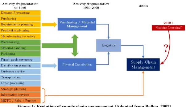
SCM deals with managing and assessing all components inside the supply chain (Figure 1). However, each of these components that comprise the supply chain network can be considered challenging and complex in isolation because of the prioritization of different, often competing objectives (e.g., low inventory levels, high on-time deliveries, low unit costs). Moreover, it is important to note that customers trigger SCM challenges. Certainly, demand forecasting is one of the main drivers of strategic decisions along supply chain tiers, which is why most organizations are investing and doing research on how to improve and predict future behavior (Waller, 2013). In this context, Barton and Court (2012) argue that predictive analytics is becoming a fundamental asset in many organizations to develop competitive advantages and focus on finding trends and patterns that help make optimal or at least better decisions.

(11)

Figure 1: Evolution of supply chain management (Adapted from Ballou, 2007)

Chopra and Sodhi (2004) identify various supply chain risks and drivers (Table 1). The mitigation strategy in which organizations fight or mitigate each threat will depend on the level of disruption encountered and how well-prepared organizations are (Chopra and Sodhi, 2004). Managers need to know the potential drivers that can cause supply chain risk to become uncontrollable or stable. Nevertheless, a common concept or “hidden” value is shared among all risks (Table 1). Being able to know how much is needed for selling or how many products should be produced can help identify: (1) how delays will affect Key Performance Indicators (KPIs), (2) how capacity will be limited, and (3) how much raw material is required in the warehouse. Therefore, researchers commonly agree that a major goal of SCM is to improve the forecasting accuracy, as a wrong prediction can lead to a variety of uncontrollable risks (Raghuantham, 2001).

(12)

Table 1: Supply chain risks and their drivers (Adapted from Chopra and Sodhi, 2004)

Risk Label Drivers of Risk

Disruptions

▪ Natural disaster

▪ Labor dispute

▪ Supplier bankruptcy

▪ Dependency on single source of supply Delays

▪ Quality errors

▪ Dependency on single source of supply

▪ Change in transportation modes

Systems ▪ System breakdown

▪ E-commerce

Forecasting

▪ Inaccurate forecast due to long lead times,

seasonality, product variety, short shelf life, small customer base

▪ “Bullwhip effect”, information distortion due to sales promotions, incentives, lack of supply chain visibility, and exaggeration of demand.

Intellectual Property ▪ Vertical integration of supply chain

▪ Global outsourcing and markets

Procurement ▪ _▪ Exchange rate changes

Long-term versus short-term contracts

Receivables ▪ _▪ # of customers

Financial strengths of customers Inventory

▪ Shelf life

▪ Product value

▪ Demand and supply uncertainty

Capacity ▪ _▪ Capacity flexibility

Production / storage costs

1.1. Demand Forecasting

Future demand typically is predicted or estimated by sales/marketing based on historical data and product life cycles (Brown et al., 2013). For most organizations, forecasting demand is of considerable importance, as they are aware of the consequences of using wrong values for purchasing materials, production planning, and workforce hiring (Carbonneau et al., 2008). Forecasting experts classify demand into four basic components (Brown et al., 2013):

1. Trend a steady increase or decrease over a certain time interval

2. Cycle patterns that repeat regularly over time 3. Seasonal high or low value during some time intervals

4. Random variations considered as “noise “inside the forecasting technique

(13)

Demand forecasting allows organizations to have an understanding of what they should expect in the next days/weeks/months. However, uncertainty caused mainly by random fluctuations and external factors (e.g., weather, politics, etc.) can distort the performance of how accurate forecasting calculations are. Hence, different forecasting techniques attempt to minimize the error value between the estimated value and reality.

Figure 2 shows the forecasting process managed by most organizations (Brown et al., 2013). The first step relies on collecting appropriate data. Today, this milestone has been improved by data mining techniques to ensure that the data will provide appropriate results. Then, a quantitative or qualitative forecast technique is selected to compute the estimations. Once these values are reviewed to ensure that they make sense to the core of the business, either an action is taken, or the method is revised if results are not convincing.

Figure 2: Process of forecasting (Adapted from Brown et al., 2013)

1.2. Data Mining

Forecasting is often based on historical data from organizations’ immediate customers. For this reason, results quality will be based on the data and method used. Data can be structured in different forms such as flat files, time series, images, and structured attributes (Fayyad and Uthurusamy, 2002). Weiss and Davison (2010) define data mining as an analytical process used to extract usable data from large datasets or unprocessed data for identifying possible patterns and trends. The process is structured in five sections: (1) selection, (2) pre-processing, (3) transformation, (4) modeling, and (5) interpretation. Items (1), (2), and (3) deal with identifying target values needed for the scope of the problem and transforming it into a standard format. Step (4) focuses on implementing algorithmic methods to fit and find hidden patterns in the processed data. Finally, Step (5) focuses on retrieving model results to give further feedback towards problem solutions and provide knowledge-driven decisions.

Today, data mining has become an effective tool in which organizations are willing to invest resources, as they can obtain competitive advantages (Menon et al., 2004). Han and Kamber (2011) establish the main usage of data mining as follows:

(14)

• Statistical analysis: there are several software packages (e.g., IBM SPSS, MaxStat, Minitab) that emphasize collecting and processing large data sets to find proper models.

• Data visualization: visualization models attempt to provide user-friendly, 2-D and multidimensional graphics for easier understanding and process of data.

• Parallel processing: structuring models to be executed using simultaneous processes can help to drastically reduce computational times and obtain faster results.

• Machine Learning (ML): using optimization algorithms and statistical models, ML manages to automate an analytical model’s training from historic data while minimizing the error or gap between an estimated value and reality.

Increasing market demand and customer requirements for better products are forcing companies to become more flexible and capable of forecasting large data sets to avoid losses in revenues or increased manufacturing costs (Wuest, 2014). Despite traditional methods providing a good approach to handle predictive analytics, data mining is proving to be effective for leading organizations to obtain even better results.

1.3. Forecasting Methods

Forecasting has always been an area of great importance for both academia and organizations. As previously discussed, acquiring knowledge about future behavior can lead to effective planning and allocation of resources, which in turn can lead to cost reductions and better KPIs. Nevertheless, finding an appropriate method to help make proper future decisions is a hard task. Hyndman and Athanasopoulos (2018) suggest that the power of prediction models is based on three factors: (1) how easily can data drivers be understood, (2) data set size, and (3) how well outputs obtained help aid future decision making.

Regardless of the forecast method used, it is essential that the model is capable of capturing both patterns and relations in the data without replicating random past events (Hyndman and Athanasopoulos, 2018). According to Armstrong (2001), forecasting methods will be always be influenced by the situation/environment on which they are tested or analyzed. The evaluation should consist of four steps: (1) testing assumptions, (2) testing data and methods, (3) replicating outputs, and (4) assessing outputs.

Brown et al. (2013) define three traditional forecasting methods: (1) time series, (2) causal methods, and (3) qualitative methods. Time series methods are based on how demand changes over time and look for trends in the data. Causal methods focus on how demand varies based on external or internal factors that might have affected it. Finally, qualitative methods, which are also known as the DelphiTechnique, use expert judgment to make decisions. In my thesis research, I focus on the time series methods described in the following subsections.

(15)

1.3.1. Moving Average (MA)

Nguyen et al. (2010) and Hansun et al. (2013) both discuss the quality of MA results. This technique is considered as the most common/basic approach for finding time series trends (Brown et al.¸ 2013). The technique consists of calculating a set of averages, where each average corresponds to a trend value inside some time period or interval. Indeed, each new average overlaps a set of new values based on the period. The term moving average comes from the fact that each average is computed by replacing the oldest observation by the next data point. This method is a type of mathematical convolution (Hyndman, 2011). The moving average of order 𝑚, where 𝑚 is odd, can be written as:

𝑍̂𝑡 = 1 𝑚 ∑ 𝑦𝑡+𝑗 𝑘 𝑗=−𝑘 ; ∀ 𝑡 = 𝑘 + 1, … , 𝑛 − 𝑘

o 𝑚 = 2𝑘 + 1 moving average of order 𝑚. Also, known as ′𝑚(𝑜𝑑𝑑) − 𝑴𝑨′

o 𝑛 total number of data points used

On the other hand, for the case where 𝑚 is even, the calculation is as follows: 𝑍̂_𝑡 = 1

𝑚∑ 𝑦𝑡−𝑗

𝑘

𝑗=0

; ∀ 𝑡 = 𝑘 + 1, … , 𝑛

o 𝑚 = 𝑘 + 1 moving average of order 𝑚. Also, known as ′𝑚(𝑒𝑣𝑒𝑛) − 𝑴𝑨′

o 𝑛 total number of data points used

For the second case (𝑚 –even), it is important to align the averages obtained in the middle of the data values being averaged. Otherwise, it will cause the analysis of trend lines to be more difficult. This procedure is called ‘centered moving average’ or 2 × 𝑚(𝑒𝑣𝑒𝑛) MA. Further, a moving average can itself be smoothed by another moving average, also known as a double moving average (Hyndman, 2011). Finally, moving averages can treat each past period equally or unequally (weighted moving average).

1.3.2. Exponential Smoothing (ES)

Exponential smoothing has also provided companies with successful and promising results since 1950 (Brown et al. 2013). Exponential smoothing computes weighted averages of past observations, where the weights decay exponentially in time. This approach gives more weight or importance to the most recent observations (Hyndman and Athanasopoulos, 2018). Simple exponential smoothing is considered as the most basic approach, particularly when the data has no clear trend or seasonal pattern. Observations further from the current time value ‘T’ have smaller weights assigned to them. Hyndman and Athanasopoulos (2018) give the following equation for calculating ES forecasting values:

𝑦̂𝑇+1 | 𝑇= 𝛼𝑦∙𝑇+ 𝛼(1 − 𝛼)𝑦∙𝑇−1+ 𝛼(1 − 𝛼)𝑦∙𝑇−22 + ⋯ ; ∀ 0 ≤ 𝛼 ≤ 1

The term 𝛼 is a smoothing parameter that controls the rate of exponential decay for each past variable over the range analyzed. The future value 𝑦̂_𝑇+1 is a weighted average

(16)

based on all previous observations 𝑦₁, 𝑦₂, ⋯ , 𝑦_𝑇 controlled by the smoothing parameter 𝛼. As 𝛼 gets closer to zero (one), larger weights are assigned to older (newer) observations. In the case when 𝛼 = 1, this is the same as naïve forecasting, as the most recent observation is the only value which provides information about the future.

Extending the concept of Exponential Smoothing, Siregar et al. (2017) describe the importance of using Double Exponential Smoothing on splitting the trend component into two variables, commonly named as 𝛼 and 𝛽, to try smooth the trend in the time series data. The two equations of DES are:

𝑠_𝑡= 𝛼 ∙ 𝑦_𝑡+ (1 − 𝛼) ∙ (𝑠_𝑡+1+ 𝑏_𝑡−1) ; ∀ 0 ≤ 𝛼 ≤ 1 𝑏_𝑡 = 𝛽(𝑠_𝑡− 𝑠_𝑡−1) + (1 − 𝛽) ∙ 𝑏_𝑡−1 ; ∀ 0 ≤ 𝛽 ≤ 1

𝑠_𝑡+𝑚 = 𝑠_𝑡+ 𝑚 ∙ 𝑏_𝑡; ∀ 𝑚 > 0

In these equations, 𝑠_𝑡 is the smoothed value at time t, 𝑏_𝑡 is the approximation of the trend at time t, and m is the period for the forecast.

Finally, Triple Exponential Smoothing can be considered when dealing with seasonality in the time series data. In addition to α and β, a new variable γ is introduced to model/control the influence of seasonality. Siregar et al. (2017) argue that Triple Exponential Smoothing is the most advanced variation of Exponential Smoothing, as it attempts to develop both double and simple exponential smoothing together, adding the seasonal period into it. Hence, properly defining the period is crucial for the forecast to work properly. For instance, if the series was monthly data and the seasonal period repeats every six months, then the period should be set as six.

Triple Exponential Smoothing is defined by: 𝑠_𝑡= 𝛼 ∙ 𝑥𝑡 𝑐𝑡− 𝐿 + (1 − 𝛼) ∙ (𝑠_𝑡−1+ 𝑏_𝑡+1) ; ∀ 0 ≤ 𝛼 ≤ 1 𝑏_𝑡 = 𝛽(𝑠_𝑡− 𝑠_𝑡−1) + (1 − 𝛽) ∙ 𝑏𝑡−1 ; ∀ 0 ≤ 𝛽 ≤ 1 𝑐_𝑡 = 𝛾 𝑥𝑡 𝑠_𝑡+ (1 − 𝛾) ∙ 𝑐𝑡−𝐿 ; ∀ 0 ≤ 𝛾 ≤ 1

In these equations, 𝑥_𝑡 are the sequence of observations with a cycle of season change L; 𝑠_𝑡is the sequence of seasonal corrections; 𝑏_𝑡 is the sequence of best estimates of the linear trend; and 𝑐_𝑡 is the sequence of best estimates of the seasonal factors. Based on Hyndman and Athanasopoulos (2018), 𝑐_𝑡 is the expected proportion of the trend forecast at any time 𝑡 𝑚𝑜𝑑 𝐿 based on the number of periods defined.

It is important to state that when trying to model trend or seasonality, it can be modeled as either additive (where the seasonality, trend, and noise are added) or multiplicative (where the seasonality, trend, and noise are multiplied). For instance, in the case of Triple Exponential Smoothing, it will be defined as follows:

• Additive: 𝑆_𝑡+, = (𝑠_𝑡) + (𝑚 ∙ 𝑏_𝑡) + (𝑐_{𝑡−𝐿+𝑚}) 𝑚𝑜𝑑 𝐿; ∀ 𝑚 > 0 • Multiplicative: 𝑆_𝑡+, = (𝑠_𝑡) ∙ (𝑚 ∙ 𝑏_𝑡) ∙ (𝑐𝑡−𝐿+𝑚) 𝑚𝑜𝑑 𝐿 ; ∀ 𝑚 > 0

(17)

1.3.3. Auto-Regressive Integrated Moving Average (ARIMA)

Both ES and ARIMA models are two of the most frequently used methods in time series forecasting (Brown et al., 2013). While ES relies on weighting past values based on the description of the trend and seasonality in the data, ARIMA aims to find the autocorrelations inside the data (Hyndman and Athanasopoulos, 2018). This technique combines multi-variate regression analysis (autoregressive models) with time series models (MA) to find effective results (Brown et al., 2013).

To better understand ARIMA, it is important to distinguish how the

autoregressive section links with the MA part. In an autoregressive model, predicted values are calculated using a linear combination of past values. Hyndman and

Athanasopoulos. (2018) define an autoregressive model of order 𝑝 as ‘𝐴𝑅(𝑝)’ model: 𝑦_𝑡 = 𝑐 + (𝜙₁∙ 𝑦_𝑡−1) + (𝜙2∙ 𝑦𝑡−2) + ⋯ + (𝜙𝑝∙ 𝑦𝑡−𝑝) + 𝜀𝑡

o 𝜀_𝑡 is defined as white noise or randomness. This will affect the scale of the series but not the pattern.

o 𝜙_𝑝 depends on the order p selected

o 𝑐 = (1 − ∑𝑝_𝑖=1𝜙_𝑖) ∙ 𝜇_{𝑝𝑟𝑜𝑐𝑒𝑠𝑠}

The value of 𝑐 refers to the average change between consecutive observations. If 𝑐 > 0, then the values are increasing over time; otherwise, the trend is moving downwards. Hence, depending on model order, 𝜇𝑝𝑟𝑜𝑐𝑒𝑠𝑠 will be the mean of consecutive observations

considered.

Hyndman and Athanasopoulos (2018) recommend restricting autoregressive models to stationary data as it is important to understand that changing parameters 𝜙1, ⋯ , 𝜙𝑝 will lead to different time-series patterns. The authors recommend the following

constraints for the best outcomes:

o 𝐴𝑅(1) 𝑚𝑜𝑑𝑒𝑙 − 1 ≤ 𝜙1 ≤ 1

o 𝐴𝑅(2) 𝑚𝑜𝑑𝑒𝑙 − 1 ≤ 𝜙1 ≤ 1 ; 𝜙1+ 𝜙2 < 1 ; 𝜙2− 𝜙1 < 1

o For 𝑝 ≥ 3, the restrictions are more complicated, which can lead to higher computational times.

The second parameter of an ARIMA(p, d, q) model refers to the degree of first differencing. Differencing refers to keeping track of the differences between consecutive observations. The main objective of this parameter is to stabilize the mean of a time series by reducing or eliminating the influence of trend and seasonality. Regarding the MA model, instead of using past values, the model uses past forecast errors. The MA model of order 𝑞 is referred as ‘𝑀𝐴(𝑞)’

(18)

As seen in moving averages, as 𝜃 > 1, the weights increase leading to a higher level of influence on the current error. Like autoregressive models, Hyndman and Athanasopoulos (2018) recommend the following constraints:

o 𝑀𝐴(1) 𝑚𝑜𝑑𝑒𝑙 − 1 ≤ 𝜃1 ≤ 1

o 𝑀𝐴(2) 𝑚𝑜𝑑𝑒𝑙 − 1 ≤ 𝜃1 ≤ 1 ; 𝜃1 + 𝜃2 < 1 ; 𝜃2− 𝜃1 < 1

o For 𝑞 ≥ 3, the restrictions are more complicated, which can lead to higher computational times.

Summarizing the points above, an ARIMA model will be determined by order of the autoregressive part (p), degree of first differencing involved (d), and order of the moving average part (q). However, how should each parameter be chosen? The package Akaike’s

Information Criterion (AIC) can be used for determining the values of an ARIMA model as follows (Hyndman and Athanasopoulos, 2018):

𝐴𝐼𝐶 = −2 log(𝐿) + 2(𝑝 + 𝑞 + 𝑘 + 1)

In this equation, 𝐿 is the likelihood of the data (the higher the value, the better fit), 𝑘 = 1 if 𝑐 ≠ 0 and 𝑘 = 0 if 𝑐 = 0. Although the AIC approach gives a good way to find the value of 𝑝 and 𝑞, it is not appropriate for determining what value of 𝑑 should be used. This occurs because different levels of 𝑑 will change the value of likelihood (𝐿), so AIC values for different value of 𝑝 and 𝑞 cannot be compared.

1.4. Machine Learning

Machine Learning (ML) has recently gained significant acceptance among both academic researchers and practitioners (Makridakis et al., 2018). ML approaches, like statistical methods, aim to minimize a loss function (i.e., the difference between predicted vs. real value) which is typically calculated as some function of the sum of squared errors. However, while statistical methods usually use linear processes, ML methods often rely on nonlinear algorithms (Makridakis et al., 2018).

When building ML models for use as forecasting tools, some portion of the available data (e.g., 80%) is used to teach or train the model (“training dataset”), while the remaining data (e.g., 100%-80% = 20%) is used to test the model’s expected performance (“testing dataset”). It is important to focus on generalization, overfitting, and underfitting when using ML techniques (Müller, 2016). Generalization is possible when the ML model is capable of accurately predicting results for unseen data, as the model can generalize future results from the training set. Next, overfitting occurs when the results obtained are to close the ones used in the training set only, but not for unseen data, often because too much of the available data was used for training (e.g., >95%). Underfitting occurs when the model’s training data is insufficient and/or there are not enough factors in the training set—this can lead to wrong predictions, both in the training and testing datasets.

As shown in Figure 3, finding trustworthy parameters for ML models can prove to be a hard task. As we increase (decrease) the model’s complexity, the more likely overfitting (underfitting) occurs. Indeed, the aim is to achieve the ‘sweet spot’ to get the

(19)

smallest value for the loss function. The data used for both training and testing must be obtained from a pre-processing process to avoid distortion factors and model what is important to analyze.

1.4.1. K-Nearest Neighbor (K-NN) Regression

The K-NN algorithm compares the training set with new unseen data and makes a prediction based on finding the closest distance (e.g., Euclidean distance) between training data points, also known as their “nearest neighbor,” to the point at which we want to make the prediction (Müller and Guido, 2016). Figure 4 shows three new points (green stars) and where, based on the distance to the closet training points, their target values are estimated to be (blue stars).

Figure 3: Trade-off Model Training and Test accuracy (Adapted from Müller and Guido, 2016)

Figure 4: Examples of predictions using different values of neighbors (Adapted from Müller and Guido, 2016)

As mentioned previously, K-NN is based on learning by analogy. Indeed, any new instance is associated with its k-closest instances inside the training set of n-dimensions as an attempt to classify it with similar behavior as their neighbors (Martinez et al., 2019).

(20)

All weights (closet distances) can be averaged to predict what target value should be assigned to the unseen data:

𝑧_𝑇 = ∑𝑡 𝑖 𝑘 𝑘 𝑖=1 𝑤ℎ𝑒𝑟𝑒 𝑡𝑖 _{= 𝑑𝑖𝑠𝑡𝑎𝑛𝑐𝑒 𝑏𝑒𝑡𝑤𝑒𝑒𝑛 𝑒𝑎𝑐ℎ 𝑖}𝑡ℎ_{𝑡𝑟𝑎𝑖𝑛𝑖𝑛𝑔 𝑎𝑛𝑑 𝑡ℎ𝑒 𝑛𝑒𝑤 𝑖𝑛𝑠𝑡𝑎𝑛𝑐𝑒 𝑝𝑜𝑖𝑛𝑡}

Figure 5 shows the influence of using different numbers of neighbors. While a low number of neighbors can make the model behave as an overfit model, a high number of neighbors can result in underfitting. For instance, the training score shown measures the accuracy of the model to predict the true value. When the model is overfit, the training score is 100%, causing the test score to be low (35%) and vice versa. Hence, sensitivity analysis is crucial for finding the precise parameter for obtaining the best results (‘sweet spot’).

Figure 5: Examples of predictions using different values of neighbors (Adapted from Müller and Guido, 2016)

1.4.2. Ensembles of Decision Trees (Random Forests)

Decision trees are well-known models for classification and regression approaches. The learning process for both regression and classification involve a series of if/else questions to make a decision. However, the main problem of using decision trees is that they tend to overfit the data (Müller and Guido, 2016). Hence, ensembles (collections) of decision trees were created to attempt to solve this problem. The two most common methods are random forests and gradient-boosted decision trees.

Random forests are a combination of tree predictors where each tree generated will be dependent on the random vector values sampled. The idea of building as many trees as possible is to decrease the overfitting factor using the average of all predictions (Breiman, 2001). Figure 6 represents graphically how the reduction of overfitting is achieved by the average of all trees. Similarly, gradient-boosted decision trees also build decision trees, but on each new tree, it attempts to fix the errors resulting from the previous one. Hence, no

(21)

randomization is used as each new tree will prune the previous one to improve it (Müller and Guido, 2016).

Figure 6: Random forest structure (Adapted from Breiman, 2001)

1.4.3. Neural Networks models (NN) Models (Deep Learning)

Neural networks arose from an attempt to replicate the behavior of the human brain. These models allow merging different non-linear relationships along with the data set (response variables) and its predictors (Hyndman and Athanasopoulos, 2018). Indeed, neural networks are deep learning methods (also known as Multilayer perceptrons (MLPs)) which are viewed as multiple stages of linear models (Müller and Guido, 2016). The neural network is structured by the inputs (also known as predictors), n hidden layers, and the target forecasts (output) (Figure 7).

Figure 7: Single hidden layer Neural Network (Adapted from Müller and Guido, 2016)

If 𝑛 = 0 (i.e., no hidden layer), this is model is equivalent to a classical linear regressor as follows: 𝑦̂ = (𝑤[0] ∙ 𝑥[0]) + ⋯ + (𝑤[𝑝] ∙ 𝑥[𝑝]) + 𝑏. For all 𝑤[0], ⋯ , 𝑤[𝑝] it represents the learned coefficient (weight) of each predictor (input) as 𝑥[0], ⋯ , 𝑥[𝑝]. The target forecast value 𝑦̂ is obtained by a linear combination of the input. Before obtaining this final value, each intermediate value between the defined layers is calculated

(22)

by receiving the input from the previous layer. Therefore, the forecast value is defined as a weighted sum of each of the previous layers (Müller and Guido, 2016). The weights assigned to each connecting line are assigned by using a ‘learning algorithm’ (e.g., sigmoid function, rectifying function, or tangent hyperbolicus function) that minimizes the loss function defined (e.g., mean squared error or root mean square error).

When initializing a neural network, the weights take random values and then are updated using the observed data. In order to increase the accuracy of the model and minimize the effect of randomness, the network is trained several times using different starting points. It is important to define the number of nodes inside hidden layers a priori. However, this parameter should be defined based on seasonality, stationarity, and trend features of the data (Hyndman and Athanasopoulos, 2018) Figure 8 represents an example of a 30-year forecast of solar magnetic fields affecting communication networks that used six hidden layers.

Figure 8: 30 years forecasting using 6 hidden layers (Adapted from Hyndman and Athanasopoulos, 2018)

(23)

CHAPTER TWO: DATASETS AND METHODOLOGY

In this chapter, two datasets are analyzed using traditional and machine learning methods. The first dataset is divided into four subgroups where each subgroup is characterized by high levels of variability and a different number of observations. The second dataset is defined by lower variability and many records (>15K), where the most demanded product at different warehouse locations is analyzed. Lastly, the first dataset pertains to the forecasting of production plans, while the second dataset predicts future demand behavior.

2.1. Dataset 1: Office Supplies

The first dataset in this thesis is from a real-world production environment, collected over the five-year period between 2015 and 2019. In total, 1510 SKUs are detailed which belong to 285 product families. The data is from a report for each SKU’s movement and calculates the difference between actual consumption and errors when confirming quantities. These two movement types are grouped by ‘Mvt 101’ (quantity consumed) and ‘Mvt 102’ (quantity don’t exist). Hence for any day, the real quantity in the system should be the grand sum of (𝑀𝑣𝑡 101 − 𝑀𝑣𝑡102) for each SKU.

When looking at the quantities per family product, it was found that 44% was mainly driven by two groups (families): Ballpoint pen XYZ and Marker ABC. For this reason, the thesis research will focus on these two families’ products. Figure 9 displays the relationship between the research focus in products and all SKUs involved:

Figure 9: Distribution of Products

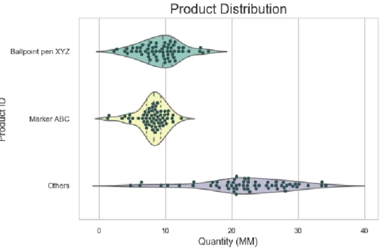
Moreover, Figure 10 shows a violin plot of the quantity demanded for the two product families of interest and all products. This plot helps to merge the results obtained from the box plot with its density plot. It was found that on average Ballpoint XYZ has a monthly production of 10 million (MM), while Marker ABC sees monthly production of

(24)

8.7 MM units. The remaining families (283 groups, ~ 1067 SKUs) are widely spread with an average production of 20MM per month.

Figure 10: Quantity Distribution of production quantity based on family’s product

2.1.1. Analysis for SKU Marker ABC

Products within family Marker ABC are identified based mainly on their final customer destination. A Pareto analysis (Figure 11) was used to determine which SKUs should be analyzed in detail. For research purposes, only Marker ABC will be considered, as it represents 62% of the total production of the product family. To avoid any outliers that could mislead our forecasting methods under study, all values outside of ±3σ of the mean (i.e., yellow shaded area in Figure 12) are dropped from the dataset.

(25)

Figure 11: Pareto Principle for Marker ABC group

Figure 12: Time Series Production per week for Marker ABC

As an initial data visualization step, a histogram was plotted for the Marker ABC data (Figure 13) and the fit of various probability distributions to the data was determined by evaluating squared error (Table 2). Based on the square error results, it follows that the gamma distribution provides the most suitable fit for the Marker ABC weekly production data.

(26)

Figure 13: Probability density for daily production for Marker ABC Table 2: Distribution Summary for Marker ABC

Distribution Square Error

Marker ABC Beta 0.011213 Erlang 0.024651 Exponential 0.024651 Gamma 0.007583 Lognormal 0.046134 Normal 0.017115 Triangular 0.012056 Uniform 0.046885 Weibull 0.0089

2.1.2. Traditional Forecasting Models for Marker ABC 2.1.2.1. Moving Average (MA)

Window sizes between two and 10 were tested to analyze the performance of Moving Average models. Figure 14 displays how each of the models attempts to fit the data based on its parameters for the weekly production. It shows that as we increase the order, we reduce the amplitude towards the mean value of the average production. Moreover, for MA = 2, the model seems to overfit (model predictions are very close to true values) the predicted values, which leads to doubt about the performance of the models even though it has the smallest error.

(27)

Figure 14: Output for different levels of Moving Average (order 2, 5, 7, 10)

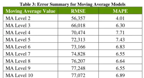
Table 3 and Figure 15 describes the MAPE and RMSE errors found for each of the different parameters used under MA. As mentioned early, MA = 2 gives the best results for predicting weekly production, which implies that the best prediction is expected to be of ±2 production days. Moreover, to forecast short term values, it is likely that values will appear stationary.

Table 3: Error Summary for Moving Average Models

Moving Average Value RMSE MAPE

MA Level 2 56,357 4.01 MA Level 3 66,018 6.30 MA Level 4 70,474 7.71 MA Level 5 72,313 7.43 MA Level 6 73,166 6.83 MA Level 7 74,828 6.55 MA Level 8 76,207 6.64 MA Level 9 77,248 6.55 MA Level 10 77,072 6.89

(28)

Figure 15: MAPE and RMSE Error vs MA Order level

2.1.2.2. Simple Exponential Smoothing (SES)

As discussed previously, Simple Exponential Smoothing uses the α parameter to fit the data. Figure 16 compares the RMSE of different alpha values when being tested on the weekly production values for Marker ABC. To measure how the forecast works, the last four weeks of available data will be used to test the accuracy of SES. From the results, as alpha values increase, so does RMSE. This implies that small α values should be used. Indeed, the best parameter was defined to be α = 0.05 with an RMSE error of ±83K referring to ±3.5 days of production.

Figure 16: RMSE behavior using different alpha levels

Table 4 summarizes the error found for both the training set and testing set, which are shown to be comparable in scale, thereby confirming our expectation of a properly fit SES model.

Table 4: Error Summary for Simple Exponential Smoothing - Marker ABC

Training Set Forecast (4 weeks)

Parameters RMSE MAPE RMSE MAPE

(29)

Figure 17 describes how the best 𝛼 = 0.05SES models the data provided. However, when using the model to forecast future behavior, a constant / stationary value is predicted, as no new recent actual data is available for calculations. This, in turn, can lead to wrong interpretations by decision makers.

Figure 17: Simple Exponential Smoothing plot with different α values

2.1.2.3. Double Exponential Smoothing (DES)

Regarding DES, the trend parameter ß used to smooth slope tries to improve the overall model fit. Table 5 summarizes the accuracy results obtained using the best parameters found in our analyses: 𝛼 =0.1 and 𝛽 =0.15. Figure 18 shows how model error changes when using different combinations of alpha and beta.

Figure 18: RMSE behavior for different combination of alpha and beta Table 5: Error Summary for Double Exponential Smoothing - Marker ABC

(30)

Alpha = 0.1; Beta = 0.15 85,005 0.57 77,454 0.49

Figure 19 shows how the DES model works on the data provided. In contrast to SES, the DES forecast suggests a linear upward trend in its future forecast. As for the training set, the fit DES model seems to describe more accurately the behavior of the data compared to the SES, as the linear trend is evident in Figure 19.

Figure 19: Double Exponential Smoothing plot using best α and ß values

2.1.2.4. Triple Exponential Smoothing (TES)

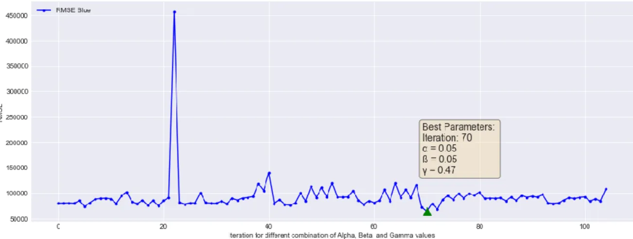
For the TES, both multiplicative and additive methods were tested to find the best combination of parameters that yield the smallest RMSE. Figure 20 describes the results obtained for the best combination: 𝛼 = 0.05, 𝛽 = 0.05, and 𝛾 = 0.47. Indeed, TES provides more realistic modeling of the data compared to the previous cases analyzed, as both linear and seasonal trends are considered. Table 6 shows the best fit results found in the analysis.

(31)

Figure 20: RMSE behavior for different combinations of alpha, beta, and gamma Table 6: Error Summary for Triple Exponential Smoothing - Marker ABC

Alpha = 0.05

Beta = 0.05; Method: Add γ = 0.47; Method: Mult

77,893 0.57 64,176 0.49

Figure 21 describes how the TES models the data under study. Despite the initial outliers seen in the first year, overall TES does fit the data more accurately than the other two ES methods studied. In contrast to SES and DES, the RMSE error is ±1 day better than the other two ES models evaluated.

(32)

2.1.2.5. ARIMA

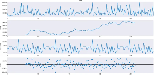
ARIMA models are typically characterized by being more flexible when modeling time series data. Figure 22 provides the decomposition of the time series data into trend, seasonality, and residual (noise). From these results, there is a positive trend with a repetitive seasonality every 75 weeks. Also, the residual (noise) seems to be constant in time with no discernible behavior or pattern.

Figure 22: Decomposition of Trend and Seasonal feature for Marker ABC

When building an ARIMA model, it is important to obtain appropriate values for parameters p, d, and q. An iterative grid search is used to evaluate each possible combination of parameters in the model. After evaluating all possible combinations, we will evaluate each combination using the Akaike Information Criterion (AIC), as AIC measures the performance of how well the parameter chosen models the training dataset. As a high value of AIC means that more features are being used to model the data than necessary, the target is to choose the parameter combination which provides the smallest AIC score.

From the results obtained, the ARIMA parameters (1, 0, 1) (0, 1, 1, 12) yield a best possible AIC score of 5454.04. With these parameters, we can further investigate the model and see if any unusual behavior is present. When analyzing how the model is forecasting the data, the main goal is to see if the residuals are uncorrelated and normally distributed ~𝑁(0,1). Based on Figure 23, the histogram gives a good indication that our residuals are ~𝑁(0,1), despite the Kernel Density Estimation (KDE) having a slightly higher standard deviation. Hence, because of this small variation, the blue dots on the Normal Q-Q plot do not follow a linear trend perfectly. Finally, the correlogram which compares the lag between datapoints suggests that the correlations are very low and do not follow any pattern.

(33)

Figure 23: Diagnostics for ARIMA model

Table 7 summarizes the results obtained using the best fit ARIMA model, while Figure 24 shows how the ARIMA model fits the Marker ABC dataset.

Table 7: Error summary for ARIMA model

Training Set Forecast (15 days)

Method RMSE MAPE RMSE MAPE

ARIMA (1, 0, 1) (0, 1, 1, 12) 82,086 1.87 84,603 10.23

Based on the experimental results, the RMSE errors are not significantly better compared to the previous forecast methods used. The reason for this could be due to the variation found on the residuals and the low relationship between lags greater than one. Another reason could be because the weekly values have a standard deviation of 132K, which makes it difficult to produce an accurate forecast value. Hence, most traditional forecast methods will attempt to trend towards the mean value.

(34)

Figure 24: ARIMA (1, 0, 1) (0, 1, 1, 12) model for fitting Marker ABC data set

2.1.3. Machine Learning Forecasting Models for SKU Marker ABC

When using ML methods, one of the main challenges to determine is the percentage of data required to train and test the model. If data is not big enough this may lead to good training, however, not necessarily too good testing results of the data. Hence, this will be an area of focus in the following analysis and discussion.

2.1.3.1. K-Nearest Neighbors (KNN)

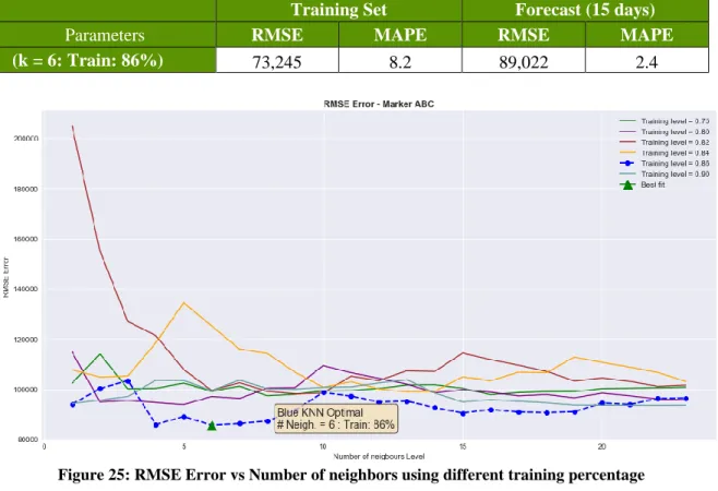
For the KNN algorithm, the main parameter of interest is how many neighbors will be used to fit the data. Based on the sensitivity analysis shown in Figure 25, the best value is obtained by using a training percentage of 86% and number of neighbors equal to six.

(35)

Table 8: Error summary for KNN 86% Training data and neighbors=6

Parameters RMSE MAPE RMSE MAPE

(k = 6: Train: 86%) 73,245 8.2 89,022 2.4

Figure 25: RMSE Error vs Number of neighbors using different training percentage

Even though the RMSE error for the training set is 73,245, when using the model to obtain the forecast, the KNN model predicted values as a horizontal fixed mean value (i.e., the red line in Figure 26). Possible reasons for this might be due to not enough data being available to train the model. Figure 26 shows the comparison between the modeling of the training data against the forecasted values produced by the KNN method.

Figure 26: KNN – Modeling of Training data vs Forecast data

2.1.3.2. Decision Tree

The Decision Tree (DT) ML method builds regression models in the form of a tree structure. Figuring out the proper depth that the tree should be is important to obtain the best results. Moreover, what predictors will be inside the DT will also affect how forecast

(36)

values are calculated. Since we are using time series data, our target values are the demand levels and the predictors are the individual date values. However, for the date values, it is necessary to break down the date values to appropriately know how target values are affected by each feature. Table 9 shows an example of how data is used inside the DT algorithm via feature engineering:

Table 9: Breaking down of time series dates into features

Figure 27 provides the findings when testing the DT algorithm under different training sets and changing the depth of the tree. It was found that a training set of 65% and a depth of two were the best parameters for predicting the desired results, based on the smallest RMSE. Finally, Table 10 and Figure 28 provide the error summary of the model using the best parameters found and a visual representation of the DT fit, respectively.

Figure 27: Decision Tree – Modeling of Training data vs depth of tree

True Demand Month end? Month Start? Quarer end? Quarter Start? Year end? Year

start? Year Month Week Day

Number days elapsed in the year Numeric value 87293 0 0 0 0 0 0 2015 1 3 12 12 1421020800 33120 0 0 0 0 0 0 2015 2 7 9 40 1423440000 9459 0 0 0 0 0 0 2015 2 8 16 47 1424044800 129226 0 1 0 0 0 0 2016 2 5 1 32 1454284800 […] […] […] […] […] […] […] […] […] […] […] […] […]

(37)

Table 10: Error summary for Decision Tree 65% Training data and depth =2

(DT Depth = 2: Train: 65%) 66,903 7.6 98,795 1.2

Figure 28: Decision Tree – Modeling of Training data vs Forecast data

2.1.3.3. Ensembles of Decision Trees (Random Forests)

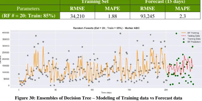
Ensembles or groups of decision trees can indeed produce better forecasting results than DTs alone as the ensemble uses several decision trees to make its decisions. Hence, obtaining what percentage of training data and the number of trees to create is critical to model time series data using this approach which is commonly known as a Random Forest (RF). Figure 29 provides the findings after testing the RF algorithm under different training sets and changing the number of trees. Results suggest that a training set of 85% and generating 20 trees provides the best (smallest) RMSE. Finally, Table 11 and Figure 30 depict the results obtained under these parameters in terms of error and data visualization.

(38)

Table 11: Error summary for Ensembles Decision Tree 85% Training data and number of trees = 20

(RF # = 20: Train: 85%) 34,210 1.88 93,245 2.3

Figure 30: Ensembles of Decision Tree – Modeling of Training data vs Forecast data

2.1.3.4. Recurrent Neural Network

Time series forecasting using Recurrent Neural Networks (RNN) is a useful tool for analyzing sequential data. For this research, we are using the Long Short-Term Memory (LSTM) model to translate our data into a forecast model. According to Karim et al. (2017), LSTM models enhance the performance of the whole network allowing the use of minimal preprocessing or dataset training. Under this premise, it is fundamental to determine the best training set, the number of epochs, and the number of hidden layers to use in the network. Figure 31 summarizes how the RMSE changes under different combinations of training levels with hidden layers. For each training level an array of 15, 25, 30, 40, 50 and 55 hidden layers were tested. Hence, the vertical drop shown at each training level. The tradeoff between the training set and the RMSE error of the testing set converges at a training level of 90%. It is important to see that as the RMSE error decreases for the training set (green dotted line), the testing sets starts to be less accurate, suggesting that we may be moving away from the ‘sweet spot’ towards overfitting.

(39)

Using these initial results, the next step is to find the number of epochs that fits our data best to avoid unnecessary model complexity. Based on Figure 32, the best value is obtained at 12 epochs; this is where the model MSE is a minimum.

Figure 32: LSTM loss / error versus number of epochs used

Table 12 and Figure 33 summarize the results obtained for the RNN model. Indeed, the RMSE error obtained is similar to the values found with DT, RF, and KNN. The errors suggest that the model will have an offset ±4 days of production, as the original data source reveals daily production of 20K-25K per day, on average. Possible reasons for this could be due to the high variability of weekly production between each time step. For instance, a week of 50K units of production is followed by a 300K week. This large deviation can indeed prove difficult to model and fit with any candidate approach.

Table 12: Error Summary for RNN – LSTM model for Marker ABC

Training Set Testing Set

Method RMSE MAPE RMSE MAPE

RNN – LSTM Layers: 15 % Train: 90% Epochs: 12

72,742 7.8 77,960 1.02

(40)

2.1.4. Analysis for SKU Ballpoint pen XYZ

After analyzing the Ballpoint XYZ dataset, 88 SKUs were found. Ballpoint XYZ is comprised of a range of products that are either a mix or single-color ballpoint pen from a set of 12 colors. Hence, instead of focusing on 88 SKUs, we look at one level upstream in the product’s bills of materials, it is possible to narrow the research to ballpoint pen units. A Pareto analysis (Figure 34) shows which colors actually drive the production plans for this product family. Clearly, 86% of 2015-2019 production corresponds to blue, black, and red pen colors. Looking at each individual color, blue (50%) represents production of 1.1 MM per week, with black (21%) and red (15%) constituting 0.46 MM and 0.42MM per week, respectively.

Figure 34: Pareto Principle for Ballpoint Pen XYZ colors

To avoid outliers that could mislead the forecasting approaches under study, as done with the previous dataset, only values inside of ±3σ of the mean (yellow shaded area in Figure 35) will be used in the analysis.

(41)

Figure 35: Time Series Production per day for Ballpoint Pen XYZ color blue, red, and black

In order to analyze weekly behavior by color, each color was fit to a standard statistical distribution. Based on the square error, we found that blue pen production follows a Beta distribution, while black and red production follows an Exponential distribution. Table 13 gives the errors found per distribution, while Figure 36 shows a graphical visualization for each best fit. We now turn our attention to assessing the fit of traditional and machine learning methods for forecasting this time series data.

Table 13: Distribution Summary per color

Distribution / Color

Square Error

Blue Black Red

Beta 0.001712 0.005452 0.008594 Erlang 0.00637 0.003501 0.006845 Exponential 0.00637 0.003501 0.006845 Gamma 0.005471 0.0487 0.007043 Lognormal 0.028516 0.032946 0.032105 Normal 0.017631 0.036141 0.049301 Triangular 0.006306 0.025838 0.03393 Uniform 0.02884 0.065276 0.074598 Weibull 0.005032 0.003858 0.006855

(42)

Figure 36: Probability density for weekly production for Ballpoint Pen XYZ color blue, red, and black

2.1.5. Traditional Forecasting Models for SKU Ballpoint Pen XYZ 2.1.5.1. Moving Average

Following the same methodology as Marker ABC, Table 14 and Figure 37 portray the results obtained after fitting the data using moving average. The smallest error was obtained by using an MA level of two. According to the production daily capacity, the RMSE error found represents ±12 hours of production. Indeed, these results suggest that the model values obtained could be quite useful for forecasting production.

Table 14: Error Summary for Moving Average Models

Moving Average Value

RMSE MAPE Average

Blue Black Red Blue Black Red RMSE MAPE

MA = 2 71,664 48,446 42,889 0.27 0.35 0.27 54,333 0.30 MA = 3 87,126 59,756 52,963 0.34 0.44 0.34 66,615 0.37 MA = 4 93,319 66,485 58,755 0.36 0.50 0.37 72,853 0.41 MA = 5 99,283 69,205 59,531 0.39 0.52 0.38 76,007 0.43 MA = 6 102,826 70,770 60,768 0.40 0.54 0.38 78,121 0.44 MA = 7 103,243 71,555 60,991 0.41 0.55 0.39 78,596 0.45 MA = 8 104,412 71,825 62,795 0.41 0.56 0.40 79,677 0.46 MA = 9 104,820 72,092 63,522 0.42 0.56 0.40 80,145 0.46 MA = 10 106,615 72,420 63,873 0.42 0.57 0.41 80,969 0.46

(43)

Figure 37:MAPE and RMSE Error vs MA Order level

Figure 38 describes how each MA level in Table 14 attempts to fit in the data. Because MA is sensitive to rapid demand changes, this model is hard to use when the goal is to forecast production beyond one period, especially if seasonal behavior is present. As the level of MA increases, the model starts to converge to the mean value and the difference between true demand and predicted demand starts to increase.

Figure 38: Modeling of MA for Ballpoint Pen XYZ

2.1.5.2. Simple Exponential Smoothing

Figure 39 shows how RMSE changes when using different alpha values in SES. For blue and red pens, the best alpha values are relatively small, while black pens see a