Modeling and measuring insurance risks for a hierarchical copula model considering IFRS 17 framework

(1)

Modeling and measuring insurance risks for a hierarchical copula model

considering IFRS 17 framework

Carlos Andr´

es Araiza Iturria

A Thesis

in

The Department

of

Mathematics and Statistics

Presented in Partial Fulfillment of the Requirements

for the Degree of Master of Science (Mathematics) at

Concordia University

Montreal, Quebec, Canada

June 2019

(2)

CONCORDIA UNIVERSITY

School of Graduate Studies

This is to certify that the thesis prepared

By: Carlos Andr´es Araiza Iturria

Entitled: Modeling and measuring insurance risks for a hierarchical copula model con-sidering IFRS 17 framework

and submitted in partial fulfillment of the requirements for the degree of

Master of Science (Mathematics)

complies with the regulations of the University and meets the accepted standards with respect to originality and quality.

Signed by the final Examining Committee:

Thesis Supervisor Dr. M. Mailhot Thesis Supervisor Dr. F. Godin Examiner Dr. M. Pigeon Examiner Dr. J. Garrido Approved by

Chair of Department or Graduate Program Director

Dean of Faculty

(3)

Abstract

Modeling and measuring insurance risks for a hierarchical copula model considering IFRS 17 framework

In this thesis, a stochastic approach to insurance risk modeling and measurement that is compliant with the new International Financial Reporting Standards (IFRS 17) is proposed. The compliance is achieved through the use of a semiparametric hierarchical copula which accounts for the dependence between the lines of business of the Canadian auto insurance industry. A model for the marginal unpaid claim liabilities of each line of business based on double generalized linear models is also developed. Development year and accident year effect factors along with an autoregressive feature for residuals enable modeling the dependence between the various entries of the loss triangles in a given line of business. Capital requirements calculations are then performed through simulation; num-bers obtained with univariate and multivariate risk measures are compared. Moreover, a risk adjustment for non-financial risk required by IFRS 17 is also computed through a cost of capital approach.

(4)

Acknowledgments

I would like to thank deeply Dr. Mélina Mailhot and Dr. Frédéric Godin for trusting and believing in me throughout this two year journey. By making a blind bet on me you have changed my life forever and for the better. Your constant support and motivation make you more than amazing mentors. Thank you very much.

This work was supported by the Institut des sciences math´ematiques (ISM), the Faculty of Arts and Science Graduate Fellowship from Concordia University, Mitacs through the Mitacs Accelerate Program and Eckler Ltd.

I would also like to thank Dr. José Eliud Silva Urrutia, Professor in the Faculty of Ac-tuarial Science at Anahuac University, Mrs. Cynthia M. Potts, FCIA, FCAS, Mr. Blair Manktelow, FCIA, FCAS, Dr.José Garrido, Professor in the Department of Mathematics and Statistics at Concordia University and Dr.Mathieu Pigeon, Professor in the Depart-ment of Mathematics at Université du Québec à Montréal for their valuable comments that helped improving my thesis.

(5)

Dedication

In the famous paintingThe Coronation of Napoleon (1807) by Jacques-Louis David, the mother of Napoleon, Maria Letizia Ramolino was placed in the most important part of the painting even though she did not attend the coronation. Napoleon specifically asked the painter to add his mother in order to honor her for supporting him with all the burdens that came with office. In his words, “The future destiny of a child is always the work of the mother”.

There are not enough words to describe the gratitude I have towards my family. Every personal achievement has been a result of the never ending effort of my loving father, mother, brother and sister. For every time you have pushed and supported me to pursue my dreams, I thank you. I will always love you with all my heart.

(6)

List of Figures

1.1 Comparison of scenarios using a time value of money diagram. . . 9

2.1 Vectorial notation of loss ratios for GEE. . . 35

2.2 Kendall’s τ in finite samples. . . 43

2.3 Dependence for accident year i and lagj between two lines of business. . . 45

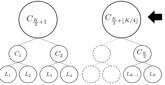
2.4 Example of a hierarchical copula model for a portfolio with 6 lines of business. 48

2.5 Hierarchical copula model used in Burgi et al. (2008). . . 49

2.6 Example of nested Archimedean copula. . . 49

2.7 Example of a HCM with six lines of business, three levels and five bivariate copulas. . . 54

3.1 Loss triangle with GLM equations of mean model. . . 60

3.2 Distributional visualization of the DGLM considered for the run-off triangle. 62

3.3 First level copula structure in the HCM. . . 63

3.4 Second level copula structure in the HCM. . . 64

3.5 Complete dependence structure of the HCM. . . 64

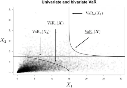
4.1 Univariate VaRα, bivariate lower and upper orthant VaR for Example 1. . 72

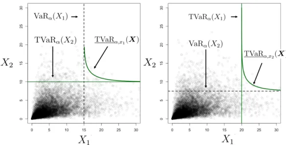
4.2 Set of two curves composing the bivariate lower orthant TVaRα,X(X) for

Example 1. . . 74

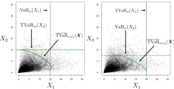
4.3 Set of two curves composing the bivariate upper orthant TVaRα,X(X) for

(10)

4.4 Univariate and bivariate VaRα and TVaRα intersection with proportional

allocation line for Example 1. . . 78

4.5 Zoom in of black box in Figure 4.4 to visualize intersection between uni-variate and biuni-variate risk measures with the proportional allocation line for Example 1. . . 79

5.1 Histograms of loss ratios for the 6 lines of business. . . 84

5.2 Behavior of the time series of the loss ratios by accident year for the auto-mobile industry of Ontario. . . 84

5.3 Goodness-of-fit measured through the Anderson-Darling and Kolmogorov-Smirnov test for the personal auto line of Ontario before the GEE approach (first row) and after the GEE approach (second row). . . 87

5.4 Time series of residuals before (first row) and after (second row) using GEE for the commercial auto line of Alberta. . . 87

5.5 Personal auto vs Commercial auto for Ontario . . . 88

5.6 Personal auto vs Commercial auto for Alberta . . . 88

5.7 Comparison of empirical copula for Alberta vs rank-based simulations of different copula families. . . 90

5.8 HCM structure by province. . . 92

5.9 HCM structure by copula family. . . 92

5.10 Historical data vs historical data with one simulation of loss ratios for personal auto in Atlantic Canada. . . 93

5.11 Historical data vs historical data with one simulation of loss ratios for commercial auto in Atlantic Canada. . . 93

5.12 100,000 Simulations of the reserves for the province of Alberta under the HCM. Univariate VaR (purple dotted lines) and TVaR (green straight lines) along with bivariate lower and upper orthant TVaR (green curved lines). Optimal couples shown with red dots. . . 96

(11)

List of Tables

1.1 Liability measurement approaches under IFRS 17. . . 5

2.1 General notation for a run-off triangle with loss ratios for the k-th line of business. . . 17

2.2 Some cases of the Tweedie family depending on the index parameter p. . . 24

2.3 Iman-Conover reordering algorithm example for the first node of depen-dence structure (HCM) from Figure 2.7. Inspired by examples in Arbenz et al. (2012).. . . 56

5.1 Goodness-of-fit and correlation test: p-values for marginal models. . . 85

5.2 Independence tests by province. The Cram´er-von Mises column shows the

p-values obtained. . . 89

5.3 Goodness-of-fit for copula models by province. . . 90

5.4 Goodness-of-fit for the second level of dependence: Alberta and Atlantic Canada. . . 91

5.5 Independence tests in the last node of the hierarchical copula model. . . . 91

5.6 Univariate VaR and TVaR at α = 99% in billions (CAD) for the six lines of business. . . 94

5.7 Risk adjustments corresponding to Table 5.6 for the univariate VaR and TVaR at α= 99% in billions (CAD) for the six lines of business. . . 95

5.8 Risk adjustments calculated through bivariate risk measures in billions (CAD) under different risk assumptions at a confidence level α = 99% for the HCM. . . 98

(12)

5.9 Cost of capital method disclosed by accident year in billions (CAD) for personal auto in Ontario assuming a cost of capital rate rt = 8% and

discount rate dt = 2%. . . 99

5.10 Risk adjustment for non-financial risks displayed in millions (CAD) for the six lines of business and equivalent confidence level for the VaR with two different assumptions for the cost of capital rate rt and discount rate dt. . . 100

A.1 Mean model - Accident year effects. . . 110

A.2 Mean model - Development Lag effects. . . 111

A.3 Dispersion submodel - Development lag effects. . . 112

A.4 Correlation parameter ρ estimated using GEE. . . 112

A.5 Index parameter p for the Tweedie distribution. . . 112

(13)

Introduction

Actuaries are interested in reserving the appropriate amount to cover for future claims, ensuring solvency for the insurer while, most importantly, protecting the insureds. The capital allocated to a reserve is disclosed on the financial reports of the insurance entities. New international financial reporting regulations have been set with the new International Financial Reporting Standards (IFRS 17) to homogenize and facilitate their interpreta-tion, making it simpler to compare insurance entities across jurisdictions.

Generalized linear models are commonly used in the industry to forecast future claims due to their accuracy and simple interpretation. In the recent actuarial literature, awareness to model the dispersion jointly with the mean has increased through double generalized linear models. Moreover, it is essential to verify that the assumptions of the statistical models are satisfied. Insurance portfolios are represented by multivariate distributions and due to the increasing computational power and development of the theory for copulas, modeling and measuring the risk associated with the multivariate distribution while accounting for dependence has become fundamental.

This thesis is structured as follows. In Chapter1, we discuss the new IFRS 17 framework for financial reporting, the capital requirements set by the insurance regulator in Canada and a justification for the proposed model. Chapter2explains the statistical and actuarial concepts needed to understand the model in Chapter 3. Chapter 4 describes the concept of reserving through univariate and multivariate risk measures. Furthermore, the cost of capital method is presented to account for a risk adjustment. Then, in Chapter 5 the model is applied to a dataset from the Canadian automobile industry.

(14)

Chapter 1

Background

In this chapter, basic insurance definitions are presented, along with laws and the entities responsible of regulating the insurance industry in Canada to justify the model suggested in this thesis.

An insurance contract or policy is issued by an entity called the insurer for exchange of a monetary consideration also known as a premium. The policy protects the owner of the contract, also called the insured or policyholder, against a possible unfavorable event with economic consequences. Specifically in this thesis, we are interested in Property and Casualty (P&C), an insurance entity that protects the policyholder from costs arising by loss or damage to tangible or intangible property. Examples of P&C insurance contracts include but are not limited to fire, marine, legal expenses and automobile insurance. The numerical results presented in Chapter5 are an application in automobile insurance.

In order to protect the policyholder, laws exist to regulate the financial management of the insurance companies through financial reporting and accounting standards. Laws regulating the insurance industry for Canada are found in the Insurance Companies Act Government of Canada (1991). The Insurance Companies Act states the Office of the Superintendent of Financial Institutions (OSFI) as the primary regulator of insurance companies with a federal charter in Canada. OSFI sets guidelines with regard to the capital and solvency of the insurer. The Insurance Companies Act also states that all

(15)

financial statements must be prepared in accordance with generally accepted accounting principles, the primary source of which is the Handbook of the Chartered Professional Accountants Canada. In May 2018, OSFI announced in OSFI (2018a) that IFRS 17 Insurance Contracts1 was endorsed by the Canadian Accounting Standards Board and thus, it is now incorporated into the Handbook.

It is of vital importance to highlight that capital requirements imposed by OSFI or other insurance regulatory entities in other jurisdictions serve a different purpose than for IFRS reporting. While a regulatory entity establishes principles in order to protect the pol-icyholder and ensure solvency by the insurer at all times, IFRS has the objective of creating comparable financial reporting across international boundaries for benchmarking purposes. Thus, in Section1.1 specific information is presented regarding the new IFRS international framework for financial reporting and in Section 1.2 we deal with capital allocation requirements set by the OSFI in Canada. In Section 1.3, we justify the model used throughout this thesis related to the capital requirements and the financial reporting framework.

1.1

Reporting - IFRS 17

Insurance Contracts

The International Accounting Standards Board (IASB), an independent international non-profit group of experts in accounting and financial reporting, issued IFRS 17 Insurance Contracts, a new accounting standard for insurance contracts in May 2017, superseding the current regulatory framework IFRS 4. IFRS 17Insurance Contracts establishes principles for the recognition, measurement, presentation and disclosure of insurance contracts.

IFRS 4 worked well reflecting national requirements because it allowed for different ac-counting practices. But having dissimilar standards across countries made it difficult for investors, analysts and decision makers to compare insurers’ results. IFRS 17 is in-tended to be the key towards a common international insurance accounting standardIASB

(16)

(2017a). The effective date of IFRS 17 has officially been set by the IASB to January 1st_,

20212, meaning March 31st, 2021 is the first quarter of reporting under IFRS 17.

Although in this thesis the numerical results presented in Chapter5 are from the Cana-dian industry and the capital requirement standards are considered under the CanaCana-dian regulator (OSFI), IFRS 17 is an international framework working under several jurisdic-tions, meaning the model described in Chapter 3can be applied in other countries while respecting the specific national capital requirements.

1.1.1

Measurement

Measurements under IFRS 17 seek to faithfully disclose the insurers’ obligations arising from the portfolios of insurance contracts. IFRS 17 establishes three approaches to mea-sure a liability depending on the duration (short and long term contracts), type of liability, and whether the contract depends on an underlying item. There are two types or classi-fications of liabilities under IFRS 17, liability for remaining coverage (LRC) and liability for incurred claims (LIC). LRC represents the unearned portion of risk from insurance contracts which are in force and LIC represent insurance events that already occurred but the claims have not been reported or have not been fully settled. Three measurement approaches and some examples of applicable contracts are presented in Table 1.1 which is adapted from CIA-CAS(2018). None of the measurement methods explained in what follows are mentioned in the superseded framework IFRS 4.

We are interested in P&C contracts, which under IFRS 17, can be measured with the General Model or with the PAA (as presented in Table 1.1). The General Model is the default approach for LIC because the horizon is usually more than one year. The PAA is an optional simplification which can apply for LRC if the duration of the contract is less or equal than one year (short-term contract). An example of a multi-year P&C contract is home insurance, where the insurer protects the policyholder against possible defects in the 2_{The IASB has proposed delaying the implementation of IFRS 17 by one year to 2022, subject to}

(17)

construction of a home. Most automobile insurance contracts are short-term given that the duration of the policies is for a one year period. Consequently, on initial recognition3, the measurement of the liabilities for remaining coverage is performed under the PAA.

General Model Premium Allocation Approach (PAA)

Variable Fee Approach (VFA)

Applicability Default approach To simplify short-term contracts (optional).

Direct Participation Con-tracts: where policy cash flows are linked to under-lying items.

•Life insurance •Most P&C •Segregated funds Examples of •Life annuities contracts •Unit-linked contracts

applicable •Universal life (UL) •Short-term •Index-linked UL contracts •Reinsurance contracts group contracts •Not applicable to P&C

•Multi-year P&C

Table 1.1: Liability measurement approaches under IFRS 17.

According to the PAA in paragraph 55 of IASB (2017b), the liability is measured on initial recognition as:

• The premiums,

• Minus acquisition cash flows (e.g. commissions paid to agents or taxation over the premiums),

• Plus or minus any amount arising from the derecognition (at the date of recog-nition of the insurance contracts) of prepayments, incurred expenses or any other acquisition cash flow the insurer pays or receives before the date of recognition.

P&C short-term contracts are accounted under the PAA which does not involve a risk ad-3_{Recognition (derecognition) is the addition (removal) of an asset or liability from the balance sheet.}

(18)

justment for non-financial risks component (described in Section1.1.2). However, events not settled during the duration of the contract sometimes occur. Thus, the cost of the insurance event for the insurer could extend for years. The unknown amount that will be paid in upcoming years is also known as unpaid claims liabilities for expired coverage under short-term contracts. Although the original insurance contracts were accounted for upon initial recognition with the PAA, the unpaid claim liabilities fall under the gen-eral measurement due to the duration of these liabilities, as mentioned in IAA (2018). Contrary to the PAA, the General Model requires a risk adjustment for non-financial risks (described in Section 1.1.2). Therefore, even for short-term contracts, the general approach is most of the time required in order to take into consideration the unpaid claim liabilities.

We highlight the importance of the unpaid claim liabilities which are formed of two impor-tant reserves known as the Incurred But Not Reported (IBNR) reserve and the Reported But Not Settled (RBNS) reserve. IBNR and RBNS are reserve accounts representing the amount of money the insurer has to set aside to fulfill future liabilities as consequence of the insurance contracts. Notation and methods to calculate the unpaid claim liabilities are described in Chapter2.

Since the unpaid claim liabilities or LIC fall under the General Model, we need to un-derstand the measurement requirements. The General Model establishes in paragraph 32 of IASB (2017b) that upon initial recognition, a group of insurance contracts should be measured as the sum of:

• The fulfillment cash flow (FCF), which include: – Estimates of future cash flows,

– An adjustment to reflect the time value of money and the financial risks related to the future cash flows,

– A risk adjustment for non-financial risk.

(19)

“The contractual service margin (CSM) represents the unearned profit the entity will rec-ognize as it provides services in the future” as stated in paragraph 38 of IASB (2017b). CSM applies for unexpired coverage (LRC) and it is not within the scope of this work.

1.1.2

Risk adjustment for non-financial risk

To calculate the unpaid claim liabilities that fall under the General Model within the IFRS 17 framework, in this section we describe the definition, specific characteristics and other considerations for the risk adjustment for non-financial risks. There exist non-financial risks that can arise from insurance contracts that all insurance entities share but there are risks that are entity specific. The shared non-financial risks are, as mentioned inIAA (2018),

• Model risks: in practice, the true model of the unpaid claim amounts is unknown, thus, the difference between the true model and the model used to estimate the FCF is known as model risk. Additionally, we rely on limited variables to predict the unpaid claim amounts, augmenting the model risk.

• Parameter risk: given that only a sample of the phenomena is observed, the es-timation of the parameters of the model could be biased or differ from the true parameters

• Process risk: assuming the model and parameters are correctly specified, the random nature of the phenomena can lead to a difference between the observed and estimated FCF.

Examples of entity specific non-financial risks for life insurance include mortality risk, lapse risk, etc. In this thesis, since we deal with automobile insurance (P&C), the en-tity specific non-financial risks considered are frequency and severity risks. Frequency and severity risks are the uncertainty associated to the number of claims and their cost, respectively.

(20)

1.1.2.1 Definition

As stated in paragraph 37 ofIASB(2017b), for the definition of a risk adjustment for non-financial risks,“An entity shall adjust the estimate of the present value of the future cash flows to reflect the compensation that the entity requires for bearing the uncertainty about the amount and timing of the cash flows that arises from non-financial risk.” Thus, the actuary shall exclude incorporating into the calculation of the risk adjustment financial risks and risks that do not arise from insurance contracts. Examples of the aforementioned risks are, but are not limited to, investment risk, credit risk, operational risk, interest rate risk and underwriting risk which are included in other sections of the financial reports.

The risk adjustment can be understood as the price assigned by the insurer for bearing the non-financial risks associated with the portfolio of insurance contracts, more specifically, the risks that arise from unfavorable outcomes on a long-term horizon. This assigned price has to meet the objective and characteristics described in the following Sections

1.1.2.3and 1.1.2.4.

1.1.2.2 Example

From paragraph B87 of IASB (2017b), “The risk adjustment for non-financial risk for insurance contracts measures the compensation that the entity would require to make the entity indifferent between:

• Fulfilling a liability that has a range of possible outcomes arising from non-financial risk; and

• Fulfilling a liability that will generate fixed cash flows with the same expected present value as the insurance contracts.”

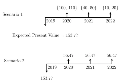
To improve the understanding of the indifference principle, we present a simplifying exam-ple. We use a time value of money diagram in Figure1.1, where we consider the following simplifying assumptions: an annual interest rate of 5%, the range of outcomes arising from the non-financial risks in the portfolio of insurance contracts, which are

(21)

equiproba-ble over a 3 year period, the insurer has no profit nor any other expense and we assume equal fixed cash flows.

Scenario 1

2020 2021 2022

2019

{100, 110} {40, 50} {10, 20}

Expected Present Value = 153.77

Scenario 2

2020 2021 2022

2019

56.47 56.47 56.47

153.77

Figure 1.1: Comparison of scenarios using a time value of money diagram.

In Figure 1.1, we can observe in Scenario 1 a liability with a range of outcomes arising from non-financial risk and in Scenario 2, using the same expected present value from the insurance contracts in Scenario 1, a liability that will generate fixed cash flows. Therefore, the risk adjustment is the price in excess of the 153.77 currency units that accounts for the uncertainty in Scenario 1 and thus, causing the insurer to be indifferent from selecting either of the scenarios.

1.1.2.3 Objective

“The objective of a risk adjustment is to provide a quantitative assessment of risk based on the entity’s risk preferences” IAA (2018). To meet the objective, the following elements mentioned inIAA (2018) can be considered in developing the adjustment:

• Risk preferences,

(22)

• The complexity of the probability or stochastic models,

• The ability to explain and quantify the risk adjustments in the context of financial statements.

1.1.2.4 Characteristics

The risk adjustment is a point estimate, not a range, and is stated in the same mone-tary terms as the other monemone-tary values in the entity’s financial statement IAA (2018). Paragraph B88 ofIASB(2017b) states that the risk adjustment for non-financial risk also reflects:

• “The degree of diversification benefit the entity includes when determining the com-pensation it requires for bearing that risk,

• Both favorable and unfavorable outcomes, in a way that reflects the entity’s degree of risk aversion.”

In paragraph B91 of IASB(2017b), it is stated that the estimation technique(s) used to determine the risk adjustment for non-financial risks are not specified. However, the risk adjustment should comply with the following characteristics:

Risks with respectively,

• Low frequency and high severity,

• Longer duration,

• Higher variance,

• Higher parameter uncertainty,

will result in a higher risk adjustment for non-financial risks than risks with respectively high frequency and low severity, shorter duration, lower variance and lower parameter uncertainty. Additionally:

(23)

of cash flows, will decrease (increase) the value of the risk adjustments for non-financial risks.

1.1.2.5 Disclosure

Once the risk adjustment for non-financial risks has been calculated with the appropriate technique(s) to reflect the entity’s view of compensation for bearing the uncertainty of the insurance contracts considering the objective and characteristics presented in Sections

1.1.2.3and 1.1.2.4, then, disclosure is required. More specifically, paragraph 119 of IASB (2017b) states that if the insurer uses a technique different from the Value-at-Risk4_,

commonly abbreviated as VaR (see Chapter 4 for definition) for determining the risk adjustment for non-financial risks, then, the insurer has to show the technique(s) used and disclose the corresponding level of confidence associated to the result obtained through the corresponding technique. For example, if the risk adjustment is set to X using the cost of capital method (described in Chapter 4) then the actuary has to disclose that X

is equivalent to the VaR at a α% confidence level.

1.1.2.6 Contrasts with Standards of Practice

The current accepted actuarial practice framework in Canada is established in a document called Standards of PracticeASB(2018) from the Actuarial Standards Board, established by the Canadian Institute of Actuaries (CIA). The Standards of Practice has a concept called Provision for Adverse Deviations (commonly known as PfAD) which measures the effect of uncertainty of the assumptions and data in determining the liability. The method to calculate PfAD can also be used to determine the risk adjustment but only if all the proper precautions are taking into account since both have different purposes. The following examples accompanied by a list that summarizes the contrasts between the PfAD and the risk adjustment will help understanding the important differences between the two concepts.

(24)

• Example A. Under IFRS 17, an insurer with a risk aversion policy has set the risk adjustment for non-financial risks to $10 million using the cost of capital method (described in Chapter 4),

• Example B. Following the Standards of Practice, the appointed actuary of an insurer might expect the interest rate to be 5% but assumed for the calculations a 4% interest rate. This difference in the interest rate could value the liabilities in $110 million and $100 million, respectively. Thus, the provision for adverse deviations is the difference of $10 million.

Even though the monetary value of the PfAD and the risk adjustment in Example A and B are exactly the same, we compare and summarize their differences with the following list:

• Objective: While the PfAD is a provision to account for uncertainty in the assump-tions of the liability estimation, the risk adjustment is meant to reflect the entity’s view of compensation for risk. In Example A, the risk preferences of the insurer were taken into consideration. Another insurer with the same group of insurance contracts could have set a higher risk adjustment to reflect the entity’s view for the compensation for bearing the uncertainty,

• Scope: The risk adjustment only accounts for uncertainty arising from the insurance contracts, contrary to the PfAD, which in Example B, clearly also accounts for uncertainty in financial risks,

• Responsible: Under the Standards of Practice, the entity responsible for the PfAD is the appointed actuary whereas IFRS 17 intends to involve management since the definition of the risk adjustment is associated with the entity’s view of compensation for bearing the uncertainty,

• Method: as stated in Section 1.1.2.4, the technique(s) to calculate the risk adjust-ment for non-financial risks are not specified under IFRS 17. Under the Standards of Practice the PfAD is the difference obtained from using more conservative

(25)

as-sumptions to protect the insurer for adverse deviations (hence, the name PfAD),

• Diversification Benefit: Under IFRS 17, the level of aggregation depends solely on the insurer’s view of diversification within an insurance portfolio. In other words, when considering similar risks, the level of aggregation to calculate the diversifi-cation benefit can be done at a line of business level (low level) or across entities among the same group (highest level). Under the Standards of Practice no ex-plicit consideration was given until 2017 where in section 2120, paragraph 07 was added. This paragraph states, “The provision resulting from the application of all margins for adverse deviations5_{, in addition to increasing the net liability, should be}

appropriate in the aggregate.” Thus, even if in practice it is considered (not often considered according to CIA (2018)), the diversification benefit would also involve financial risks, contrary to the IFRS 17 specifications.

• Disclosure: A entirely new requirement under IFRS 17 is to disclose the confidence level equivalent to the VaR technique (as described in Section 1.1.2.5).

1.2

Capital allocation - OSFI

The previous Section 1.1 deals with financial reporting for insurance contracts, which is managed by IFRS and applies to all IFRS jurisdictions. In this section, the regulatory principles set by OSFI are described and thus, the information presented is specifically for Canadian federally regulated insurers. These principles have the goal of ensuring an insurance entity maintains adequate capital levels in order to always be able to pay their liabilities to policyholders and creditors. The document Guideline A: Minimum Capital Test (MCT)OSFI(2018b) provides the framework within which OSFI assesses whether a P&C insurer maintains an adequate level of capital. The capital allocated with IFRS 17 needs to be compared with the capital levels set by OSFI since the latter is the minimum amount permitted by an insurance company in Canada.

(26)

OSFI sets a minimum amount of capital that needs to be available at all times to address and support insurance risks called minimum capital which works as an indicator for the regulator. If the insurer capital falls below this threshold, the continuity of the entity becomes questionable. To alert OSFI before the occurrence of this event, there exists a supervisory target capital providing a margin of 50% above the minimum capital. The target capital requirements has been set by OSFI in OSFI (2018b) to be the conditional tail expectation at a 99% level for insurance risk, over a period of one year or alternatively, if deemed not practical by an expert, the VaR at 99.5% confidence level (see Chapter 4

for a description of such risk measures). Thus, due to the 50% margin mentioned, the minimum capital becomes the target capital divided by 1.5.

The target capital requirement (TCR) is calculated as

TCR = Insurance + Market + Credit + Operational − Diversification

risk risk risk risk credit

In this thesis, we focus on the capital required for insurance risk, which corresponds to the risk that arises purely from the insurance contracts. Insurance risk breaks down as the following four components:

• Capital required for unpaid claims liabilities (or LIC),

• Capital required for premium liabilities (or LRC),

• Margin required for reinsurance ceded to unregistered reinsurers,

• Catastrophe reserves.

Unpaid claims according to OSFI have to be calculated by line of business. An insurer should not rely only on these regulatory capital measures but should conduct its Own Risk and Solvency Assessment (ORSA) OSFI (2018c) and, based on the entity’s risk composition, determine its particular capital requirements and establish Internal Capital Targets OSFI (2018d).

(27)

1.3

Justification of the copula model

In order to obtain the diversification benefit related to the aggregation and pooling of risks, it is necessary to apply appropriate statistical techniques. In the specific case of P&C, naturally offsetting product lines may not exist, contrary to products in life insurance that compensate with payout annuities where the insurer pays if the policyholder survives, and thus, mortality is offset by longevity as stated in IAA (2018). Therefore, in P&C, diversification benefits are available by aggregating types of commercial and personal products, through geographical dispersion of risk dependent on legislation Burgi et al. (2008) or by dependence strength measured with a distance-based method Cˆot´e et al. (2016).

IFRS 17 allows an entity to set the risk adjustment at a level of aggregation that rep-resents the compensation the entity requires for bearing the uncertainty regarding the liabilities. “For example, the risk adjustment might be set at the entity level, thus, incor-porating all diversification benefits in the organization aggregated across its product lines” as mentioned in IAA (2018). The use of this level of aggregation would produce a high level of diversification of risk, therefore, a small risk adjustment amount.

In order to comply with IFRS 17 and set the appropriate reserve amount to protect the policyholders under the requirements set by OSFI, we need a statistical model which can capture the characteristics established in this chapter and provide the risk adjustment for non-financial risks needed for the unpaid claim liabilities. An appropriate statistical method of risk aggregation is the hierarchical copula model reviewed in Chapter 2.

(28)

Chapter 2

Review of Actuarial and Statistical

Models

In order to calculate the risk adjustment for non-financial risks from IFRS 17, described in Section1.1 and to calculate the minimum capital required by OSFI to demonstrate finan-cial strength towards the policyholder and creditors described in Section1.2, this Chapter describes common actuarial and statistical models which are of use in the construction of the model presented in this thesis in Chapter3. First, we introduce the notation. Then, in Section2.2 the marginal distributions considered for each line of business are described. In Section 2.3, the multivariate model which accounts for the diversification benefit is presented, and finally, in Section 2.4, the simulation technique for the estimation of the unpaid claim liabilities is described.

2.1

Notation

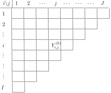
Claims can be presented graphically in an upper triangle array as in Table2.1, commonly known as a run-off triangle. This presentation can be done in two different ways, with cumulative claims Ci,j or incremental claims Ci,j − Ci,j−1, where Ci,0 = 0; the latter

(29)

{1,2, . . . , I} represents the accident year, j ={1,2, . . . , J}the development lag, and I, J

represent the last year of available information (data can also be measured by semester, quarterly or monthly). The development lag is the number of years between the occurrence of the accident and the date in which the final payment is made (closure of case).

To standardize claims and have comparable data, either premiums or volume (number of claims) are used for each line of business, depending on available information. In this thesis, the premiums are used to create what is known as a loss ratio. We denote the loss ratio for accident yeari, development lagj and for line of businessk as Y_i,j(k) and the premiums of accident yeari with p(_ik):

Y_i,j(k)=

C_i,j(k)−C_i,j(k)₋₁

p(_ik) . (2.1.1)

The superscript k = {1,2, . . . , K} denotes the line of business, where K is the total number of business lines available.

i\j 1 2 · · · j · · · J 1 2 .. . i Y_i,j(k) .. . .. . .. . I

Table 2.1: General notation for a run-off triangle with loss ratios for the k-th line of business.

Note that after each year that goes by, one diagonal is added to the loss triangle. Fur-thermore, in this thesis there is no explicit correction for inflation; it is assumed to be captured within the development lag factors.

(30)

2.2

Marginal distributions

2.2.1

Collective Risk Model

A common practice in the insurance industry is to use the collective risk model which provides a way to understand the aggregate loss as the sum of the individual claims. Following the notation from Klugman et al. (2008), let S be the random variable which represents the aggregate loss of a random number of claims N, of independent and iden-tically distributed random variables Xi, i = 1,2, . . . , n. In the insurance industry, N is

known as the frequency component andXi as the severity (risks also described in Section

1.1.2). Then, S has the following additive representation,

S =      0 N = 0, X1+X2+. . .+XN N >0 (2.2.1)

The collective risk model has the following independence assumption:

• Conditionally on N =n, N and the i.i.d. sequence Xi, i= 1,2, . . . , n are

indepen-dent.

N has to be a discrete count random variable and in the insurance context X follows a positive continuous random variable. In this thesis, a Poisson distribution is assumed for the count random variable and a gamma distribution for the severity.

2.2.2

Compound Poisson-Gamma distribution

The following definitions are useful in the construction of the objective distributionS. Definition 2.2.1. LetX be a positive continuous random variable with probability density function,

fX(x) =

βα_xα−1

Γ(α) e

(31)

where α, β > 0. Then, X is said to follow a gamma distribution with shape parameter α and rate parameter β and it is denoted X ∼ Gamma(α, β). A gamma distribution has moment generating function (m.g.f.) MX(t) =

1− t

β

−α

, for t < β.

Definition 2.2.2. Let N be a discrete random variable with support on the set of non-negative integers _N∪ {0} and probability mass function,

PN(n) =

e−λλn

n! , (2.2.3)

where λ >0. Then, N is said to follow a Poisson distribution with parameter λ and it is denoted N ∼ P oisson(λ). The moment generating function of a Poisson distribution is MN(t) = exp(λ(et−1)), for any t∈_R.

Theorem 2.2.1. (Klugman et al., 2008) Let S represent the aggregate loss from the collective risk model as presented in Section 2.2.1, with frequency N ∼ P oisson(λ) and severityX ∼Gamma(α, β), then the moment generating function of S is,

MS(t) = exp λ " 1− t β −α −1 #! , t < β. (2.2.4) Proof. MS(t) =E[eSt] =E[E[eSt|N]] = E[E[e(X1+X2+...XN)t|N]] i.i.d. =_E[_E[eXit_|_N_]N_{] =} E[MXN] =E[e Nlog(MX(t))_] =MN(log(MX(t))) = exp λ " 1− t β −α −1 #! .

Definition 2.2.3. A distribution S with m.g.f. of the form (2.2.4) is known as a Com-pound Poisson-Gamma distribution, denoted as S ∼CPG(λ, α, β).

(32)

2.2.3

Generalized Linear Models (GLM)

With the construction of our objective distribution S in Section 2.2.2 arises the need for a methodology to link the expected aggregate claim amounts with explanatory variables. Generalized linear modeling was introduced by McCullagh (1984), allowing to focus on the effects of explanatory variables, and generalizing the classical normal linear model by relaxing some of its restrictive assumptions. The GLM framework imposes for a random variableYi, fixed covariates Xi ∈Rp and for observations i={1,2, . . . , n}, that

g(_E[Yi|Xi]) = β0+

p

X

j=1

Xi,jβj =XiTβ, (2.2.5)

where g is a function called the link function, which defines the relationship between the linear predictors and the mean, and β is the vector of parameters that we want to estimate. If g is the identity function, we have a classic linear model. To simplify the notation of equation (2.2.5), the relationship is usually denoted by,

g(µi) =ηi, (2.2.6)

where µi is the conditional expected value of the response variable for observation i and ηi =XTi β is the additive relation of parameters and covariates.

GLMs rely on the following assumptions:

• Y1, Y2, . . . , Yn are conditionally independent givenX1,X2, . . . ,Xn,

• g must be monotonic and differentiable,

• Given the covariates Xi, the Yi are all distributed from the same member of the

exponential family.

Definition 2.2.4. LetY be a random variable that belongs to the exponential family, then Y has probability density function of the form,

fY(y;θ, φ) = exp   yθ−b(θ) a(θ) +c(y;φ)  , (2.2.7)

(33)

with canonical parameter θ, dispersion parameter φ and some specific functions a(·), b(·) and c(·). Furthermore, b(·) has to be twice differentiable and the random variable Y satisfies,

E[Y] =b0(θ), (2.2.8)

Var[Y] =b00(θ)a(θ). (2.2.9)

If the dispersion parameter φ is known, then (2.2.7) is referred to as a one-parameter exponential family. If φ is unknown, then, the distribution is part of the two-parameter exponential family or exponential dispersion family defined in the following section.

For the selection of the link functiong, it is a common practice in actuarial applications to use the log link because every covariate enters in the mean equation through a mul-tiplicative structure which allows to provide a simple interpretation of the parameters. Another convenient option is the canonical link function since it establishes a direct con-nection between the canonical parameter of the exponential family and the covariates, i.e.

θi =XTi β. But in some cases like the Gamma distribution, it allows the mean to vary on

the real numbers and thus, to enforce positive means the log link is used in this thesis.

2.2.4

Exponential Dispersion Family (EDF)

GLMs defined in2.2.3were originally developed for the exponential family. Then,Jørgensen (1997) introduced the exponential dispersion family by analyzing the error distribution of the GLMs. To draw a comparison between the exponential family and the exponen-tial dispersion family, we rewrite a random variable Y from the exponential family with density function as in equation (2.2.7), in its canonical parametrization:

fY(y;θ) = c(y) exp (yθ−κ(θ)), (2.2.10)

where θ remains the canonical parameter and κ(·) is the cumulant generator. Equation (2.2.10) lacks the parameter φ in contrast with equation (2.2.7) because for the usual

(34)

members of the exponential family (e.g. Normal, Poisson, Gamma and Binomial distri-bution), the dispersion parameter φ is assumed to be known. The definition for the EDF is as follows.

Definition 2.2.5. The distribution of a random variable Y is part of the exponential dispersion family if it has probability function of the form

fY(y;θ, φ) = c(y, φ) exp φ−1(yθ−κ(θ))

, (2.2.11)

where c(·,·) and κ(·) are given functions, θ ∈_R is the canonical parameter and φ >0 is the dispersion parameter. κ(·) is known as the cumulant function and is assumed to be twice differentiable.

Comparing the density function of the canonical parametrization of the exponential family (2.2.10) with the density function of the exponential dispersion family (2.2.11), we can deduce the latter is a generalization since they are equal up to an additional parameter, the dispersion parameterφ. The intention of the dispersion parameter, as interpreted by Madsen and Thyregod (2010), is to separate the mean from dispersion features like the sample size or common over-dispersion effects not related to the mean. Thus, it is a perfect fit for insurance claims because an assumption of the collective risk model (described in

2.2.1) is that conditionally on the number of claims, the frequency and the severity are independent.

The moment generating function of a random variable of the form (2.2.11) is

MY(t) = exp κ(θ+tφ)−κ(θ) φ . (2.2.12)

Following the notation from the original author Jørgensen (1987), any random variable

Y member of the EDF can be parametrized in terms of the location µ and dispersion φ

denoted as Y ∼ ED(µ, φ). The random variable Y has first moment _E[Y] = µ = κ0(θ) and variance Var[Y] = φV(µ), where V(µ) = κ00(θ) as presented in Jørgensen (1987). The function V(µ) is known as the variance function and captures the mean-variance relationship of the data as it is explicitly seen for the Tweedie family in Section2.2.4.1.

(35)

Another generalized concept is the residual sum of squares from the analysis of variance, for a member of the exponential dispersion family, it is called analysis of deviance and is equivalent to sums of unit deviancesJørgensen (1997).

Definition 2.2.6. A function d: Ω→_R is called a unit deviance if it satisfies

d(y;y) = 0 ∀y∈Ω

and

d(y;µ)>0 ∀y6=µ.

where Ω is the domain of the parameter µ.

The unit deviancedcan be understood as a measure of the distance fromyto the meanµ. Therefore, to analyze the dispersion features, it is necessary to calculate the unit deviances from the estimated mean. Additionally, with the unit deviance a random variableY from the exponential dispersion family can be reparametrized in the standard form,

fY(y;θ, φ) =c(y, φ) exp φ−1d(y;µ)

. (2.2.13)

Once the mean and dispersion have been estimated for different lines of business, in this thesis, the following theorem is essential to homogenize and study the dependence structure.

Theorem 2.2.2. If Y ∼ED(µ, φ) for some µ∈_R, we have

Y −µ p φV(µ) d − →N(0,1) as φ→0. (2.2.14)

P roof.Refer to Jørgensen (1997).

Theorem 2.2.2 shows that any member of the EDF is asymptotically normal for a small dispersion parameterφ.

(36)

2.2.4.1 Tweedie family

The Tweedie family, in honor of Tweedie (1984), is a member of the EDF where the variance function is of the form,

V(µ) =µp, (2.2.15)

for some indexp∈(−∞,0]∪[1,∞)1_{. A random variable of the Tweedie family is denoted}

Y ∼T Wp(µ, φ). Index Distribution p= 0 Normal p= 1 Poisson p∈(1,2) Compound Poisson-Gamma p= 2 Gamma p= 3 Inverse Gaussian

Table 2.2: Some cases of the Tweedie family depending on the index parameter p.

Table 2.2 shows how some very well known distributions are part of the Tweedie family. We pay special interest to the case where p ∈ (1,2). For p = 1, we have a Poisson distribution, which is discrete, and for p = 2 we have a continuous Gamma distribution. When p ∈(1,2) the distribution is mixed, continuous for positive values with a point of mass at zero, and as p→2, the distribution starts losing the point of mass. This mixed domain makes it very relevant for actuarial analysis, given that for certain years, specially several years after the accident year, the claims converge to zero as the development lag increases, and in some cases, is exactly zero.

To obtain the probability density function and the moment generating function of a 1_{The case} _p_∈₍₀_,_{1) has been shown by}_Jørgensen _{(1997) to have null variance for some cases of the}

canonical parameter making it a degenerate distribution and thus, concluding there are no members of the Tweedie family for these values ofp.

(37)

Tweedie distribution, we use the property of the EDF where V(µ) = κ00(θ) and the procedure described by Dunn and Smyth (2004). Thus, the canonical parameter θ is obtained by integrating the following differential equation and setting the constant equal to zero. µp =κ00(θ) = ∂µ ∂θ

Z

1 µpdµ=

Z

_∂θ ∂µ ⇒θ =          µ1−p 1−p p6= 1, logµ p= 1. (2.2.16)

And the cumulant function κp(θ) (with subscript p to denote the functional dependence

on the index) is obtained by integrating κ0_p(θ) =µwith respect to θ:

κp(θ) =              1 2−p((1−p)θ) 2−p 1−p p6={1,2}, eθ _p_{= 1}_, −log(−θ) p= 2. (2.2.17)

Thus, to obtain the connection between the Tweedie family (member of the EDF) with a CPG distribution, we substitute the canonical parameter (2.2.16) and the cumulant function (2.2.17) (whenp6={1,2}) into the moment generating function ofY ∼ED(µ, φ) shown in equation (2.2.12), MY(t) = exp 1 φ 1 2−p (µ1−p+ (1−p)φt)12−−pp −µ2−p . (2.2.18)

Then, Quijano Xacur (2011) proved the existence of Tweedie families for p ∈ (1,2) and shows that they are equivalent to a CPG(λ, α, β) distribution with the following trans-formations, λ= 1 φ µ2−p 2−p, α=− 2−p 1−p, β =− 1 φ µ1−p 1−p. (2.2.19)

(38)

Then, the moment generating function (2.2.18) becomes: MY(t) = exp   (µ1−p + (1−p)φt)−α φ(2−p) −λ   = exp λ " 1− t β −α −1 #! . (2.2.20)

Finally, we have showed the connection between the CPG distribution and the Tweedie family with p∈ (1,2) through the moment generating function by showing that (2.2.12) is equal to (2.2.20), provided the appropriate transformations (2.2.19) are used.

Another important result with actuarial applications from Jørgensen (1997) is the scale invariance of the Tweedie family,

Theorem 2.2.3. Let Y ∼TWp(µ, φ), then

cY ∼T Wp(cµ, c2−pφ). (2.2.21)

Proof. Refer to Jørgensen (1997).

Theorem 2.2.3 is fundamental to homogenize the data and sample from the Tweedie family as done in Section 2.4.1 when the dispersion parameter φ is assumed constant across observations. In this thesis, a GLM is used to estimate the dispersion parameter and therefore, another approach is taken.

Definition 2.2.7. The probability density function of a Tweedie random variable Y ∼ TWp(µ, φ) is of the form, fY(y;µ, φ, p) = a(y;φ, p) exp   1 φ  y µ1−p 1−p− µ2−p 2−p     (2.2.22) where a(y;φ, p) = ∞ X r=1   φp−1y` (2−p)(p−1)`   r 1 r!Γ(r`)y, `=− 2−p 1−p.

Thus, the point of mass at zero has probability given by,

fY(0;µ, φ, p) = exp  − µ 2−p φ(2−p)  .

(39)

2.2.5

Double Generalized Linear Models (DGLM)

We have introduced GLMs in Section 2.2.3 to link the expected insurance claims with explanatory variables. Then, by analyzing the error distribution of the GLMs Jørgensen (1997) introduced the EDF, as described in Section2.2.4. The EDF led us to the Tweedie family in Section2.2.4.1as a link with the CPG distribution under the appropriate trans-formations. In this section, to account for the dispersion features we study DGLMs. These double generalized linear models allow the mean and the dispersion to be modeled simultaneously using GLMs. DGLM handles the case where only the aggregate claims is available but the number of claims has not been recorded or is unreliable, seeSmyth and Jørgensen(2002). Furthermore, DGLM is a more flexible model since we add a new set of parameters to be estimated for the dispersion and thus, should be used carefully to avoid overfitting. Research in actuarial science likeSmyth and Jørgensen (2002); Boucher and Davidov (2011), and more recently Andersen and Bonat (2017); Smol´arov´a (2017) have highlighted the importance of modeling the mean and dispersion structures for claims reserving.

Introduced bySmyth(1989), the simultaneous estimation for the mean and dispersion for a Tweedie distribution is possible due to the statistical orthogonality of the parametersφ

and pto µ, as explained in what follows.

Definition 2.2.8. The parameter orthogonality introduced byCox and Reid(1987), states that if we partition the parameter vector of interest θ = (µ, φ, p) into θ1 = µ and θ2 =

(φ, p), and the information matrix of the corresponding log-likelihood L satisfies,

E  − ∂ 2_L ∂θ1∂θ2 ;θ  = 0, (2.2.23)

then, θ1 and θ2 are said to be locally orthogonal.

Equation (2.2.23) implies mainly that the maximum likelihood estimates ofθ1 andθ2 are

(40)

2.2.5.1 Estimation of DGLM

In this section, we explain the estimation procedure used to obtain the parameters of the mean model and the dispersion submodel for independent observations from a Tweedie distribution through a DGLM. The algorithm procedure described in what follows serves as a building block for algorithms in the presence of correlation between observations as illustrated in subsequent sections. The procedure consists in an alternating scheme presented inSmyth(1989) where the dispersion is assumed to be known when estimating the mean and then, the mean is assumed to be known when estimating the dispersion. The alternation is possible due to the parameter orthogonality (Definition 2.2.8) of the parameter vector. The estimation of the index parameter p, the power of the variance function for a member of the Tweedie family, is a more difficult problem than estimating

φ or µ. Most authors using Tweedie densities have taken p to be specified a priori as in Dunn and Smyth(2004). In other words, p is fixed in the interval (1,2) to guarantee the existence of the connection with the CPG distribution, and then, the process to obtain the maximum likelihood estimates ofµandφbegins. The process is repeated with several values of the indexpuntil the likelihood function is maximized within a given threshold. This procedure to estimate µand φ is explained in what follows.

For observations y ={y1, y2, . . . , yn}, from the random variable Yi|Xi ∼TWp(µi, φi) we

assume a DGLM with the following equations:

g(µi) =XiTβ, g(φi) = ZiTγ, (2.2.24)

where X, Z are the matrix of fixed covariates for the mean and dispersion submodel, re-spectively. The same log-link function g(x) = log(x) is used for both GLMs (reasons ex-plained in Section2.2.3) andβ,γare the parameter vectors we wish to estimate. Further-more, to simplify notation we denote the vector of mean parameters as µ={µ1, . . . , µn}

and the vector of dispersion parameters asφ={φ1, . . . , φn}. Initially, we assume the

(41)

β. We denote the log-likelihood function as, L(β|y,γ, p) = n

X

i=1 logfY(yi;µi, φi, p). (2.2.25)

We proceed to establish a recursive algorithm to estimate β as presented in Hardin and Hilbe(2013). The estimates of the parameter vector β are the solution of the estimating equation given by,

∂L

∂β= 0. (2.2.26)

The solution denoted asβ∗ can be obtained by a Taylor series expansion,

∂L ∂β(β ∗ )−(β−β∗) ∂2_L ∂β∂βT +. . .= 0, (2.2.27)

by solving for β∗ and substituting the expected value of the Hessian matrix given by,

−_E   ∂2L ∂β∂βT  =XTW X. (2.2.28)

Results in the weighted ordinary least squares equation for iterationk+ 1,

β(k+1) = (XTW X)−1XTWz, (2.2.29)

whereW is the diagonal matrix of weights. To introduce W, we first denote diag(wi) as

the notation to represent a diagonal matrix whose entries are the elements{w1, . . . , wn}.

Consequently, the weights to estimate the parameters of the mean model are,

W = diag      ∂g(µi) ∂µ   −2 1 Var(yi)   = diag µ2_i−p φi , (2.2.30)

where Var(yi) = φiV(µi), µi = g−1(XiTβ(k)) and the right side equation is obtained

through the log-link function and the Tweedie distributional assumption with variance function of the form (2.2.15). The vector z from equation (2.2.29) has components,

zi = ∂g(µi) ∂µ (yi−µi) +g(µi) = yi−µi µi + logµi. (2.2.31)

(42)

After estimating the parameters of the mean model β, we proceed to estimate the pa-rameters of the dispersion submodel γ. As stated in Section 2.2.4, from the theory of dispersion models by Jørgensen (1997), the unit deviance is the equivalent of the sum of squares in analysis of variance. The unit deviance 2.2.6 for the Tweedie family is given by, di(yi;µi) =              2  yi y1_i−p−µ1_i−p 1−p − y_i2−p−µ2_i−p 2−p   yi 6= 0, 2 µ2_i−p 2−p yi = 0. (2.2.32)

By assuming the mean parameters β are fixed, Smyth (1989) showed that the log-likelihood given in equation (2.2.25) can be reparametrized in terms of the unit deviance, as done with equation (2.2.13) to obtain the standard form, causing the dispersion sub-model to have the form of a GLM with observations di, canonical parameter φi and

dispersion parameter 2. Thus, analogous to the mean model with observations yi and

canonical parameterµi, we use the unit deviance as the response vector of the dispersion

submodel.

Furthermore,Smyth and Verbyla (1999) showed that di ∼φiχ21 approximately as φi →0

with the saddlepoint approximation (refer to Jørgensen (1997) for more on the saddle-point approximation). Assuming a gamma distribution instead of a chi-square simplifies the procedure for the weight matrix of the dispersion submodel as shown in what fol-lows. This assumption is possible given that the χ2₁ distribution is a special case of the gamma distribution (2.2.1), therefore, a gamma GLM is fitted for the dispersion sub-model. Maximum likelihood estimators for variance parameters in regression models are generally biased, thus, a restricted maximum likelihood (REML) approach is used as in Smyth and Verbyla (1999) to adjust for degrees of freedom and produce estimators that are approximately unbiased.

Consequently, the unit deviances (2.2.32) are calculated and the parameters for the dis-persion submodel γ are obtained by using the same technique as for the mean model: Taylor series expansion forL(γ|y,β, p), substitute expected value of Hessian matrix and

(43)

thus, for iteration k+ 1 the weighted ordinary least squares equation for the dispersion submodel is,

γ(k+1) = (ZTWdZ)−1ZTWdzd, (2.2.33)

where Wd is the matrix of weights for the dispersion submodel using the same notation

asSmyth and Jørgensen (2002). The matrix Wd is given by,

Wd = diag      ∂g(φi) ∂µ   −2 1 2V(φi)   . (2.2.34)

Since we are fitting a gamma GLM, member of the Tweedie family with p = 2 (refer to Table 2.2), the variance function becomes V(φi) = φ2i. Thus, the weight matrix (2.2.34)

simplifies to a diagonal matrix with entries 1₂. Furthermore in equation (2.2.33), the vector

zd has the same structure as equation (2.2.31) but with response di. A REML approach

is used asSmyth and Jørgensen(2002) to correct for the bias of the maximum likelihood estimators for the variance parameter as mentioned in Section 2.2.5. The dispersion submodel is modified with,

γ(k+1) = (ZTW_d∗Z)−1ZTW_d∗z_d∗, (2.2.35) where W_d∗ = diag   1−hi 2  , z ∗ d = d∗_i −φi φi + logφi. (2.2.36)

The modified responses ared∗_i = di

1−hi andhi are the diagonal elements of the projection

matrix H, known as leverages from the mean model. The projection matrix H is given by,

H = diag(hi) = W1/2X(XTW X)−1XTW1/2. (2.2.37)

This REML approach is possible because of the extension made byCox and Reid (1987) and the simplifications on the convergence algorithm provided byLee and Nelder(1998).

(44)

2.2.5.2 DGLM estimation algorithm

To summarize, the estimation algorithm for the DGLM is as follows:

1. Set initial values µ(0)_i =yi, φ

(0)

i = 1,

2. For iteration k, obtainβ(k) _{with the equation (}_2.2.29_),

3. Calculate the unit deviancesdi with equation (2.2.32),

4. Obtain γ(k) with equation adjusted for the dispersion submodel (2.2.35) using the REML approach,

5. Calculate the maximum likelihoodL(y, p,µ(k),φ(k)) with the estimated parameters,

6. Set k=k+ 1 and repeat steps 2-5 until convergence.

2.2.6

Goodness-of-fit

The goal is to determine a model that is good enough for the marginal distributions to continue with the modeling procedure. We have to remember that“All models are wrong, but some models are useful.”2

A model deemedgood enough in this thesis is defined as a marginal model which will not reject the null hypothesis H0: the data came from a population with the stated model.

This is done through the Kolmogorov-Smirnov and Anderson-Darling tests to assess the fit on the center and tails of the distribution, respectively. The tests are defined as follows,

2.2.6.1 Kolmogorov-Smirnov (K-S)

For a random variableX and independent observations {x1, . . . , xn} fromX, letFn(x) =

1

n n

X

i=1

1(xi ≤ x) be the empirical cumulative distribution function, where 1(A) denotes

the indicator function which is set to 1 ifA occurs and zero otherwise. Additionally, let 2_{Usually attributed to George Box.}

(45)

F(x) be the model cumulative distribution function. Then, the statistic of the K-S test is calculated as,

D = sup

x

|Fn(x)−F(x)|. (2.2.38)

The model distribution functionF(x) is assumed to be continuous over the relevant range Klugman et al. (2008).

2.2.6.2 Anderson-Darling (A-D)

The test is similar to the Kolmogorov-Smirnov test but it uses a different measure of the distance between the two cumulative distribution functions. The test statistic is

A2 =n

Z

1

0

(Fn(x)−F(x))2

F(x)(1−F(x))f(x)dx. (2.2.39)

The Anderson-Darling test assesses whether the estimated model has a good fit close to the tails of the distribution. This can be seen in the denominator of the statistic; asF(x) gets closer to 0 and 1, the quotient reaches its maximum value.

The combination of the Kolmogorov-Smirnov test in Section 2.2.6.1 and the Anderson-Darling test in Section2.2.6.2ensures that the center and the tails of the fitted distribution are being assessed statistically.

2.2.7

Generalized Estimating Equations (GEE)

An important inspection for a fitted GLM is a residual plot in order to verify the indepen-dence assumption of the response variable given the fixed covariates as stated in the GLM Section2.2.3. For the loss ratioYi,j and the vector of fixed covariatesXi,j, it is reasonable

to suspect dependence between Yi,j|Xi,j and the loss ratio of the next development lag Yi,j+1|Xi,j+1. To address the issue when there is correlation between observations, GEE

suggest a way to estimate efficient parameters with the same concepts of a GLM model. Thus, a two-stage estimation method is proposed in this section by first estimating the

(46)

DGLM from Section 2.2.5 and then, to account for correlation, apply the estimation of the GEE presented in what follows. An example of claims reserving with GEE is men-tioned inHudecová and Peˇsta(2013) and this problem applied to non-life insurance data is mentioned in Smolárová (2017), but there are differences in this thesis regarding to the correlation estimator presented in what follows and the estimator of φ given that we consider a DGLM, compared to the moment estimator applied inSmolárová (2017).

GEE is a anad hoc method which can make it unattractive for some researchers. There are several research articles dealing with GLM models for non-life insurance, e.g. Shi and Frees (2011) and Cˆot´e et al. (2016), where correlation is not an issue raised by the authors. The usual application of GEE is in biostatistics, where the correlation is assumed for each subjectibetween the differentj measurements. The concepts are borrowed from this field and adapted to our context to capture the correlation for every accident year

i between the different j development lags. The theory is also developed to account for unbalanced data which is exactly the case for a loss triangle given that for every accident yeari, there is exactly one less development lagj due to the triangular nature of the data as it can be seen in what follows. First, we introduce the linear correlation considered for the generalized estimating equations.

Definition 2.2.9. For two square integrable random variables X and Y, Pearson’s cor-relation is defined as,

ρ(X, Y) = E

(XY)−_E(X)_E(Y) p

Var(X)Var(Y) . (2.2.40)

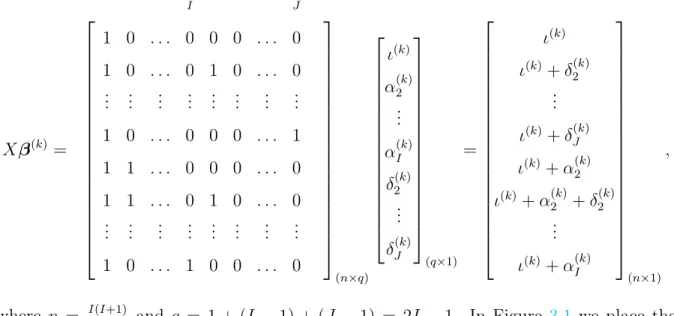
The correlation parameterρ is an additional parameter for the marginal distributions as it is described in what follows. The loss ratios for accident year i = {1,2, . . . , I} are grouped in a vector to ease the notation as in Figure 2.1,

(47)

Figure 2.1: Vectorial notation of loss ratios for GEE.

Thus, from Figure2.1, the random vectorYi ={Yi,1, . . . , Yi,ni}corresponds to the vector of

ni loss ratios with each component distributedYi,j|Xi,j ∼TWp(µi,j, φi,j) for accident year i, development lagj and correlation parameterρwhich is explained in what follows. The mean vector ofYi isµi ={µi,1, . . . , µi,ni}and has dispersion vector φi ={φi,1, . . . , φi,ni}.

The following results and notation are taken and adapted from Liang and Zeger (1986). Let X, Z be the same matrices of fixed covariates for the mean model and dispersion vector submodel, respectively, as in Section 2.2.5.1. The conditional variance matrix of the random vector is denoted Vi = Var [Yi|Xi]. The following generalized estimating

equation obtained fromLiang and Zeger(1986) corresponds to the weighted least squares estimator, which ensures the estimator of β to remain consistent,

ni

X

i=1 DT_i V_i−1(Yi−µi) = 0, (2.2.41) whereDi = ∂µi

∂β is a matrix of derivatives with dimension (ni×q),βthe parameter vector

of dimensionq and variance matrixVi =A

1/2

i Ri(ρ)A

1/2

i , where the matrixAi is presented

in what follows. The variance matrix Vi of dimension (ni ×ni) is key to capture the

correlation between observations. The diagonal matrix Ai is given by,

Ai =         φi,1V(µi,1) 0 . . . 0 0 φi,2V(µi,2) . . . 0 .. . ... . .. ... 0 0 . . . φi,niV(µi,ni)         (n×ni) , (2.2.42)

(48)

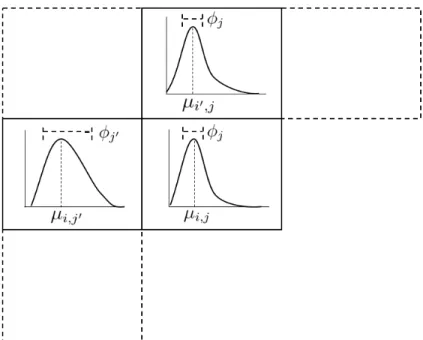
where the elementsV represent the variance function of the Tweedie family with equation (2.2.15). Furthermore, Ri(ρ) is the correlation matrix of the random vector Yi|Xi and in this thesis, we assumed the correlation matrix Ri(ρ) to be functionally related to the

scalar ρ which can be easily extended to be a vector depending on the independence assumptions. If the correlation matrix Ri(ρ) = Ini, where Ini is the identity matrix of

dimension (ni ×ni), then independence is assumed and the model is equivalent to the

normal GLM estimation. Common correlation matrices can be found inHardin and Hilbe (2013) with their respective estimators. In this thesis, an autoregressive model of order 1 or AR(1), is used to minimize the number of estimated parameters while providing a reasonable correlation matrix. An AR(1) assumes cor(Yi,j, Yi,j0|X_i,j,X_i,j0) = ρ|j−j

0_|

. Thus, the further apart the observations are in time, a smaller correlation is assumed. The correlation matrix for claims in accident yeari, has the form,

Ri(ρ) =            1 ρ ρ2 _{. . . ρ}ni−1 ρ 1 ρ . . . ρni−2 ρ2 _ρ ₁ _{. . . ρ}ni−3 .. . ... ... . .. ... ρni−1 _ρni−2 _ρni−3 _{. . .} ₁            (ni×ni) (2.2.43)

The correlation matrix in (2.2.43) assumes independence across accident years but for a given accident year, loss ratios are dependent between development lags. A parallel can be drawn between the general estimating equation (2.2.41)