Dynamic Rule Covering
Classification in Data Mining with
Cyber Security Phishing
Application
Issa Mohammad Qabajeh
Submitted in partial fulfilment of the requirements for the
degree of Doctor of Philosophy
at De Montfort University
Faculty of Technology
School of Computer Science and Informatics
Centre for Computational Intelligence
ACKNOWLEDGMENTS
First and foremost, I thank God for granting me the strength, patience,
good health, and ability to pursue this goal in my life.
I would like to express my deep thanks and gratitude to my supervisors
Prof. Francisco Chiclana and Prof. Fadi Thabtah for their continuous
support and everlasting encouragement during the long journey of my
PhD study in the United Kingdom. My thesis would not have been possible
without the guidance and the assistance of my supervisors who contributed
to the completion of this study.
My sincere thanks go to Dr. Jenny Carter for her support in allowing me
to further enhance my academic experiences through teaching modules and
supervising master students at De Montfort University.
My thanks should also be extended to my family throughout the past four years.
Very special thanks to my wife Neda’a. Her patience, encouragement and
support over the period of study in UK made things much easier than
expected.
Many thanks also go to my children who endured my absence and have always
been granting me their love and support.
Finally, I would like also to thank all my friends especially; Sadir,
Muhannad, Mohammad, and Ayad and all of my colleagues in the Centre
for Computational Intelligence who support me during my study.
DEDICATION
My thesis is dedicated to:
The souls of my late father, mother, sisters, and brothers, especially
my brothers who have passed away during the last two years of my
PhD. Study, Mahmoud, Abdlmajeed, and Jamal, truly I missed all
of them, God bless them all.
My brothers who have guided, mentored, and supported me during
the journey of my study, especially Abdlmuhdi, Abdlmonhem,
Samir, and Ziad, they are faithful brothers.
My wife Neda’a, for her continuous cheer on, patience and
empathy, she is my true supporter.
My children who have endured my absence in the UK; Dima, the
family mentor; Rand, the family active planner; Shahed, the family
loyal assistant; Amin, the gorgeous hero; and Malak, the lovely
butterfly, all of you my motivators. Love you all!!
Publications
Most of the chapters in this thesis have been published or submitted for publication in refereed international journals or conferences. The published papers are shown below. Additionally, there are two more journal papers under review.
Journals
• Qabajeh I., Thabtah F., Chiclana F. (2015) Dynamic Classification
Rules Data Mining Method. Journal of Management Analytics.Volume 2, Issue 3, pp. pages 233-253. Wiley.
• Thabtah F., Qabajeh I.., Chiclana F. (2016B.) Constrained dynamic rule induction learning. Expert Systems with Applications 63, 74-85.
• Qabajeh I. Thabtah F. Chiclana F. (2017) Understanding and Preventing Phishing: A recent Review. Journal of Information Security and Applications (Under Review)
Conferences
• Qabajeh, I. and Thabtah, F., 2014, December. An Experimental Study
for Assessing Email Classification Attributes Using Feature Selection Methods. In Advanced Computer Science Applications and Technologies (ACSAT), 2014 3rd International Conference on (pp. 125-132). IEEE.
• Qabajeh, I., Chiclana, F. and Thabtah, F., 2015, November. A
classification rules mining method based on dynamic rules' frequency. In Computer Systems and Applications (AICCSA), 2015 IEEE/ACS 12th International Conference of (pp. 1-7). IEEE.
ABSTRACT
Data mining is the process of discovering useful patterns from datasets using intelligent techniques to help users make certain decisions. A typical data mining task is classification, which involves predicting a target variable known as the class in previously unseen data based on models learnt from an input dataset. Covering is a well-known classification approach that derives models with If-Then rules. Covering methods, such as PRISM, have a competitive predictive performance to other classical classification techniques such as greedy, decision tree and associative classification. Therefore, Covering models are appropriate decision-making tools and users favour them carrying out decisions.
Despite the use of Covering approach in data processing for different classification applications, it is also acknowledged that this approach suffers from the noticeable drawback of inducing massive numbers of rules making the resulting model large and unmanageable by users. This issue is attributed to the way Covering techniques induce the rules as they keep adding items to the rule’s body, despite the limited data coverage (number of training instances that the rule classifies), until the rule becomes with zero error. This excessive learning overfits the training dataset and also limits the applicability of Covering models in decision making, because managers normally prefer a summarised set of knowledge that they are able to control and comprehend rather a high maintenance models. In practice, there should be a trade-off between the number of rules offered by a classification model and its predictive performance. Another issue associated with the Covering models is the overlapping of training data among the rules, which happens when a rule’s classified data are discarded during the rule discovery phase. Unfortunately, the impact of a rule’s removed data on other potential rules is not considered by this approach. However, When removing training data linked with a rule, both frequency and rank of other rules’ items which have appeared in the removed data are updated. The impacted rules should maintain their true rank and frequency in a dynamic manner during the rule discovery phase rather just keeping the initial computed frequency from the original input dataset.
based on Covering and rule induction, that we call Enhanced Dynamic Rule Induction (eDRI), is developed. eDRI has been implemented in Java and it has been embedded in WEKA machine learning tool. The developed algorithm incrementally discovers the rules using primarily frequency and rule strength thresholds. These thresholds in practice limit the search space for both items as well as potential rules by discarding any with insufficient data representation as early as possible resulting in an efficient training phase. More importantly, eDRI substantially cuts down the number of training examples scans by continuously updating potential rules’ frequency and strength parameters in a dynamic manner whenever a rule gets inserted into the classifier. In particular, and for each derived rule, eDRI adjusts on the fly the remaining potential rules’ items frequencies as well as ranks specifically for those that appeared within the deleted training instances of the derived rule. This gives a more realistic model with minimal rules redundancy, and makes the process of rule induction efficient and dynamic and not static. Moreover, the proposed technique minimises the classifier’s number of rules at preliminary stages by stopping learning when any rule does not meet the rule’s strength threshold therefore minimising overfitting and ensuring a manageable classifier. Lastly, eDRI prediction procedure not only priorities using the best ranked rule for class forecasting of test data but also restricts the use of the default class rule thus reduces the number of misclassifications.
The aforementioned improvements guarantee classification models with smaller size that do not overfit the training dataset, while maintaining their predictive performance. The eDRI derived models particularly benefit greatly users taking key business decisions since they can provide a rich knowledge base to support their decision making. This is because these models’ predictive accuracies are high, easy to understand, and controllable as well as robust, i.e. flexible to be amended without drastic change. eDRI applicability has been evaluated on the hard problem of phishing detection. Phishing normally involves creating a fake well-designed website that has identical similarity to an existing business trustful website aiming to trick users and illegally obtain their credentials such as login information in order to access their financial assets. The experimental results against large phishing datasets revealed that eDRI is highly useful as an anti-phishing tool since it derived manageable size models
when compared with other traditional techniques without hindering the classification performance. Further evaluation results using other several classification datasets from different domains obtained from University of California Data Repository have corroborated eDRI’s competitive performance with respect to accuracy, number of knowledge representation, training time and items space reduction. This makes the proposed technique not only efficient in inducing rules but also effective.
Table of Contents
Chapter One: Introduction………..1
1.1 Introduction... ...1
1.2 Motivation ... ...2
1.3Covering Induction Process and Related Definitions……….…5
1.4Thesis Research Issues ... 6
1.4.1 Generic Issues.. ... 7
1.4.2 Domain Specific Issues...11
1.5 Thesis Structure ...13
Chapter Two: Covering and Induction Approaches in Classification...14
2.1 Introduction ...15
2.2 The Classification Problem and Its Variations... 16
2.3 Learning Strategies in Classification ... 19
2.3.1 Divide and Conquer ... 19
2.3.2 ID3 Decision Algorithm...21
2.3.3 Separate and Conquer... 22
2.4Common Covering and Induction Algorithms... 25
2.4.1 PRISM Algorithm and its Successors………...……….….. 25
2.4.2Incremental Reduced Error Pruning and its Successors………...………...…30
2.4.2.1Reduced Error Pruning (REP)……….………..….. 30
2.4.2.2Incremental Reduced Error Pruning (IREP)………..……. 31
2.4.2.3RIPPER and Other Alternative Algorithms………..….. 33
2.4.3Rough set Theory Induction Algorithms………35
2.4.4 CN2 Algorithm………...37
2.4.5First Order Inductive Learner (FOIL)………39
2.4.6Instance Based Learning Rule Classifiers………....40
2.4.7One Rule and RIDOR Algorithms ………..41
2.4.8Hybrid Classification Rules……….... 42
2.5 Other Common Classical Non-Rule Approaches... 43
2.5.1 Probabilistic Models... 44
2.5.2 Association Rule-based Classification... 45
2.5.3 Support Vector Machine...45
2.5.4 Boosting ...46
2.5.5 Neural Network ... 46
2.6 Chapter Summary ... 47
Chapter Three: A New Dynamic Rule Induction Approach... 48
3.1Introduction ... 48
3.2Enhanced Dynamic Rule Induction Algorithm (eDRI) ... 50
3.2.2Rule Discovery and Classifier Building ... 53
3.2.3Test Data Prediction ... 58
3.3Example of the Proposed eDRI Algorithm and PRISM ... 59
3.4Distinguishing Features of eDRI ... 64
3.5Chapter Summary ... 66
Chapter Four ... 68
Implementation and Evaluation of the Enhanced Dynamic Rule Induction Algorithm 68 4.1Introduction .. ... 68
4.2 eDRI Implementation ... 69
4.3Evaluation Measures ... 71
4.3.1 Cross Validation…. ... … 71
4.3.2 Confusion Matrix ... 72
4.3.3 Computing Resources Evaluation Measures …………..………...………...74
4.3.4 New Rules Evaluation Measures ………...…….81
4.4 UCI Data Experimental Settings ... 75
4.5 UCI Data Results ... ………..77
4.6 Chapter Summary ... 86
Chapter Five: Applicability of eDRI as a Phishing Detection Tool: A Case Study ... 88
5.1 Introduction ... 88
5.2Phishing Background ... 90
5.2.1 Phishing Process ... 91
5.2.2Phishing as a Classification Problem ... 92
5.3Common Traditional Anti-Phishing Methods ... .94
5.3.1Legal Anti-phishing Legislations ... 95
5.3.2Educating Users: Simulated Training ... 96
5.3.3User Experience: Anti-phishing Online Communities ... 97
5.3.4Discussion on Non Intelligent Anti-phishing Solutions ... 98
5.4Computerised Anti-Phishing Techniques ... 100
5.4.1Databases (Blacklist and Whitelist) ... 100
5.4.2Intelligent Anti-Phishing Techniques based on DM ... 103
5.4.2.1Decision Trees ... 105
5.4.2.2Rule Induction ... 105
5.4.2.3Associative Classification (AC) ... 106
5.4.2.4Neural Network (NN) ... 107
5.4.2.5 Support Vector Machine (SVM) ... 109
5.4.2.6Fuzzy Logic ... 110
5.5 Phishing Data Experimental Results ... 113
5.5.1Experiments Settings ... 113
5.5.2 Data Description and Features ... 115
5.5.3 Phishing Data Results ... 116
5.6Chapter Summary ... 123
Chapter Six: Conclusions and Future Work ... 126
6.1 Research Summary ... 126
6.2 Research Contributions ... 126
6.3 Future Work ... 130
6.4 Limitations of the Proposal and Potential Improvements………..133
Bibliography ... 141 Appendices... .. 156 List of Figures Figure 2.1 Classification steps ... 16
Figure 2.2 Decision tree example (Tan, et al, 2005) ... 22
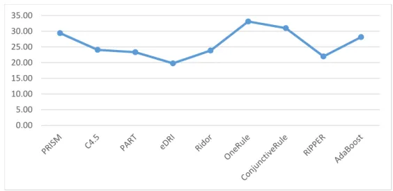
Figure 4.1 Error rate generated by the considered classification algorithm against the 20 datasets……….78
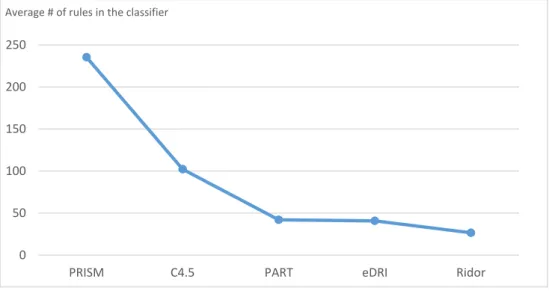
Figure 4.2 Average # of rules generated by the selected rule based classification algorithms against the 20 datasets………....…………..81
Figure 4.3 Average time in ms generated by the considered classification algorithms against the 20 datasets ... 82
Figure 4.4 error rate generated by CBA and the considered classification algorithms against the 8 least # of attributes ... 84
Figure 5.1. Example of an early phishing attack (Blogonlymyemail.com) ... 90
Figure 5.2. Phishing life cycle (Abdelhamid et al., 2014) ... 92
Figure 5.3. Phishing as a classification process ... 94
Figure 5.4 The One error rate (%) of the considered algorithms on the phishing dataset ... 117
Figure 5.5. The One error rate (%) of the considered algorithms on the reduced nine features phishing set chosen by CFS filtering ... 119
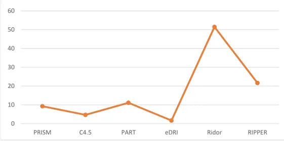
Figure 5.6. Number of rules generated by the rule-based algorithms from the phishing data ... 120
Figure 5.7. Number of rules generated by the rule-based algorithms from the nine features
phishing data ... 120
Figure 5.8 Time in ms taken to build the models by the considered algorithms from the security data. ... 122
Figure 5.9 Time in ms taken to build the models by the considered algorithms from the reduced nine variables security data. ... 122
List of Tables Table 2.1 A multi-label dataset……….…18
Table 2.1B Multi class dataset transformed from table 2.1A……….…...19
Table 2.2 Sample dataset (Grzymala-Busse, 2010)……….…..37
Table 3.1A Training dataset sample …….…..……….….53
Table 3.1B Transformation of Table 3.1A ……….…...53
Table 3.2: Items occurrences after initial scan by eDRI………...……….…54
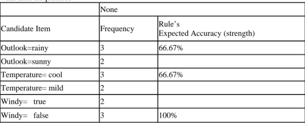
Table 3.3: Sample training dataset from (Witten and Frank, 2005)……….…...60
Table 3.4: Candidate items linked with class NO………...……..61
Table 3.5: Data samples associated with item “Outlook=sunny”……..……… 62
Table 3.6: Candidate items linked with item “Outlook=sunny” Then NO in the training dataset with their frequencies……….….……...62
Table 3.7: Candidate items linked with class YES……….…...63
Table 3.8: Training data samples linked with “Humidity=normal”………...…..63
Table 3.9: Candidate items linked with item “Outlook=sunny” Then NO in the training dataset with their frequencies………...64
Table 4.1: Confusion matrix for ASD diagnosis problem………..…73
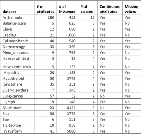
Table 4.2: The UCI datasets characteristics……… 75
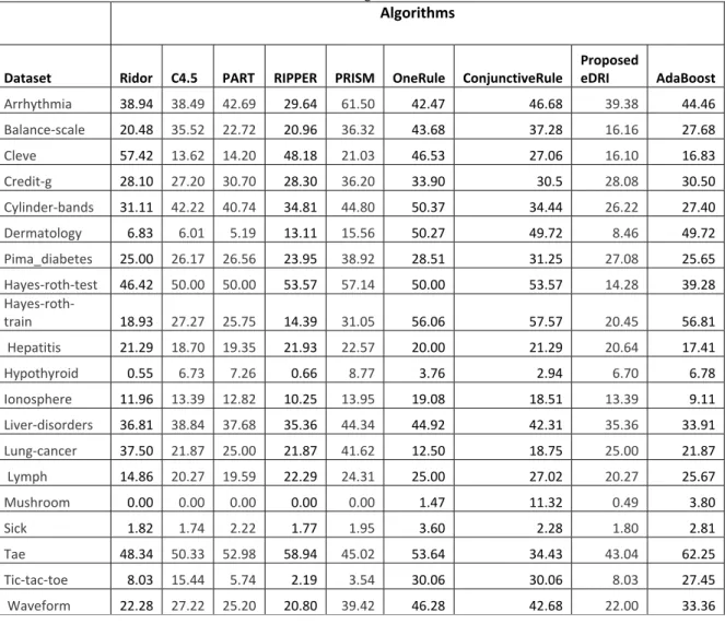
Table 4.3: The considered algorithms error rate for the UCI datasets……… 79
Table 4.4: The considered algorithms time in ms to generate the rules from the 20 UCI datasets……… 83
Table. 4.5 Runtime in ms generated by CBA and the considered classification algorithms against the 8 least # of attributes datasets……….……..85
Table 4.6: # of scanned data samples during building the classifier by PRISM and eDRI on the UCI datasets……….. 86
Table 5.1: Phishing Features per category (Aburrous, et al., 2008)………..111
Table 5.2 Common recent anti-phishing methods based on ML………...113
Table 5.3: Sample of twelve websites from the dataset and for eight features……….115
Table 5.4: Phishing features derived by Correlation Features Set filtering method along with their information gain scores……….118
List of Algorithms
Algorithm 2.1 PRISM Pseudo code……….………..…..26 Algorithm 2.2 Incremental Reduced Error Pruning procedure………. .. 32 Algorithm 2.3 Growing Rule Function used in REP, IREP and RIPPER algorithms…...… . 33 Algorithm 2.4 Single global Covering function of LERs and its variations (Pawlak, 1991)..36 Algorithm 2.5 CN2 original rule generation function (Clark and Niblett,1989)…...……..38 Algorithm 2.6 FOIL algorithm (Quinlan, 1990)………...…. ... 40 Algorithm 2.7 One Rule Pseudo code ………..………...42 Algorithm 2.8 Ridor algorithm pseudo code (Gaines and Compton, 1995)……..…………. 42 Algorithm 3.1 eDRI Pseudococode ………..……… ... 51 Algorithm 3.2 eDRI Learning Phase……….………..……… .... 56 Algorithm 3.3 Predicting test cases procedure of eDRI………..……… .... 57 List of Acronyms AC Associative Classification AOL America Online
ANN Artificial Neural Network
APWG Anti-Phishing Work
Group ARL Average Rule Length
CANTINA Carnegie Mellon Anti-phishing and Network Analysis
Tool CBA Classification Based on Associations
CFS Correlation Feature Set DM Data mining
DROP5 Decremental Reduction Optimization Procedure 5
eDRI Enhanced Dynamic Rule Induction
ENN Edited Nearest Neighbor FFNN Feed Forward NN
FOIL First Order Inductive Learner
IG Information Gain
IREP Incremental Reduced Error Pruning
LERS Learning from Examples Based on Rough Sets
MaT Monitoring and Takedown
MDL Minimum Description Length NN Neural Networks
OPUS Optimized Pruning for Unordered Search
PILFER Phishing Identification by Learning on Features of Email Received
PMCRI Parallel Modular Classification Rule Induction
REP Reduced Error Pruning
RIONA Rule Induction with Optimal Neighbourhood Algorithm
RIDOR Ripple Down Rule learner
SLIPPER Simple Learner with Iterative Pruning to Produce Error Reduction
SSL Secure Socket Layer
TF-IDF Term Frequency Inverse Document Frequency
UCI University of California Irvine
VV Variable Value
RIPPER Repeated Incremental Pruning to Produce Error Reduction
SVM Support Vector Machine
WARL Weighted Average Rule Length
WEKA Waikato Environment for Knowledge Analysis
WOT Web of Trust
Chapter One
Introduction
1.1 Introduction
Data mining (DM), which is based on computing and mathematical sciences, is a common intelligence tool currently used by managers to perform key business decisions (Abdelhamid & Thabtah, 2014). Traditionally, data analysts used to spend a long time gathering data from multiple sources and little time was spent on the analysis due to limited computing resources. However, since the rapid development of computer networks and the hardware industry, analysts are spending more time on examining data, seeking useful concealed information. In fact, after the recent development of cloud computing, data collection, noise removal, data size, and data location are no longer obstacles. Data analysis, or DM, is concerned about finding hidden patterns from datasets that are useful for users, particularly managers, to conduct suitable planning (Thabtah & Hamoud, 2014).
One of the known DM tasks, which involves forecasting class labels in previously unseen data based on models (classifiers) learnt from training datasets, is classification (Hall, et al, 2009). Generally, classification is performed in two steps: constructing a model, which is often named the classifier, from a training dataset, and utilising the classifier to predict the value of the class of test data accurately. This type of learning is called supervised learning because while building of the classifier the learning is guided toward the class label. Common applications for classification are medical diagnoses, web security, and stock market analysis (Rameshkumar, et al, 2013; Mohammad, et al, 2015; Dash & Dash, 2016), etc.
One of the least studied approaches in classification is that which is based on separate and conquer learning (Pagallo & Haussler, 1990). This learning approach normally splits the training dataset into subsets based on classes and discovers the rules for each class
through relationships between the input dataset’s variables and class values. Once the complete set of rules is discovered, a classifier is formed by integrating the rules.
This thesis focuses on rule-based classification models, particularly Covering approaches in DM. It proposes new dynamic Covering classification techniques that generate predictive models. These models contain knowledge represented as “if-then” rules, therefore they can be easily understood and maintained by decision makers. This chapter discusses the research problems under investigation, as well as the major contributions achieved. Lastly, we outline the structure of this PhD report.
1.2 Motivation
Supervised learning is one of the common learning approaches in machine learning (ML) and DM. In supervised learning, a model is normally constructed from a labelled set of examples called the training dataset. A typical training dataset consists of a set of variables (features) and a special variable called the class. For example, in medical diagnoses the class is the type of illness, and for credit card scoring the class is whether an applicant is granted credit or not. The primary purpose of the classifier is to accurately predict the class of an unseen dataset called the test dataset. There have been many different classification approaches proposed by researchers in the last few decades,
including Decision Trees, Neural Network (NN), Support Vector Machine (SVM), Associative Classification (AC), and Covering among others (Quinlan, 1979; Mohammad, et al, 2013; Cortes & Vapnik, 1995; Thabtah, et al, 2004; Holt, 1993). The latter two approaches, AC and Covering, extract classifiers that consist of rules, which explain their wide applicability. However, in practise there are differences between AC and Covering, in particular in the way rules are induced and pruned. This thesis falls under the umbrella of Covering rule-based classification research.
There are a number of distinguishing features for Covering approaches in classification. The most dominant being that they are easy to understand models. Unlike models devised by traditional classification models such as NN, decision trees, or SVMs which normally require a domain expert to interpret them. The simplicity of Covering based models can be attributed to the straightforward rule format used, which novice users can easily interpret and utilise in decision making (Abdelhamid, 2015). Another
noticeable feature of rule-based models is that users can easily maintain the classifier by adding, removing, or even amending rules when needed (Witten & Frank, 2005). This feature is hardly accomplished in other predictive models such as Decision Trees. Indeed, in decision trees the entire tree (classifier) must be reshaped if one tries to add a branch or partial tree to the existing tree, which is a complex process. Lastly, in Covering approaches, rules are ranked in a way that enables end users differentiate between highly effectives rules (mostly ranked at the top of the models) and less effective rules. This ranking is vital in choosing the rule or the set of rules that are able to predict the test cases, and therefore ranking influences the number of test data misclassifications.
The methodology in most existing Covering classification algorithms requires splitting the training dataset into a number of subsets based on class labels before the training phase begins. This approach was criticised by scholars in ML and DM because it builds local classifiers that belong to a subset of the training dataset rather than a complete training dataset (Abdelhamid & Thabtah, 2014). This criticism is attributed to the fact that rules are generated per class rather than from the entire classes at once, and in some cases a variable value belonging to multiple classes is considered only with the most frequent class during the training phase. This can also cause the generation of only single rules (one class per rule).
Another obvious problem associated with Covering techniques is the large numbers of rules induced, which normally leads to large classifiers (Witten & Frank, 2005). This problem appears because of the way the algorithm induces the rules; it keeps adding items to the rule’s body until it covers only positive training data examples. In other words, the Covering algorithm typically produces many rules, each covering only a few examples of positive data, rather than rules covering large numbers of positive and negative data samples. The outcome of the aforementioned excessive learning is a classifier with several specific low data coverage rules that may overfit the training dataset. This may limit the use of this learning approach to domains that require a concise set of rules for decision making. Often managers in application domains such as medical diagnosis or credit card scoring prefer a summarised set of rules that they can manage instead of a high maintenance set of rules. There should be compromise between the number of rules and the predictive accuracy.
A more crucial issue that is worth investigating in Covering classification is the way rules are induced. When a rule is discovered, the algorithms directly delete its corresponding positive training data. The Covering algorithm then scans the adjusted training data to discover the next rule, produce it, remove its linked data, and then scan again the newly adjusted training data and so on (Abdelhamid & Thabtah, 2014). This repetitive process, especially the multiple data scans, consumes large computing resources and should be dynamically implemented.
This thesis investigates shortcomings associated with Covering algorithms in data mining. Specifically, we look at research issues including but not limited to the following:
1) Minimising computing resources, especially the number of passes over data examples, by proposing a dynamic learning technique.
2) Reducing the search space for both items and rules to make the training phase more efficient.
3) Generating smaller predictive models without hindering predictive power so end users can manage the classifiers in a straightforward manner.
4) Derive good quality rules, not necessarily with 100% accuracy, to reduce over-fitting and increase data coverage per rule.
5) Generating web security models based on Covering approach to serve as an anti-phishing rules set. This is since novice users usually prefer easy to understand rule to make them better understand phishing activities and features.
6) Identifying small, effective, phishing features.
This thesis involves only binary and multi-class classification problems since they are more common in classification applications. These problems produce datasets with examples, which are linked with one class. In other word, each instance in the training dataset is connected with one class value. The multi-label classification case is out of the scope of this thesis since they have different data format and requires special transformation. The scope is limited to the Covering approach in data mining, so other approaches related to generating rules such as Associative Classification are not explored. Associative Classification methods are based on association rule so they require the
complete rule sets to be derived using unsupervised learning search before building the classifiers.
1.3 Covering Induction Process and Related Definitions
In Covering Classification approach, knowledge is discovered readily as the algorithm typically discovers rules per class label. For each class, i.e. C1, the algorithm makes an empty rule (if empty then C1) and looks for the best variable value (VV), such as Max VVi, which leads to the largest gain according to a certain metric, or accuracy, with C1. The rule’s accuracy can be achieved by dividing the combined frequency of VVi and the class, C1, by the number of data examples that belong to VVi in the training dataset.
The algorithm merges the VVi with the largest accuracy with the rule’s antecedent (left hand side), and proceeds to search for the next VVi+1 in the training dataset with which to append. The algorithm terminates building the rule when no more VVi with acceptable accuracy can be found, and at that point the rule is generated and all of its positive examples that belong to C1 are discarded. The algorithm continues discovering the rules from the remaining data examples that belong to class C1 until that set becomes empty, or no VVi when integrated with C1 has an acceptable accuracy. When this occurs, the algorithm moves on to the next class data set and repeats the aforementioned steps until the complete rules set is derived.
The problem can be formally defined as follows: Given a training dataset T, which has
x distinct columns (variables) V1, V2, … ,Vn, one of which is the class, i.e. class. The size
of T is |T|. A variable in T may be nominal, which means it takes a value from a predefined set of values, or continuous. Nominal attribute values are mapped to a set of positive integers whereas continuous attributes are pre-processed by discretising their values using any discretisation method.
The aim is to construct a classifier from T, e.g. Classfiier :V class, which forecasts the
class of a previously unseen dataset.
The classification method investigated employs a user threshold called freq. This threshold serves as a fine line to distinguish strong rule items <item, class> from weak ones based on their computed occurrences in T. Any rule item whose frequency bigger
than the freq is called a strong rule item, otherwise being referred to as a weak rule item. Below are the main concepts used throughout the thesis and their definitions.
Definition 1: A variable plus its denoted values name (Vi, vi) is known as item
Definition 2: A training example in T is a row consisting of variable values (Vj1, vj1), …,
(Vjv, vjv), plus a class denoted by classj.
Definition 3: A rule item r has the format |body, c|, where body is a set of disjointed items
and c is a class value.
Definition 4: The frequency threshold (freq) is a predefined threshold given by the end
user.
Definition 5: The body frequency |body_Freq| of a rule item r in T is the number of
training examples in T that matches r’s body.
Definition 6: The frequency of a rule item r in T (ruleitem_freq) is the number of training
examples in T that matches r.
Definition 7: A rule item r passes the freq threshold if, r’s |body_Freq|/ |T| ≥ freq. Such
a rule item is said to be a strong rule item.
Definition 8: The rule strength |rule_strength| is a predefined threshold given by the end
user.
Definition 9: A rule r has a strength which is defined as |ruleitem_freq|/ |body_Freq|. Definition 10: A rule r can be generated when r’s |strength|>= |rule_srtength|.
Definition 11: A rule takes the form: r: body class , where body is a set of disjoint
variable values and the consequent is a class value. The format of the rule is:
1 2
1 v ... v class
v n
1.4 Thesis Research Issues
Different issues related to rule based classification approaches, particularly Covering classification, are discussed in this research. These are:
Developing a dynamic rule discovery process.
Improving the performance of Covering techniques.
o The reduction of the search space of items during training phase.
o Generating a concise set of rules by removing redundant rules in the
classifier.
o Minimising over-fitting the training dataset.
o Improving training time required to construct models.
Domain Specific Issues
Covering classifiers as an anti-phishing tool.
Determining the most effective features related to phishing.
1.4.1 Generic Issues
GI-Issue 1: The Methodology to Discover the Rules
In most rule-based classification the process of rule discovery is accomplished in a separate phase after the algorithm goes over the training dataset to record item and class occurrences. For each available class, these algorithms add the best item to the class according to a certain measure of the rule’s body. When the rule reaches the desirable accuracy, then it gets derived and these algorithms discard all classified training data examples that belong to the rule. The algorithm then proceeds to discover other potential rules for the class at hand from remaining data examples by reviewing the complete dataset again, wasting runtime and memory. This step is necessary, however, since the frequency computed earlier for the items and the class labels for some potential rules have changed. This process not only is resource demanding, but can also cause the algorithm to crash when the data is highly dimensional. A simple experiment using the PRISM Covering algorithm implemented in WEKA ML tool against a “Segment Challenge” dataset downloaded from the University of Irvine data repository was conducted to record how many data examples this algorithm must go over to learn the rules (Cendrowska, 1987; Hall, et al., 2009; Licham, 2013). The “Segment Challenge” dataset consisted of twenty variables and 1500 examples. It turns out that this methodology must scan
7,147,542 data examples to find the rules. This number can be of higher magnitude if datasets with larger dimensionalities are used, which is a burden in big data domains.
Contribution
There should be a mechanism embedded in the training phase which ensures that the rank and frequency of potential rules are amended in a dynamic manner without any repetitive training data scans. This will make the process of rule induction efficient, not static every time a rule is derived. Therefore, whenever a rule is inserted into the classifier all remaining potential rule <item,class> occurrences should be updated extemporaneously based on data removal. We developed a new dynamic rule learning that substantially reduces the number of examples scanned. Our method, which we called Enhanced Dynamic Rule Induction (eDRI) Qabajeh, et al, (2014) is presented in Chapter three.
Experimentations using different classification datasets that belong to applications beyond medicine, credit card scoring, finance, agriculture, politics, and others from UCI data repository (Lichman, 2013) have been conducted to evaluate the proposed eDRI. Chapters four and five give further detail on the compared algorithms, experiment settings, evaluation measures, and data characteristics. The results show that eDRI outperforms other classic ML algorithms as well as rule-based algorithms in regard to the considered evaluation measures. Moreover, models produced by eDRI not only have good predictive power, but they are also efficient during data processing and contain small effective rules for decision making. These rules have low to no redundancy since they do not overlap in the training examples and normally require a lower number of data scans to be found that the compared Covering algorithms.
GI-Issue 2: Enhancing the Performance of the Classification Models
(Classifiers)
We investigated different problems in rule-based classification related primarily to the process of rule discovery and classifier content. These issues are:
Reducing the search space for items
Improving test data prediction by using multiple rules based on weights A. Cutting down the items search space during the training phase
As mentioned before, in typical rule-based classifiers such as Covering the methodology to find the rule necessitates that after generating each rule a full scan is conducted on the remaining data examples. This is necessary to record item frequencies after data removal; hence, the search space of items is massive and consequently consumes large computing resources. In fact, the number of items that can participate in rule induction should be minimised since many of these items have no statistical significance and removing them will improve the process of creating rules. Thus, there is a need for a mechanism that discriminates between items to reduce the numbers of items in the search space during the training phase.
Contribution
The rule discovery process proposed in the enhanced Dynamic Rule Induction algorithm (eDRI) minimised the number of items that can be offered to the rules. We have introduced a frequency threshold (freq, see Definition 6) that discriminates among items based on their occurrence with the item and class in the training dataset. The freq threshold serves as an indicator that distinguishes weak items from strong items. Any item plus class frequency must pass the freq threshold so it can be considered by the rules. This has reduced the search space for items during rule building by discarding weak items early on and in a dynamic manner. In fact, strong items can become weak whenever a rule is derived if they appeared in the discarded rule’s data. Experimental studies in Qabajeh et al, (2015) showed an improvement in use of computing resources, especially run time reduction and number of passes required for building the classifier. These results are documented in Chapter 4.
B. Reducing the number of rules for better controllability
One of the drawbacks associated with Covering algorithms is that despite being simple classifiers, the number of rules they produce is large. This can be attributed to the way the algorithm discovers rules in that each correlation between class and variable is
investigated and which leads to the production of several specific rules (covering very limited data examples). Most Covering algorithms, like PRISM and its successors, keep appending variables into the rules body until the rule achieves a zero error rate. This can result in just covering one or two training data examples, which limits generalising rule performance across wider data applications. To overcome this issue, we investigated this problem and proposed a rule pruning procedure to cut down the number of potential rules and reduce the classifier size. It should be noted that search induction learning algorithms such as PART, IREP and RIPPER use extensive such as backward and minimum description length principle pruning to cut down the size of the classifiers (Frank & Witten, 1998). However, these algorithms originally employ a divide and conquer approach to learning trees that then are converted into classification rules. Thus, it is impractical and incorrect to consider them Covering approaches despite generating rules.
Contribution
We have developed a pruning method that ensures each potential rule has a true rank during the process of rule generation. When a rule is constructed, and its data examples are discarded, we immediately adjust the potential rule ranks which help us to determine weak rules early on and remove them. The resulting analysis against a large data collection from the UCI repository showed moderate size models being consistently generated by our dynamic technique when compared with those generated from decision trees and other Covering algorithms. Interestingly, the models produced by eDRI had a lower number of rules yet the predictive performance was sustained for the majority of datasets. Furthermore, in phishing detection, eDRI was able to construct small set of useful anti-phishing rules that contained new and interesting information for security experts and online users. Lastly, when the phishing data was processed, the accuracy of our incremental model was only slightly affected, which shows constant predictive performance of eDRI on different domains data. All the aforementioned results are elaborated in details in Chapters 4 and 5.
C. Avoiding Over-fitting and Under-fitting
One of the important issue in supervised learning predictive models is over-fitting the training dataset. This problem is obvious in Covering approach when the learning algorithm excessively trains against the input dataset particularly when the algorithm allows the generation of only perfect rules, which is true case with PRISM. These rules usually are associated with maximum accuracy against the training dataset, yet they are not general rules that can be widely applied on an unseen dataset. Therefore, the predictive performance of the rules when they are applied on a test dataset is questionable. Another obvious example is the REP algorithm that generates a complete rule set and then invokes an evaluation step to cut down redundant rules (Fürnkranz & Widmer, 1994). There should be a mechanism for learning to be stopped so that training datasets will not be overfitted. This mechanism guarantees realistic rules in the final classifier that are linked with insufficient data representation being discarded early during the training phase.
Contribution
We posit that generating high quality rules, not necessarily perfect ones but rather those with larger classified training examples, is advantageous. This can be accomplished using user statistical measure such as rule strength (see definition 9). The rule strength separates acceptable from unacceptable rules based on both data coverage and items’ frequency within the class label. This is important because applications such as phishing classification necessitates small yet highly correlated rules in the classifiers. Rule strength serves as a point at which we stop adding items into the rule’s body and therefore reduce over-fitting the training data by allowing for a slight error per rule while maintaining larger data coverage. Moreover, rule frequency dynamically during the training phase contributes to reducing over-fitting. This is since items within potential rules that fail to accomplish the frequency threshold will be discarded, and therefore these rules will not be considered during the training phase and consequently further shrinks the search space.
1.4.2 Domain Specific Issues
Phishing is one of the most serious online frauds, costing different stakeholders including banks, online users, governments, and other organisations severe financial damages. This fraud often entails designing and implementing a replica website that maintains visual similarity to that of an existing trusted organisation (Aburrous, et al, 2010). The aim of phishing is to unlawfully obtain user login data in order to access their financial information (Mohammad, et al, 2015). One promising research direction to minimise the risks of phishing is using predictive ML and DM algorithms. Despite promising results with reference to classification accuracy of the aforementioned approaches, the models they produce are usually complicated in a way that novice users might find difficult to interpret and use them for making decisions. Moreover, adding to or amending the model requires careful implementation and is often a complex process that end users might be unable to perform (Abdelhamid, et al, 2014).
Contribution
A model with straightforward knowledge represented in simple rules is obviously advantageous for end users. Not only the model could be used to detect phishing activities, but it could also serve as a decision making tool in which the user can readily understand the relationship between phishing features and the website’s class, i.e. phishy or legitimate. There has been recent research on the use of rule-based classifiers utilising associative classification reported in Abdelhamid (2015) and Abdelhamid, et al (2014). However, these approaches suffer from noticeable drawbacks, which are not limited to just the size of the classifiers derived but also the inherited problems from association rules such rule redundancy. A Covering approach that enhances the process of rule discovery and classifier building as discussed in Section 1.4.1 and removes data overlapping can be an effective anti-phishing tool. To date, there is very limited work on anti-phishing using covering classification.
A case study, Chapter 5, that investigates phishing as a classification problem is reported. This chapter contains critical analysis of phishing approaches, from traditional to education and intelligent ones, with their associated benefits, disadvantages and ways forward in combatting phishing. More importantly, a comprehensive experimental study on real phishing websites is reported. eDRI’s performance as a phishing detection
technique is compared against the performance of other ML techniques to reveal the strengths and weaknesses of eDRI.
1.5 Thesis Structure
This thesis consists of five chapters including the present one. Chapter two critically analyses Covering techniques in data mining, separate and conquer, divide and conquer, and their mutually common algorithms. We have included induction learning approaches as well. Chapter three is devoted to the proposed Covering algorithm (eDRI) for constructing rule-based predictive models. In chapter three, we present the dynamic process mechanism, pruning procedure, class forecasting method and a detailed example that explains eDRI insight. Chapter four contains the implementation of our newly enhanced dynamic method during the training phase. We also present the evaluation measures used and phase details of our algorithm alongside a complete example. In addition, the results on the UCI datasets and their analysis are discussed in chapter four. These are not only limited to large variations of UCI datasets, large selection of rule and non-rule based ML algorithms, and evaluation measure results analysis. Real data experimentations related to phishing and using a number of ML techniques have been conducted in chapter five. This section also reviews and critically analyses the phishing problem and traditional solutions based on legal, educational, and intelligent anti-phishing tools. A large experimental analysis is then conducted to evaluate the benefits and disadvantages of the proposed algorithm. Lastly, chapter six concludes the thesis by responding to the research issues raised in chapter one and highlights the main contributions of this thesis, further pinpointing possible future research paths.
Chapter Two
Covering and Induction Approaches in
Classification
2.1
Introduction
One of the primary tasks in ML is predictive classification (Diebold and Mariano, 1995; Abdelhamid, et al., 2016). In classification, a predictive model called the categoriser/classifier is typically constructed from a training dataset. This model is then applied to test data in order to predict the class as accurately as possible. Effectiveness of the model is measured mainly on its performance in predicting test cases (Abdelhamid and Thabtah, 2014). The less number of misclassifications the model scores on test data cases the higher predictive power the model possesses and therefore its performance can be generalised.
There are two forms of classification problems; single label and multi-label (Fürnkranz, et al., 2008). The former can also be classified into two types: binary and multi-class classification. In binary classification, training data can only be linked to a single class value from two possible values in the training dataset, while in multi-class classification each training instance is linked with one class value from two or more possible values. On the other hand, multi-label classification problems necessitate that each training instance has multiple class values, and thus this type of data requires careful transformation (Taiwiah and Sheng, 2013). This is since each instance must be repeated with each class label. More details on the different classification problem types are given in Section 2.2.
Different intelligent learning methodologies based on DM and ML have been developed and disseminated to deal with the classification problem. Among these we have support vector machine (SVM), neural network (NN), associative classification
(AC), boosting, regression trees, probabilistic, decision trees, induction learning, and Covering among others (Joachims, 1999; Mohammad, et al, 2012; Liu, et al, 1998; Abdelhamid, 2015; Freund & Schapire, 1997; Breiman, et al, 1984; Duda, 1973; Quinlan, 2002; Cohen, 1995; Bramer, 2002). The majority of the learning approaches solve classification by decomposing the problem into two phases discussed berfore
Learning Phase: This phase involves learning a model from the training dataset.
Prediction Phase: Using the learned model to predict the class label value in a test dataset.
In this thesis we deal with Covering classification, yet in Section 2.3 other common induction ML approaches that are suitable to solve the classification problem are still discussed.
As mentioned in Chapter One, Covering classification is one of the most important learning approaches that generate predictive models with Then” rules. These “If-Then” rules can be utilised as a knowledge base by end-users for decision making (Qabajeh, et al., 2015). A typical Covering algorithm learns rules one by one and for each available class in the training dataset. The algorithm initially creates an empty rule for a specific class [If empty, then Class 1]. Then using certain mathematical metrics such as accuracy, foil gain, etc., append one item to the empty rule body (left hand side)(Cendrowska, 1987; Quinlan, 1990). The algorithm keeps appending items until the rule metric cannot be further enhanced, at which point the rule is inserted into the classifier. In the same manner, the algorithm continues deriving the rules for the classes until a stopping condition is met.
Three noticeable characteristics exist of a Covering approach in solving classification problems (Clark & Boswell, 1991; Domingos, 1996a; Grzymala-Busse, 2010; Abdelhamid & Thabtah, 2014)
The learned model contains simple yet highly influential rules for decision making that end-users can easily comprehend and manage.
Adding new knowledge (rules) can be done in a straightforward manner.
This chapter defines classification problems, followed by discussing classic induction learning approaches. More importantly, the focus will be on Covering classification methods as well as other common rule-based classifiers. The chapter structure is as follows: the classification problem and its main steps are discussed in Section 2.2; classic learning strategies dealing with predictive tasks such as classification are briefly discussed in Section 2.3, while section 2.4 critically analyses Covering classification approaches along with other common rule-based classifiers in DM and ML. Moreover, we also introduce non-rule classification methods such as Boosting, probabilistic, SVM, AC and NN in section 2.5. Finally, conclusions are drawn in section 2.6.
2.2
The Classification Problem and Its Variations
In Chapter One, we have discussed the main terminologies related to the classification problem, specifically those connected with the Covering approach. In this section, we define single label classification problems (both binary and multi-class) in the ML context. Figure 2.1 depicts the essential steps that any learning algorithm goes through in order to construct models and apply them to predicting test cases. Input will consist of a set of labelled variables, including the class, called the training dataset. A learning algorithm then processes the training dataset to derive the classifier. This classifier is then applied to a test dataset to measure its prediction power (see Figure 2.1).
Multi-label and multi-output classifications are variants of the classification problem where multiple target labels must be assigned to each test case (Veloso , et al, 2007). Multi-label classification should not be confused with multi-class classification, which is the problem of categorising instances into one of more than two classes. Formally, multi-label learning can be phrased as the problem of finding a model that maps inputs (x) to binary vectors (y), rather than scalar outputs as in the ordinary classification problem (Tsoumakas, et al, 2010).
In binary classification and according to Bradley, et al (1998), given an input dataset taking the format of (Xi, Ci) we can assign the given vector xin into one of two disjoint sets A or C in a dimensional variable space where n. Xin is the ith data instance and Ci {1, ….., K) is the ith class. The ultimate goal is to derive a function, F, that maximises the chance that F(x) = Ci for an unseen data instance. The classification problem can basically be transformed into a two class problem in which the class ci can be either 0 or 1. This simple format of the problem is called binary classification. Binary classification function, F(x), has the following format:
1 0 C x A x
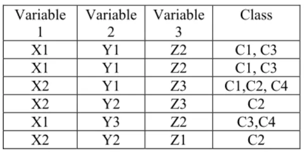
Multiclass classification deals with predictive problems that involve more than two values for the class label.This is because the training dataset in multi-label classification, such as an image or a science, contains instances where each may be associated with multiple labels rather than a single class as in multi-class or binary classification (Tsoumakas, et al, 2010). Tables 2.1a-2.1b depict multi-label and multi-class datasets, respectively. Table 2.1b is the transformation of Table 2.1a from multi to single label classification.
Often multi-class and multi-label datasets require data transformation, so strategies that transform their datasets into binary classification are essential. Two of the common data conversion strategies from multi-class and multi-label into a binary classification are one-versus-one and one-versus-all (Fürnkranz, et al, 2008). The latter essentially learns single classifiers for each class label. While learning the classifier for a class C, all training instances that belong to C are considered positive instances and the remaining are negative instances. Thus, when a test case is about to be predicted, a score based on
the required single classifiers is calculated to come up with the class decision (Thabtah et al, 2006). One shortcoming associated with the one-versus-all approach, however, is when the training dataset is imbalanced because it potentially creates a computed score that can be arisen with biased to the majority class. The other data conversion strategy, the one-versus-one approach, necessitates producing N (N− 1) / 2 binary models for the
N multi-class problem (dataset)(Thabtah, et al, 2006). When test data is about to be predicted, a voting mechanism is employed in which all N (N− 1) / 2 are utilised and the
class with the largest correct predictions is assigned by the multiple binary models. According to Tsoumakas, et al, (2010), for multi-label classification problems two data processing methods are also used; problem transformation and algorithm adaptation. The problem transformation consists of converting of the available multi-label dataset into binary classification sets in that each set can then be dealt with using any binary classification methods. In other words, the problem transformation strategy can be seen as a pre-processing phase which ensures that each training instance in the original multi-label dataset is transformed into multiple single multi-label instances. On the other hand,
Table 2.1A multi-label dataset Variable
1 Variable 2 Variable 3 Class
X1 Y1 Z2 C1, C3 X1 Y1 Z2 C1, C3 X2 Y1 Z3 C1,C2, C4 X2 Y2 Z3 C2 X1 Y3 Z2 C3,C4 X2 Y2 Z1 C2
Table 2.1B multi-class dataset transformed from Table 2.1A Variable
1 Variable 2 Variable 3 Class
X1 Y1 Z2 C1 X1 Y1 Z2 C3 X1 Y1 Z2 C1 X1 Y1 Z2 C3 X2 Y1 Z3 C1 X2 Y1 Z3 C2 X2 Y1 Z3 C4 X2 Y2 Z3 C2 X1 Y3 Z2 C3 X1 Y3 Z2 C4 X2 Y2 Z1 C2
algorithm adaptation strategy employs a specific algorithm to learn multi-label models directly from the multi-label classification datasets without the use of data pre-processing phase. This approach to learning from multi-label problems is domain specific, and requires different learning strategies to acknowledge the fact that an instance has multiple class labels and the prediction involves assigning multiple labels to the test data.
This thesis focuses only on binary and multi-class classification, and leaves multi-label classification out of scope of this study since this requires effort for additional PhD.
2.3 Learning Strategies in Classification
2.3.1 Divide and Conquer
This classification approach splits data into subsets, which are further divided into smaller divisions until the algorithm believes that the subsets are adequately homogenous or the stopping criterion has been satisfied (Quinlan, 1979). To illustrate this, imagine a root node being the entire dataset. Subsequently, the algorithm specifies a variable in the dataset to start the first split. In an ideal situation the algorithm starts with the feature that maximises discrimination among the outcome classes in the dataset. Decision tree algorithms which apply divide and conquer use Gini index or Information Gain metrics to select the variable that can be the root node (Zaremotlagh, S., & Hezarkhani, 2017; Gini, 1999; Quinlan, 1986). The cases are next grouped into classes based on the splitting of the variable. This process is repeated and the algorithm continues to separate (divide) and group cases while excluding heterogeneous data cases (conquer).
Decision tree algorithms are common divide and conquer methods that classify cases based on their attributes’ values. Nodes represent variables to be classified, and branches represent the values that variables take (see Figure 2.2). Cases are classified beginning at the root node. Figure 2.2 represents a decision tree for a tax evasion classification problem (Tan, et al, 2005). Based on a number of attributes (tax refund and taxable income along with demographic information and marital status), the user wants to predict whether citizens cheated on their tax forms.
Note that the attribute that best classifies the cases is represented by the root node feature. In this example, marital status seems to be the best one. Married people did not cheat on their taxes as the first node of the tree indicates. The process of classification
based on best features continues until a parsimonious representation is obtained. Decision trees are useful given their representations for classification problems, which constitute a large portion of everyday applications. The detailed process of how to construct decision trees from training dataset and common methods used are given below.
Imagine that you are a university administrator working for a public university. Your role is to decide whether new programmes should be approved for enrolment in the next academic year. Upon your return from holiday, your work station is full of requests from various colleges. Realising that you do not possess sufficient time, you decide to construct a decision tree to help make the decision of categorising the requests into three groups: Success, Revision and Failure. To construct the decision tree, you explore factors associated with the 20 most successful and 20 worst programmes at the university during the past 25 years. You realise that there is a strong correlation between the programmes’ budget, size, and college affiliation of programme with the probability of its success or failure. Beginning with the entire dataset, the root node, we can select programme budget as the first feature by which to split programmes. Programmes can be classified as having a cost of more than $1 million or less. Second, among the programmes with a cost of less than $1 million, we can classify them based on their college affiliation. We could further split the programmes, yet over-fitting a tree is non-advisable. Over-fitting occurs when someone is trying to over learn by building larger trees in order to maximise the predictive performance of the model (tree) on the training dataset rather than on the test dataset (Hall, et al, 2009). You could therefore decide that programmes meeting a cost of less than $1 million dollars within a technical college affiliation are more successful, and thus approve them.
Despite its applicability, the divide and conquer approach, it suffers from a number of limitations (Kothari & Dong, 2000; Leung, 2007; Grzymala-Busse, 2010). First, it tends to split the data based on variables with a large number of levels. Second, it is easy to over-fit or under-fit a model for classifying instances in a given dataset. Under-fitting the model occurs when someone stops building the tree early, and thus produces a model with limited performance (Witten & Frank, 2005; Jankowski & Jackowski, 2014). Third, the divide and conquer approach is problematic when it comes to modelling complex relationships since it relies on axis-parallel splits. Moreover, the output produced,
audiences. In this event, the user will not be able to manage the tree and therefore will not be able to use it for decision making. Finally, a key weakness of the divide-and-conquer approach is its sensitivity to the input data (Leung, 2007; Grzymala-Busse, 2010). A small change in the input may result in significant changes in the decision trees produced. Introducing new cases into the dataset may result in redrawing the whole tree altogether. Despite the easy constructing decision trees, they tend to be more complex compared to other classification approaches, i.e. separate-and-conquer (see section 2.3.2) (Fürnkranz, 1999; Brookhouse & Otero, 2016), which This learning approach produces an easier representation of results, thereby making them superior to divide-and-conquer, particularly in their final models understanding.
2.3.2 ID3 Decision Algorithm
Decision trees in classification spread out after the dissemination of the ID3 algorithm (Quinlan, 1979). A decision tree can be constructed based on the available features inside the training dataset, primarily using the equation for Information Gain (IG) (Equation 2.1). The tree is built using the ID3 algorithm by initially selecting the attribute with the highest computed IG among all available attributes in the training dataset as a root node. IG is computed using Entropy (Equation 2.2) which denotes how informative a feature is in splitting the training instances according to the target attribute values. After choosing the root node, the algorithm computes IG repeatedly for the remaining attributes, excluding the root node until the tree cannot be divided any further or all training instances for an attribute belong to one class (Quinlan, 1993).
IG (T, f) = Entropy (T) -
((|Tf| / | T |) * Entropy Tf)) (2.1)Where Entropy (T) =
Pclog2Pc (2.2)where
v
P
= Probability that T belongs to class l. Tf = Subset of T for which feature F has value faA tree constructed by ID3 can be transformed into a rules set in which a path in that tree links the root node to any leaf making a rule. Figure 2.2 displays a tree that contains four rules that were constructed based on three features and a target attribute (class).
2.3.3 Separate and Conquer
Separate-and-Conquer is a learning strategy famous within the rule-based classification (Pagallo & Haussler, 1990; Fürnkranz, 1999; Rijnbeek & Kors, 2010). The classification problem is characterised by a number of positive and negative cases of a specific concept, normally called the class, and a set number of attributes inside a training dataset. The separate-and-conquer algorithm discovers the class in the form of explicit rules, or knowledge, composed of tests derived from values of attributes in the training dataset. The resulting set of rules should be able to explain instances of the target class and discriminate other instances that do not belong to it. Many approaches have been developed to solve this problem including covering and induction learning (Stahl & Bramer, 2014; Pazzani & Kibler, 1992).
Covering approaches are popular within rule-based classification. Despite their limited numbers of algorithms, they still constitute a viable approach in classification problems (Abdelhamid & Thabtah, 2014). Covering approaches are present in many free tools developed by the ML community such as R and WEKA (R Development Team, 2008; Hall, et al., 2009). Covering approaches have a number of advantages over other
approaches of rule-based classification especially the simple to define outcome rules. However, before we delve into their strengths, we need to describe their basic strategy in classification problems.
Covering algorithms are similar in the logic they adapt when solving a classification problem. This family of rules learning share a common feature: a separate-and-conquer algorithm that searches for a rule that predicts part of the training set, while are isolated those, and then conquers the remaining cases learning new rules until no cases are left in the dataset. This approach guarantees that each case in the training set is covered by at least one rule (Grzymala-Busse, 2010). Pagallo & Haussler (1990) developed the term separate-and-conquer in reference to the common feature of those algorithms. Other authors have referred to this approach in different ways, “separate-and-conquer,” “Covering ,” or “greedy” just to name few.
Covering approaches are characterised by a strong representation bias compared to other approaches such as classification tree algorithms (Fürnkranz, 1999). A simple rule is required to perform the same task a complicated tree would achieve. The separate and conquer approach tries to maximize the purity of a leaf when it attempts to generate a rule. On the other hand, classification trees look for the average purity when splitting a node. However, the rules do not possess the redundancy problem of the association rules approach. The underlying logic behind separate-and-conquer is to generate a parsimonious set of rules capable of classifying new cases by distinct rules within a dataset (Pagallo & Haussler, 1990). Covering approaches are more sensitive to collision problems when an instance could be classified into more than one rule (Witten & Frank, 2005).
Covering approaches work either in a bottom-up or top-down fashion (Grzymala-Busse, 2010). The bottom-up strategy begins with a positive case by attempting to generalise the rule through the removal of conditions. The basic assumption here is that the rule must cover the largest group of positive cases and the fewest number of negative cases. While valuable, this strategy is tedious and does not perform well in noisy datasets (Stahl and Bramer, 2012). The top-down strategy resembles the classification tree model. It aspires to maximise the purity of the leaf on a branch of a tree. Computationally, this strategy consumes equivalent time to that of the classification tree approach (Witten &
Frank, 2005). Hereunder are the main advantages and disadvantages associated with traditional Covering approaches based on the comprehensive review we have conducted:
Advantages
1) The simplicity of rules generation in which only one metric is computed to decide rule significance (Franczak, 2002).
2) The classifier contains easy rules which can empower decision makers, particularly in domain applications that necessitate quick and easy interpretations (Abdelhamid, et al, 2014; Abdelhamid and Thabtah, 2014)
3) Straightforward implementation, especially with available computing resources (Stahl and Bramer, 2014).
4) The predictive power of its classifier can be seen as acceptable when contrasted to other classic DM and ML approaches such as search methods, decision trees, NN, Boosting, Regression, AC, and many others (Bramer, 2002; Thabtah et al, 2007).
Disadvantages
1) Noisy datasets that contain incomplete attributes and missing values. This can be seen as a major challenge since no clear mechanism on handling noise is presented (Grzymala-Busse, 2010). Currently, adopted approaches from information theory are used to handle noise as in Bramer (2000), Stahl and Bramer (2014), and Cohen (1995).
2) No clear rule pruning methodology is present. This may lead to the discovery of large numbers of rules and therefore combinatorial explosion (Abdelhamid & Thabtah, 2014). There is a high demand on pruning methods to cut down the number of rules without hindering overall performance of the classifiers (Abdehamid, et al, 2014). One possible promising solution is pruning methods adopted by induction learning algorithms such as PART, IREP, and RIPPER because they use reduce-error pruning methods and therefore decrease the number of rules.
3) Conflicting rules during prediction. There is no clear mechanism on how to resolve conflicting rules (Grzymala-Busse, 2010). Currently the choice is random
and favours class labels with the largest frequency linked with the item rather than keep multiple class labels per item.
4) Breaking ties among item frequencies while building a rule. When two or more items having the same frequency, Covering algorithms such as PRISM look at their denominator in the rule accuracy formula. Yet, sometimes these items have similar accuracy and denominators, which makes the choice random. Arbitrary selection without scientific justification can result in biased decisions and may not be useful for overall algorithm performance (Thabtah, et al, 2007).
2.4 Common Covering and Induction Algorithms
There are many separate-and-conquer algorithms in the literature, the majority of which are local algorithms such as PRISM and a few are global algorithms like our algorithm eDRI (Chapter 3). In global Covering algorithms, all variable values are used in the search space together with the class variable. Whereas in local Covering algorithms the attribute-value pairs are used as the search space. In this section, we highlight common Covering algorithms and then shed light on other approaches that generate rule-based classifiers similar to Covering