SOFTWARE MODEL CHECKING WITH EXPLICIT SCHEDULER AND SYMBOLIC THREADS
ALESSANDRO CIMATTI, IMAN NARASAMDYA, AND MARCO ROVERI
Fondazione Bruno Kessler
e-mail address: {cimatti,narasamdya,roveri}@fbk.eu
Abstract. In many practical application domains, the software is organized into a set of threads, whose activation is exclusive and controlled by a cooperative scheduling policy: threads execute, without any interruption, until they either terminate or yield the control explicitly to the scheduler.
The formal verification of such software poses significant challenges. On the one side, each thread may have infinite state space, and might call for abstraction. On the other side, the scheduling policy is often important for correctness, and an approach based on abstracting the scheduler may result in loss of precision and false positives. Unfortunately, the translation of the problem into a purely sequential software model checking problem turns out to be highly inefficient for the available technologies.
We propose a software model checking technique that exploits the intrinsic structure of these programs. Each thread is translated into a separate sequential program and explored symbolically with lazy abstraction, while the overall verification is orchestrated by the direct execution of the scheduler. The approach is optimized by filtering the exploration of the scheduler with the integration of partial-order reduction.
The technique, called ESST (Explicit Scheduler, Symbolic Threads) has been imple-mented and experimentally evaluated on a significant set of benchmarks. The results demonstrate that ESST technique is way more effective than software model checking ap-plied to the sequentialized programs, and that partial-order reduction can lead to further performance improvements.
1. Introduction
In many practical application domains, the software is organized into a set of threads that are activated by a scheduler implementing a set of domain-specific rules. Particularly rele-vant is the case of multi-threaded programs withcooperative scheduling,shared-variables and withmutually-exclusive thread execution. With cooperative scheduling, there is no preemp-tion: a thread executes, without interruption, until it either terminates or explicitly yields the control to the scheduler. This programming model, simply called cooperative threads
1998 ACM Subject Classification: D.2.4.
Key words and phrases: Software Model Checking, Counter-Example Guided Abstraction Refinement, Lazy Predicate Abstraction, Multi-threaded program, Partial-Order Reduction.
LOGICAL METHODS
lIN COMPUTER SCIENCE DOI:10.2168/LMCS-8 (2:18) 2012
c
A. Cimatti, I. Narasamdya, and M. Roveri
CC
in the following, is used in several software paradigms for embedded systems (e.g., Sys-temC [Ope05], FairThreads [Bou06], OSEK/VDX [OSE05], SpecC [GDPG01]), and also in other domains (e.g., [CGM+98]).
Such applications are often critical, and it is thus important to provide highly effective verification techniques. In this paper, we consider the use of formal techniques for the verification of cooperative threads. We face two key difficulties: on the one side, we must deal with the potentially infinite state space of the threads, which often requires the use of abstractions; on the other side, the overall correctness often depends on the details of the scheduling policy, and thus the use of abstractions in the verification process may result in false positives.
Unfortunately, the state of the art in verification is unable to deal with such chal-lenges. Previous attempts to apply various software model checking techniques to co-operative threads (in specific domains) have demonstrated limited effectiveness. For ex-ample, techinques like [KS05, TCMM07, CJK07] abstract away significant aspects of the scheduler and synchronization primitives, and thus they may report too many false posi-tives, due to loss of precision, and their applicability is also limited. Symbolic techniques, like [MMMC05, HFG08], show poor scalability because too many details of the scheduler are included in the model. Explicit-state techniques, like [CCNR11], are effective in handling the details of the scheduler and in exploring possible thread interleavings, but are unable to counter the infinite nature of the state space of the threads [GV04]. Unfortunately, for explicit-state techniques, a finite-state abstraction is not easily available in general.
Another approach could be to reduce the verification of cooperative threads to the verification of sequential programs. This approach relies on a translation from (or se-quentialization of) the cooperative threads to the (possibly non-deterministic) sequential programs that contain both the mapping of the threads in the form of functions and the encoding of the scheduler. The sequentialized program can be analyzed by means of “off-the-shelf” software model checking techniques, such as [CKSY05, McM06, BHJM07], that are based on the counter-example guided abstraction refinement (CEGAR) [CGJ+03] par-adigm. However, this approach turns out to be problematic. General purpose analysis techniques are unable to exploit the intrinsic structures of the combination of scheduler and threads, hidden by the translation into a single program. For instance, abstraction-based techniques are inefficient because the abstraction of the scheduler is often too aggressive, and many refinements are needed to re-introduce necessary details.
In this paper we propose a verification technique which is tailored to the verification of cooperative threads. The technique translates each thread into a separate sequential program; each thread is analyzed, as if it were a sequential program, with the lazy predicate abstraction approach [HJMS02, BHJM07]. The overall verification is orchestrated by the direct execution of the scheduler, with techniques similar to explicit-state model checking. This technique, in the following referred to asExplicit-Scheduler/Symbolic Threads (ESST) model checking, lifts the lazy predicate abstraction for sequential software to the more general case of multi-threaded software with cooperative scheduling.
Furthermore, we enhanceESSTwith partial-order reduction [God96, Pel93, Val91]. In fact, despite its relative effectiveness,ESSToften requires the exploration of a large number of thread interleavings, many of which are redundant, with subsequent degradations in the run time performance and high memory consumption [CMNR10]. PORessentially exploits the commutativity of concurrent transitions that result in the same state when they are ex-ecuted in different orders. We integrate withinESSTtwo complementaryPORtechniques,
persistent sets and sleep sets. The POR techniques in ESST limit the expansion of the transitions in the explicit scheduler, while leave the nature of the symbolic analysis of the threads unchanged. The integration of PORinESST algorithm is only seemingly trivial, becausePORcould in principle interact negatively with the lazy predicate abstraction used for analyzing the threads.
TheESSTalgorithm has been implemented within theKratossoftware model checker [CGM+11]. Kratos has a generic structure, encompassing the cooperative threads frame-work, and has been specialized for the verification of SystemC programs [Ope05] and of FairThreads programs [Bou06]. Both SystemC and FairThreads fall within the paradigm of cooperative threads, but they have significant differences. This indicates that theESST approach is highly general, and can be adapted to specific frameworks with moderate effort. We carried out an extensive experimental evaluation over a significant set of benchmarks taken and adapted from the literature. We first compare ESST with the verification of sequentialized benchmarks, and then analyze the impact of partial-order reduction. The results clearly show that ESST dramatically outperforms the approach based on sequen-tialization, and that both POR techniques are very effective in further boosting the per-formance of ESST.
This paper presents in a general and coherent manner material from [CMNR10] and from [CNR11]. While in [CMNR10] and in [CNR11] the focus is on SystemC, the frame-work presented in this paper deals with the general case of cooperative threads, without focussing on a specific programming framework. In order to emphasize the generality of the approach, the experimental evaluation in this paper has been carried out in a completely different setting than the one used in [CMNR10] and in [CNR11], namely the FairThreads programming framework. We also considered a set of new benchmarks from [Bou06] and from [WH08], in addition to adapting some of the benchmarks used in [CNR11] to the FairThreads scheduling policy. We also provide proofs of correctness of the proposed tech-niques in Appendix A.
The structure of this paper is as follows. Section 2 provides some background in software model checking via the lazy predicate abstraction. Section 3 introduces the programming model to which ESSTcan be applied. Section 4 presents the ESST algorithm. Section 5 explains how to extend ESST with POR techniques. Section 6 shows the experimental evaluation. Section 7 discusses some related work. Finally, Section 8 draws conclusions and outlines some future work.
2. Background
In this section we provide some background on software model checking via the lazy predi-cate abstraction for sequential programs.
2.1. Sequential Programs. We consider sequential programs written in a simple impera-tive programming language over a finite setVar of integer variables, with basic control-flow constructs (e.g., sequence, if-then-else, iterative loops) where each operation is either an assignment or an assumption. Anassignment is of the formx:=exp, wherex is a variable and exp is either a variable, an integer constant, an explicit nondeterministic construct ∗, or an arithmetic operation. To simplify the presentation, we assume that the considered programs do not contain function calls. Function calls can be removed by inlining, under
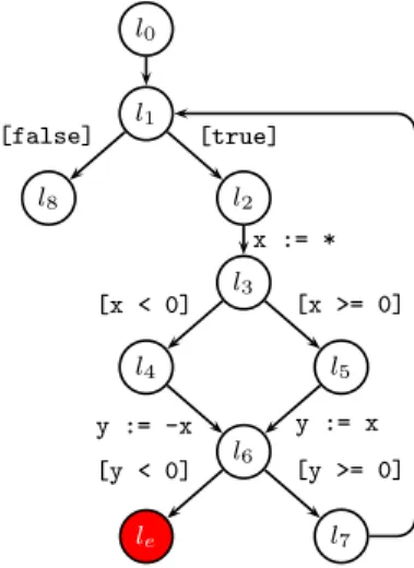
l0 l1 l2 l8 l3 l4 l5 l6 le l7 [true] [false] x := * [x < 0] [x >= 0] y := -x y := x [y >= 0] [y < 0]
Figure 1: An example of acontrol-flow graph.
the assumption that there are no recursive calls (a typical assumption in embedded soft-ware). An assumption is of the form [bexp], where bexp is a Boolean expression that can be a relational operation or an operation involving Boolean operators. Subsequently, we denote byOps the set of program operations.
Without loss of generality, we represent a programP by a control-flow graph (CFG).
Definition 2.1 (Control-Flow Graph). A control-flow graph Gfor a programP is a tuple (L, E, l0, Lerr) where
(1) L is the set of program locations,
(2) E ⊆L×Ops×Lis the set of directed edges labelled by a program operation from the set Ops,
(3) l0 ∈L is the unique entry location such that, for any location l∈L and any operation
op∈Ops, the setE does not contain any edge (l, op, l0), and
(4) Lerr⊆Lof is the set oferror locations such that, for eachle∈Lerr, we have (le, op, l)6∈
E for all op∈Opsand for all l∈L.
In this paper we are interested in verifying safety properties by reducing the verification problem to the reachability of error locations.
Example 2.2. Figure 1 depicts an example of a CFG. Typical program assertions can be represented by branches going to error locations. For example, the branches going out ofl6 can be the representation of assert(y >= 0).
Astate sof a program is a mapping from variables to their values (in this case integers). Let State be the set of states, we have s ∈ State =Var → Z. We denote by Dom(s) the
domain of a state s. We also denote by s[x1 7→ v1, . . . , xn 7→ vn] the state obtained from
s by substituting the image of xi in s by vi for all i = 1, . . . , n. Let G = (L, E, l0, Lerr)
be the CFG for a program P. A configuration γ of P is a pair (l, s), where l ∈ L and s
is a state. We assume some first-order language in which one can represent a set of states symbolically. We write s |= ϕ to mean the formula ϕ is true in the state s, and also say that ssatisfies ϕ, or thatϕ holds at s. A data region r ⊆State is a set of states. A data region r can be represented symbolically by a first-order formula ϕr, with free variables
fromVar, such that all states inr satisfyϕr; that is,r ={s|s|=ϕr}. When the context is clear, we also call the formulaϕr data region as well. Anatomic region, or simply aregion,
is a pair (l, ϕ), where l ∈ L and ϕ is a data region, such that the pair represents the set {(l, s)|s|=ϕ} of program configurations. When the context is clear, we often refer to the both kinds of region as simply region.
The semantics of an operation op∈Ops can be defined by the strongest post-operator SPop. For a formulaϕrepresenting a region, thestrongest post-condition SPop(ϕ) represents
the set of states that are reachable from any of the states in the region represented byϕafter the execution of the operationop. The semantics of assignment and assumption operations are as follows:
SPx:=exp(ϕ) = ∃x′.ϕ[x/x′]∧(x=exp[x/x′]), for exp6=∗,
SPx:=∗(ϕ) = ∃x′.ϕ[x/x′]∧(x=a), whereais a fresh variable, and SP[bexp](ϕ) = ϕ∧bexp,
where ϕ[x/x′
] and exp[x/x′
], respectively, denote the formula obtained from ϕ and the expression obtained fromexp by replacing the variable x′
forx. We define the application of the strongest post-operator to a finite sequence σ = op1, . . . , opn of operations as the successive application of the strongest post-operator to each operator as follows: SPσ(ϕ) = SPopn(. . .SPop1(ϕ). . .).
2.2. Predicate Abstraction. A program can be viewed as a transition system with tran-sitions between configurations. The set of configurations can potentially be infinite because the states can be infinite. Predicate abstraction [GS97] is a technique for extracting a finite transition system from a potentially infinite one by approximating possibly infinite sets of states of the latter system by Boolean combinations of some predicates.
Let Π be a set of predicates over program variables in some quantifier-free theoryT. A
precisionπ is a finite subset of Π. Apredicate abstractionϕπ of a formula ϕover a precision π is a Boolean formula over π that is entailed by ϕ inT, that is, the formula ϕ⇒ ϕπ is
valid inT. To avoid losing precision, we are interested in the strongest Boolean combination
ϕπ, which is called Boolean predicate abstraction [LNO06]. As described in [LNO06], for a
formulaϕ, the more predicates we have in the precisionπ, the more expensive the computa-tion of Boolean predicate abstraccomputa-tion. We refer the reader to [LNO06, CCF+07, CDJR09] for the descriptions of advanced techniques for computing predicate abstractions based on Satisfiability Modulo Theory (SMT) [BSST09].
Given a precisionπ, we can define theabstract strongest post-operator SPπopfor an
oper-ation op. That is, theabstract strongest post-condition SPπop(ϕ) is the formula (SPop(ϕ))π.
2.3. Predicate-Abstraction based Software Model Checking. One prominent soft-ware model checking technique is the lazy predicate abstraction [BHJM07] technique. This technique is a counter-example guided abstraction refinement (CEGAR) [CGJ+03] tech-nique based on on-the-fly construction of an abstract reachability tree (ART). An ART describes the reachable abstract states of the program: a node in an ART is a region (l, ϕ) describing an abstract state. Children of an ART node (orabstract successors) are obtained by unwinding the CFG and by computing the abstract post-conditions of the node’s data region with respect to the unwound CFG edge and some precisionπ. That is, the abstract successors of a node (l, ϕ) is the set {(l1, ϕ1), . . . ,(ln, ϕn)}, where, fori= 1, . . . , n, we have (l, opi, li) is a CFG edge, and ϕi =SPopπii(ϕ) for some precisionπi. The precisionπi can be
associated with the locationli or can be associated globally with the CFG itself. The ART edge connecting a node (l, ϕ) with its child (l′
, ϕ′
CFG edge (l, op, l′
). In this paper computing abstract successors of an ART node is also called node expansion. An ART node (l, ϕ) iscovered by another ART node (l′
, ϕ′
) ifl=l′
andϕentailsϕ′
. A node (l, ϕ) can be expanded if it is not covered by another node and its data region ϕ is satisfiable. An ART is complete if no further node expansion is possible. An ART node (l, ϕ) is anerror node if ϕ is satisfiable andl is an error location. An ART issafe if it is complete and does not contain any error node. Obtaining a safe ART implies that the program is safe.
The construction of an ART for a the CFGG= (L, E, l0, Lerr) for a program P starts
from its root (l0,⊤). During the construction, when an error node is reached, we check if the path from the root to the error node is feasible. An ART path ρ is a finite sequence
ε1, . . . , εn of edges in the ART such that, for every i = 1, . . . , n−1, the target node of εi is the source node ofεi+1. Note that, the ART path ρ corresponds to a path in the CFG. We denote by σρ the sequence of operations labelling the edges of the ART path ρ. A
counter-example path is an ART pathε1, . . . , εnsuch that the source node of ε1 is the root of the ART and the target node ofεn is an error node. A counter-example pathρisfeasible
if and only if SPσρ(true) is satisfiable. An infeasible counter-example path is also called
spurious counter-example. A feasible counter-example path witnesses that the programP
is unsafe.
An alternative way of checking feasibility of a counter-example path ρ is to create a
path formula that corresponds to the path. This is achieved by first transforming the se-quence σρ = op1, . . . , opn of operations labelling ρ into its single-static assignment (SSA) form [CFR+91], where there is only one single assignment to each variable. Next, a con-straint for each operation is generated by rewriting each assignment x := exp into the equalityx =exp, with nondeterministic construct∗ being translated into a fresh variable, and turning each assumption [bexp] into the constraint bexp. The path formula is the con-junction of the constraint generated by each operation. A counter-example pathρis feasible if and only if its corresponding path formula is satisfiable.
Example 2.3. Suppose that the operations labelling a counter-example path are
x:=y, [x>0], x:=x+1, y:=x, [y<0],
then, to check the feasibility of the path, we check the satisfiability of the following formula:
x1=y0∧x1 >0∧x2 =x1+1∧y1=x2∧y1<0.
If the counter-example path is infeasible, then it has to be removed from the constructed ART by refining the precisions. Such a refinement amounts to analyzing the path and extracting new predicates from it. One successful method for extracting relevant predicates at certain locations of the CFG is based on the computation of Craig interpolants [Cra57], as shown in [HJMM04]. Given a pair of formulas (ϕ−
, ϕ+) such thatϕ−
∧ϕ+ is unsatisfiable, a Craig interpolant of (ϕ−
, ϕ+) is a formula ψ such that ϕ− ⇒
ψ is valid, ψ ∧ϕ+ is unsatisfiable, and ψ contains only variables that are common to both ϕ−
and ϕ+. Given an infeasible counter-example ρ, the predicates can be extracted from interpolants in the following way:
(1) Letσρ=op1, . . . , opn, and let the sub-pathσρi,j such thati≤jdenote the sub-sequence opi, opi+1, . . . , opj ofσρ.
(2) For every k = 1, . . . , n−1, let ϕ1,k be the path formula for the sub-path σ1,k
ρ and
ϕk+1,n be the path formula for the sub-path σk+1,n
ρ , we generate an interpolant ψk of
Scheduler Primitive
Functions
update/query scheduler state
Thread Thread query result get state
set state pass control ... Threaded sequential program T1 TN
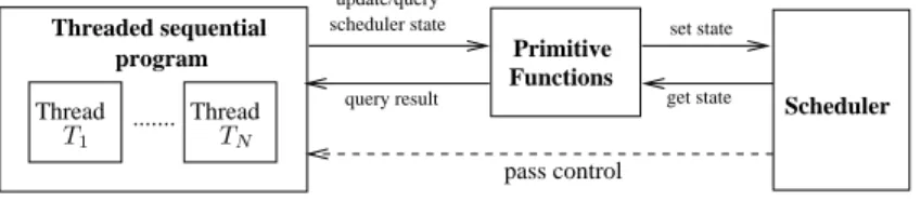
Figure 2: Programming model.
(3) The predicates are the (un-SSA) atoms in the interpolant ψk fork= 1, . . . , n.
The discovered predicates are then added to the precisions that are associated with some locations in the CFG. Letpbe a predicate extracted from the interpolantψkof (ϕ1,k, ϕk+1,n)
for 1≤k < n. Letε1, . . . , εnbe the sequence of edges labelled by the operationsop1, . . . , opn, that is, for i= 1, . . . , n, the edge εi is labelled by opi. Let the nodes (l, ϕ) and (l′, ϕ′) be the source and target nodes of the edge εk. The predicate p can be added to the precision associated with the location l′
.
Once the precisions have been refined, the constructed ART is analyzed to remove the sub part containing the infeasible counter-example path, and then the ART is reconstructed using the refined precisions.
Lazy predicate abstraction has been implemented in several software model checkers, including Blast [BHJM07], CpaChecker [BK11], and Kratos [CGM+11]. For details and in-depth illustrations of ART constructions, we refer the reader to [BHJM07].
3. Programming Model
In this paper we analyze shared-variable multi-threaded programs with exclusive thread
(there is at most one running thread at a time) and cooperative scheduling policy (the scheduler never preempts the running thread, but waits until the running thread coopera-tively yields the control back to the scheduler). At the moment we do not deal with dynamic thread creations. This restriction is not severe because typically multi-threaded programs for embedded system designs are such that all threads are known and created a priori, and there are no dynamic thread creations.
Our programming model is depicted in Figure 2. It consists of three components: a so-called threaded sequential program, a scheduler, and a set of primitive functions. Athreaded sequential program (orthreaded program) P is a multi-threaded program consisting of a set of sequential programsT1, . . . , TN such that each sequential programTi represent athread. From now on, we will refer to the sequential programs in the threaded programs as threads. We assume that the threaded program has a main thread, denoted by main, from which the execution starts. The main thread is responsible for initializing the shared variables.
LetP be a threaded program, we denote byGVar the set of shared (or global) variables of P and by LVarT the set of local variables of the thread T in P. We assume that LVarT ∩GVar =∅ for every thread T and LVarTi ∩LVarTj = ∅ for each two threads Ti
and Tj such thati6=j. We denote byGT the CFG for the thread T. All operations in GT
only access variables inLVarT ∪GVar.
The scheduler governs the executions of threads. It employs a cooperative scheduling policy that only allows at most one running thread at a time. The scheduler keeps track of a set of variables that are necessary to orchestrate the thread executions and synchronizations. We denote such a set by SVar. For example, the scheduler can keep track of the states
of threads and events, and also the time delays of event notifications. The mapping from variables inSVar to their values form ascheduler state. Passing the control to a thread can be done, for example, by simply setting the state of the thread to running. Such a control passing is represented by the dashed line in Figure 2.
Primitive functions are special functions used by the threads to communicate with the scheduler by querying or updating the scheduler state. To allow threads to call primitive functions, we simply extend the form of assignment described in Section 2.1 as follows: the expression exp of an assignment x := exp can also be a call to a primitive function. We assume that such a function call is the top-level expression exp and not nested in another expression. Calls to primitive functions do not modify the values of variables occurring in the threaded program. Note that, as primitive function calls only occur on the right-hand side of assignment, we implicitly assume that every primitive function has a return value.
The primitive functions can be thought of as a programming interface between the threads and the scheduler. For example, for event-based synchronizations, one can have a primitive function wait event(e) that is parametrized by an event name e. This function suspends the calling thread by telling the scheduler that it is now waiting for the notification of event e. Another example is the function notify event(e)that triggers the notification of event e by updating the event’s state, which is tracked by the scheduler, to a value indicating that it has been notified. In turn, the scheduler can wake up the threads that are waiting for the notification ofeby making them runnable.
We now provide a formal semantics for our programming model. Evaluating expressions in program operations involves three kinds of state:
(1) The statesi of local variables of some thread Ti (Dom(si) =LVarTi).
(2) The stategs of global variables (Dom(gs) =GVar). (3) Thescheduler state S (Dom(S) =SVar).
The evaluation of the right-hand side expression of an assignment requires a scheduler state because the expression can be a call to a primitive function whose evaluation depends on and can update the scheduler state.
We require, for each threadT, there is a variablestT ∈Dom(S) that indicates the state
of T. We consider the set{Running,Runnable,Waiting}as the domain of stT, where each
element in the set has an obvious meaning. The elementsRunning,Runnable, andWaiting
can be thought of as enumerations that denote different integers. We say that the thread
T isrunning,runnable, orwaiting in a scheduler state Sif S(stT) is, respectively, Running, Runnable, orWaiting. We denote bySState the set of all scheduler states. Given a threaded program withN threadsT1, . . . , TN, by the exclusive running thread property, we have, for every state S∈SState, if, for somei, we haveS(stT
i) =Running, thenS(stTj) 6=Running
for all j6=i, where 1≤i, j≤N.
The semantics of expressions in program operations are given by the following two evaluation functions
[[·]]E : exp→((State×State×SState)→(Z×SState))
[[·]]B : bexp→((State×State×SState)→ {true, f alse}).
The function [[·]]E takes as arguments an expression occurring on the right-hand side of
an assignment and the above three kinds of state, and returns the value of evaluating the expression over the states along with the possible updated scheduler state. The function [[·]]B takes as arguments a boolean expression and the local and global states, and returns
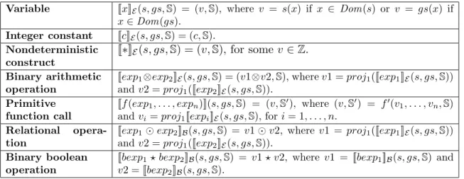
Variable [[x]]E(s, gs,S) = (v,S), where v = s(x) if x ∈ Dom(s) or v = gs(x) if x∈Dom(gs). Integer constant [[c]]E(s, gs,S) = (c,S). Nondeterministic construct [[∗]]E(s, gs,S) = (v,S), for somev∈Z. Binary arithmetic operation
[[exp1⊗exp2]]E(s, gs,S) = (v1⊗v2,S), wherev1 =proj1([[exp1]]E(s, gs,S))
andv2 =proj1([[exp2]]E(s, gs,S)). Primitive
function call
[[f(exp1, . . . , expn)]](s, gs,S) = (v,S′), where (v,S′) = f′(v1, . . . , vn,S)
andvi =proj1[[expi]]E(s, gs,S), fori= 1, . . . , n.
Relational
opera-tion
[[exp1⊙exp2]]B(s, gs,S) = v1⊙v2, where v1 = proj1([[exp1]]E(s, gs,S))
andv2 =proj1([[exp2]]E(s, gs,S)). Binary boolean
operation
[[bexp1⋆ bexp2]]B(s, gs,S) = v1⋆ v2, where v1 = [[bexp1]]B(s, gs,S) and
v2 = [[bexp2]]B(s, gs,S).
Figure 3: Semantics of expressions in program operations.
program operations given by the evaluation functions [[·]]E and [[·]]B. To extract the result
of evaluation function, we use the standard projection functionproji to get the i-th value of a tuple. The rules for unary arithmetic operations and unary boolean operations can be defined similarly to their binary counterparts. For primitive functions, we assume that everyn-ary primitive functionf is associated with an (n+ 1)-ary functionf′
such that the first narguments off′
are the values resulting from the evaluations of the arguments of f, and the (n+ 1)-th argument of f′
is a scheduler state. The function f′
returns a pair of value and updated scheduler state.
Next, we define the meaning of a threaded program by using the operational semantics in terms of the CFGs of the threads. The main ingredient of the semantics is the notion of run-time configuration. Let GT = (L, E, l0, Lerr) be the CFG for a threadT. A thread configuration γT ofT is a pair (l, s), wherel∈Landsis a state such thatDom(s) =LVarT. Definition 3.1(Configuration). Aconfiguration γof a threaded programP withN threads
T1, . . . , TN is a tuple hγT1, . . . , γTN, gs,Si where
• each γTi is a thread configuration of thread Ti,
• gsis the state of global variables, and • Sis the scheduler state.
For succinctness, we often refer the thread configurationγTi = (l, s) of the threadTi as
the indexed pair (l, s)i. A configuration hγT1, . . . , γTN, gs,Si, is an initial configuration for
a threaded program if for eachi= 1, . . . , N, the location lof γTi = (l, s) is the entry of the
CFGGTi of Ti, and S(stmain) =Running and S(stTi)6=Running for all Ti 6=main.
LetSStateN o ⊂SState be the set of scheduler states such that every state inSStateN o
has no running thread, and SStateOne ⊂ SState be the set of scheduler states such that
every state in SStateOne has exactly one running thread. A scheduler with a cooperative scheduling policy can simply be defined as a function Sched :SStateN o→ P(SStateOne).
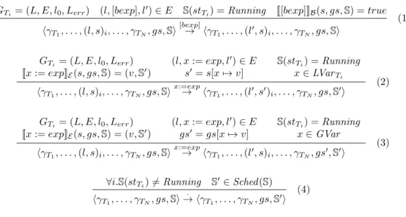
The transitions of the semantics are of the form
Edge transition: γ →op γ′
Scheduler transition: γ →· γ′
whereγ, γ′
are configurations and opis the operation labelling an edge. Figure 4 shows the semantics of threaded programs. The first three rules show that transitions over edges of the
GTi = (L, E, l0, Lerr) (l,[bexp], l′)∈E S(stTi) =Running [[[bexp]]]B(s, gs,S) =true hγT1, . . . ,(l, s)i, . . . , γTN, gs,Si [bexp] → hγT1, . . . ,(l′, s)i, . . . , γTN, gs,Si (1) GTi = (L, E, l0, Lerr) [[x:=exp]]E(s, gs,S) = (v,S′) (l, x:=exp, l′ )∈E s′ =s[x7→v] S(stTi) =Running x∈LVarTi hγT1, . . . ,(l, s)i, . . . , γTN, gs,Si x:=exp → hγT1, . . . ,(l′, s′)i, . . . , γTN, gs,S′i (2) GTi = (L, E, l0, Lerr) [[x:=exp]]E(s, gs,S) = (v,S′) (l, x:=exp, l′ )∈E gs′ =gs[x7→v] S(stTi) =Running x∈GVar hγT1, . . . ,(l, s)i, . . . , γTN, gs,Si x:=exp → hγT1, . . . ,(l′, s)i, . . . , γTN, gs′,S′i (3) ∀i.S(stTi)6=Running S′ ∈ Sched(S) hγT1, . . . , γTN, gs,Si · → hγT1, . . . , γTN, gs,S ′i (4)
Figure 4: Operational semantics of threaded sequential programs.
CFGGT of a thread T are defined if and only ifT is running, as indicated by the scheduler state. The first rule shows that a transition over an edge labelled by an assumption is defined if the boolean expression of the assumption evaluates to true. The second and third rules show the updates of the states caused by the assignment. Finally, the fourth rule describes the running of the scheduler.
Definition 3.2 (Computation Sequence, Run, Reachable Configuration). A computation sequence γ0, γ1, . . . of a threaded program P is either a finite or an infinite sequence of configurations ofP such that, for all i, eitherγi →op γi+1 for some operationopor γi
·
→γi+1. A run of a threaded program P is a computation sequence γ0, γ1, . . . such that γ0 is an initial configuration. A configuration γ of P is reachable from a configuration γ′
if there is a computation sequence γ0, . . . , γn such that γ0 = γ′ and γn =γ. A configuration γ is
reachable in P if it is reachable from an initial configuration.
A configuration hγT1, . . . ,(l, s)i, . . . , γTN, gs,Si of a threaded program P is an error
configuration if CFG GTi = (L, E, l0, Lerr) andl ∈Lerr. We say a threaded programP is
safe iff no error configuration is reachable in P; otherwise, P is unsafe. 4. Explicit-Scheduler Symbolic-Thread (ESST)
In this section we present our novel technique for verifying threaded programs. We call our technique Explicit-Scheduler Symbolic-Thread (ESST) [CMNR10]. This technique is a CEGAR based technique that combines explicit-state techniques with the lazy predicate abstraction described in Section 2.3. In the same way as the lazy predicate abstraction, ESST analyzes the data path of the threads by means of predicate abstraction and ana-lyzes the flow of control of each thread with explicit-state techniques. Additionally, ESST includes the scheduler as part of its model checking algorithm and analyzes the state of the scheduler with explicit-state techniques.
4.1. Abstract Reachability Forest (ARF). The ESST technique is based on the on-the-fly construction and analysis of an abstract reachability forest (ARF). An ARF de-scribes the reachable abstract states of the threaded program. It consists of connected
abstract reachability trees (ARTs), each describing the reachable abstract states of the run-ning thread. The connections between one ART with the others in an ARF describe possible thread interleavings from the currently running thread to the next running thread.
LetP be a threaded program withN threadsT1, . . . , TN. Athread region for the thread
Ti, for 1≤i≤N, is a set of thread configurations such that the domain of the states of the
configurations isLVarTi∪GVar. Aglobal region for a threaded program P is a set of states
whose domain is S
i=1,...,NLVarTi ∪GVar.
Definition 4.1 (ARF Node). An ARF node for a threaded program P with N threads
T1, . . . , TN is a tuple
(hl1, ϕ1i, . . . ,hlN, ϕNi, ϕ,S),
where (li, ϕi), for i= 1, . . . , N, is a thread region for Ti,ϕ is a global region, andS is the
scheduler state.
Note that, by definition, the global region, along with the program locations and the scheduler state, is sufficient for representing the abstract state of a threaded program. However, such a representation will incur some inefficiencies in computing the predicate abstraction. That is, without any thread regions, the precision is only associated with the global region. Such a precision will undoubtedly contains a lot of predicates about the variables occurring in the threaded program. However, when we are interested in computing an abstraction of a thread region, we often do not need the predicates consisting only of variables that are local to some other threads.
In ESSTwe can associate a precision with a location li of the CFG GT for thread T,
denoted byπli, with a threadT, denoted byπT, or the global regionϕ, denoted byπ. For a
precisionπT and for every locationl ofGT, we haveπT ⊆πl for the precisionπlassociated
with the location l. Given a predicate ψ and a location l of the CFG GTi, and let fvar(ψ)
be the set of free variables of ψ, we can add ψinto the following precisions: • Iffvar(ψ)⊆LVarTi, thenψ can be added intoπ,πTi, or πl.
• Iffvar(ψ)⊆LVarTi∪GVar, thenψ can be added intoπ,πTi, orπl.
• Iffvar(ψ)⊆S
j=1,...,NLVarTj ∪GVar, thenψ can be added intoπ.
4.2. Primitive Executor and Scheduler. As indicated by the operational semantics of threaded programs, besides computing abstract post-conditions, we need to execute calls to primitive functions and to explore all possible schedules (or interleavings) during the construction of an ARF. For the calls to primitive functions, we assume that the values passed as arguments to the primitive functions are known statically. This is a limitation of the currentESST algorithm, and we will address this limitation in our future work.
Recall that,SState denotes the set of scheduler states, and letPrimitiveCall be the set of calls to primitive functions. To implement the semantic function [[exp]]E, whereexp is a
primitive function call, we introduce the function
Sexec: (SState×PrimitiveCall)→(Z×SState).
This function takes as inputs a scheduler state, a call f(~x) to a primitive function f, and returns a value and an updated scheduler state resulting from the execution of f on the
arguments~x. That is,Sexec(S, f(~x)) essentially computes [[f(~x)]]E(·,·,S). Since we assume
that the values of ~x are known statically, we deliberately ignore, by ·, the states of local and global variables.
Example 4.2. Let us consider a primitive function call wait event(e) that suspends a running thread T and makes the thread wait for a notification of an event e. Let evT be the variable in the scheduler state that keeps track of the event whose notification is waited for by T. The stateS′ of (·,S′) =Sexec(S,wait event(e)) is obtained from the stateS by
changing the status of running thread toWaiting, and noting that the thread is waiting for event e, that is,S′ =S[sT 7→Waiting, evT 7→e].
Finally, to implement the scheduler function Sched in the operational semantics, and to explore all possible schedules, we introduce the function
Sched:SStateN o → P(SStateOne).
This function takes as an input a scheduler state and returns a set of scheduler states that represent all possible schedules.
4.3. ARF Construction. We expand an ARF node by unwinding the CFG of the running thread and by running the scheduler. Given an ARF node
(hl1, ϕ1i, . . . ,hlN, ϕNi, ϕ,S),
we expand the node by the following rules [CMNR10]:
E1. If there is a running threadTi inS such that the thread performs an operationop and
(li, op, l′
i) is an edge of the CFG GTi of threadTi, then we have two cases:
• Ifop isnot a call to primitive function, then the successor node is (hl1, ϕ′1i, . . . ,hl ′ i, ϕ ′ ii, . . . ,hlN, ϕ′Ni, ϕ ′ ,S), where (i) ϕ′i =SPπl′i op(ϕi∧ϕ) and πl′
i is the precision associated withl
′ i,
(ii) ϕ′ j =SP
πlj
havoc(op)(ϕj ∧ϕ) forj 6=i and πlj is the precision associated with lj,
if op possibly updates global variables, otherwise ϕ′
j =ϕj, and
(iii) ϕ′
=SPπop(ϕ) and π is the precision associated with the global region.
The function havoccollects all global variables possibly updated by op, and builds a new operation where these variables are assigned with fresh variables. The edge connecting the original node and the resulting successor node is labelled by the operationop.
• Ifop is a primitive function call x:=f(~y), then the successor node is (hl1, ϕ′1i, . . . ,hl ′ i, ϕ ′ ii, . . . ,hlN, ϕ ′ Ni, ϕ ′ ,S′), where (i) (v,S′) =Sexec(S, f(~y)), (ii) op′ is the assignment x:=v, (iii) ϕ′ i =SP πl′ i op′(ϕi∧ϕ) and πl′
i is the precision associated withl
′ i,
(iv) ϕ′ j =SP
πlj
havoc(op′)(ϕj ∧ϕ) for j 6=iand πlj is the precision associated withlj
if op possibly updates global variables, otherwise ϕ′
j =ϕj, and
(v) ϕ′
The edge connecting the original node and the resulting successor node is labelled by the operationop′
.
E2. If there is no running thread inS, then, for eachS′ ∈Sched(S), we create a successor
node
(hl1, ϕ1i, . . . ,hlN, ϕNi, ϕ,S′).
We call such a connection between two nodes an ARF connector.
Note that, the rule E1 constructs the ART that belongs to the running thread, while the connections between the ARTs that are established by ARF connectors in the rule E2 represent possible thread interleavings or context switches.
An ARF node (hl1, ϕ1i, . . . ,hlN, ϕNi, ϕ,S) is theinitial node if for alli= 1, . . . , N, the location li is the entry location of the CFGGTi of thread Ti and ϕi istrue,ϕis true, and
S(smain) =Running and S(sT
i)6=Running for all Ti 6=main.
We construct an ARF by applying the rules E1 and E2 starting from the initial node. A node can be expanded if the node is not covered by other nodes and if the conjunction of all its thread regions and the global region is satisfiable.
Definition 4.3 (Node Coverage). An ARF node (hl1, ϕ1i, . . . ,hlN, ϕNi, ϕ,S) iscovered by
another ARF node (hl′
1, ϕ′1i, . . . ,hlN′ , ϕ ′ Ni, ϕ ′ ,S′ ) if li = l′ i for i = 1, . . . , N, S = S ′ , and ϕ⇒ϕ′ andV i=1,...,N(ϕi ⇒ϕ ′ i) are valid.
An ARF is complete if it is closed under the expansion of rules E1 and E2. An ARF node (hl1, ϕ1i, . . . ,hlN, ϕNi, ϕ,S) is an error node if ϕ∧Vi=1,...,Nϕi is satisfiable, and at
least one of the locations l1, . . . , lN is an error location. An ARF is safe if it is complete
and does not contain any error node.
4.4. Counter-example Analysis. Similar to the lazy predicate abstraction for sequential programs, during the construction of an ARF, when we reach an error node, we check if the path in the ARF from the initial node to the error node is feasible.
Definition 4.4 (ARF Path). An ARF path ρˆ=ρ1, κ1, ρ2, . . . , κn−1, ρn is a finite sequence
of ART paths ρi connected by ARF connectors κj, such that (1) ρi, for i= 1, . . . , n, is an ART path,
(2) κj, for j = 1, . . . , n−1, is an ARF connector, and (3) for every j = 1, . . . , n−1, such that ρj = εj1, . . . , ε
j
m and ρj+1 = εj1+1, . . . , ε
j+1
l , the
target node of εjm is the source node of κj and the source node of εj1+1 is the target
node of κj.
A suppressed ARF path sup(ˆρ) of ˆρ is the sequenceρ1, . . . , ρn.
A counter-example path ρˆ is an ARF path such that the source node of ε1 of ρ1 =
ε1, . . . , εm is the initial node, and the target node of ε′k of ρn=ε ′
1, . . . , ε′k is an error node.
Let σsup(ˆρ) denote the sequence of operations labelling the edges in sup(ˆρ). We say that a counter-example path ˆρ isfeasible if and only ifSPσsup( ˆρ)(true) is satisfiable. Similar to the case of sequential programs, one can check the feasibility of ˆρ by checking the satisfiability of the path formula corresponding to the SSA form of σsup(ˆρ).
Example 4.5. Suppose that the top path in Figure 5 is a counter-example path (the target node of the last edge is an error node). The bottom path is the suppressed version of the top one. The dashed edge is an ARF connector. To check feasibility of the path by means of
x := x+y y := 7 x := z [x < y+z]
x := x+y y := 7 x := z [x < y+z]
Suppressed
Figure 5: An example of a counter-example path.
satisfiability of the corresponding path formula, we check the satisfiability of the following formula:
x1=x0+y0∧y1=7∧x2=z0∧x2<y1+z0.
4.5. ARF Refinement. When the counter-example path ˆρ is infeasible, we need to rule out such a path by refining the precision of nodes in the ARF. ARF refinement amounts to finding additional predicates to refine the precisions. Similar to the case of sequential pro-grams, these additional predicates can be extracted from the path formula corresponding to sequenceσsup(ˆρ) by using the Craig interpolant refinement method described in Section 2.3. As described in Section 4.1 newly discovered predicates can be added to precisions associated to locations, threads, or the global region. Consider again the Craig interpolant method in Section 2.3. Let ε1, . . . , εn be the sequence of edges labelled by the operations
op1, . . . , opn of σsup(ˆρ), that is, for i= 1, . . . , n, the edge εi is labelled by opi. Let p be a
predicate extracted from the interpolant ψk of (ϕ1,k, ϕk+1,n) for 1 ≤ k < n, and let the nodes (hl1, ϕ1i, . . . ,hli, ϕii, . . . ,hlN, ϕNi, ϕ,S) and (hl1, ϕ′1i, . . . ,hl ′ i, ϕ ′ ii, . . . ,hlN, ϕ ′ Ni, ϕ ′ ,S′)
be, respectively, the source and target nodes of the edge εk such that the running thread
in the source node’s scheduler state is the thread Ti. If p contains only variables local to
Ti, then we can addp to the precision associated with the location li′, to the the precision
associated with Ti, or to the precision associated with the global region. Other precisions refinement strategies are applicable. For example, one might add a predicate into the precision associated with the global region if and only if the predicate contains variables local to several threads.
Similar to the ART refinement in the case of sequential programs, once the precisions are refined, we refine the ARF by removing the infeasible counter-example path or by removing part of the ARF that contains the infeasible path, and then reconstruct again the ARF using the refined precisions.
4.6. Havocked Operations. Computing the abstract strongest post-conditions with re-spect to the havocked operation in the rule E1 is necessary, not only to keep the regions of the ARF node consistent, but, more importantly, to maintain soundness: never reports safe for an unsafe case. Suppose that the region of a non-running threadT is the formulax=g, wherex is a variable local toT and g is a shared global variable. Suppose further that the global region is true. If the running thread T′
updates the value of g with, for example, the assignment g:= w, for some variable w local to T′
no longer hold, and has to be invalidated. Otherwise, when T resumes, and, for example, checks for an assertion assert(x=g), then no assertion violation can occur. One way to keep the region ofT consistent is to update the region using the havoc(g:=w) operation, as shown in the rule E1. That is, we compute the successor region of T asSPπl
g:=a(x=g),
whereais a fresh variable andlis the current location ofT. The fresh variableaessentially denotes an arbitrary value that is assigned tog.
Note that, by using ahavoc(op) operation, we do not leak variables local to the running thread when we update the regions of non-running threads. Unfortunately, the use of havoc(op) can cause loss of precision. One way to address this issue is to add predicates containing local and global variables to the precision associated with the global region. An alternative approach, as described in [DKKW11], is to simply use the operationop(leaking the local variables) when updating the regions of non-running threads.
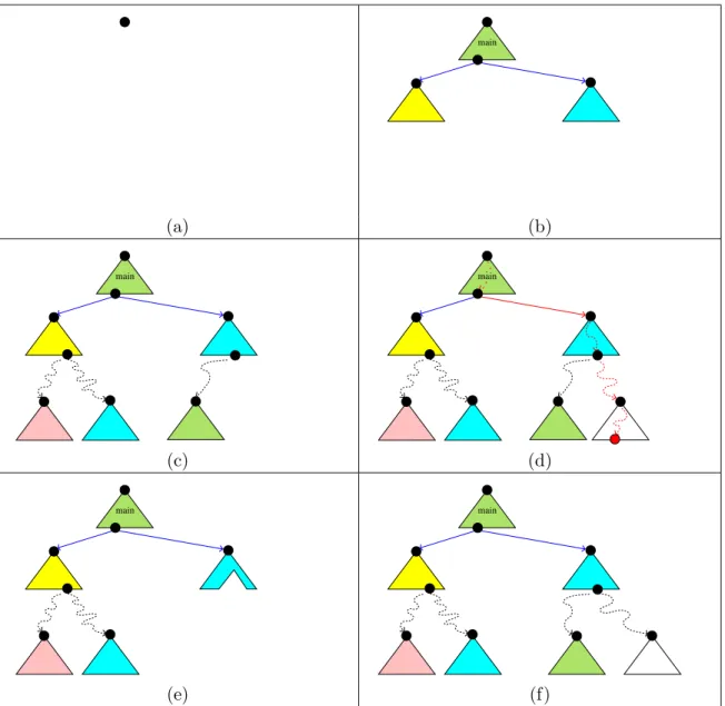
4.7. Summary of ESST. The ESST algorithm takes a threaded programP as an input and, when its execution terminates, returns either a feasible counter-example path and reports that P is unsafe, or a safe ARF and reports that P is safe. The execution of ESST(P) can be illustrated in Figure 6:
(1) Start with an ARF consisting only of the initial node, as shown in Figure 6(a).
(2) Pick an ARF node that can be expanded and apply the rules E1 or E2 to grow the ARF, as shown in Figures 6(b) and 6(c). The different colors denote the different threads to which the ARTs belong.
(3) If we reach an error node, as shown by the red line in Figure 6(d), we analyze the counter-example path.
(a) If the path is feasible, then report that P isunsafe. (b) If the path is spurious, then refine the ARF:
(i) Discover new predicates to refine abstractions. (ii) Undo part of the ARF, as shown in Figure 6(e). (iii) Goto (2) to reconstruct the ARF.
(4) If the ARF is safe, as shown in Figure 6(f), then report that P issafe.
4.8. Correctness of ESST. To prove the correctness of ESST, we need to introduce several notions and notations that relate theESSTalgorithm with the operational semantics in Section 3. Given two states s1 and s2 whose domains are disjoint, we denote by s1∪s2 the union of two states such that Dom(s1 ∪s2) is Dom(s1) ∪Dom(s2), and, for every
x∈Dom(s1∪s2), we have
(s1∪s2)(x) =
s1(x) ifx∈Dom(s1);
s2(x) otherwise.
LetP be a threaded program withN threads, and γ be a configuration h(l1, s1), . . . ,(lN, sN), gs,Si,
of P. Letη be an ARF node
(hl′1, ϕ1i, . . . ,hl′N, ϕNi, ϕ,S ′
),
forP. We say that the configuration γ satisfies the ARF nodeη, denoted by γ |=η if and only if for all i = 1, . . . , N, we have li = l′
i and si∪gs |= ϕi,
S
i=1,...,Nsi∪gs |= ϕ, and S=S′.
main (a) (b) main main (c) (d) main main (e) (f)
Figure 6: ARF construction inESST.
By the above definition, it is easy to see that, for any initial configuration γ0 ofP, we have γ0 |=η0 for the initial ARF node η0. In the sequel we refer to the configurations of
P and the ARF nodes (or connectors) forP when we speak about configurations and ARF nodes (or connectors), respectively.
We now show that the node expansion rules E1 and E2 create successor nodes that are over-approximations of the configurations reachable by performing operations considered in the rules.
Lemma 4.6. Letηandη′
be ARF nodes for a threaded programP such thatη′
is a successor node of η. Let γ be a configuration of P such thatγ |=η. The following properties hold:
(1) If η′ is obtained from η by the rule E1 with the performed operation op, then, for any configuration γ′
of P such thatγ →op γ′
, we have γ′
|=η′ .
(2) If η′
is obtained from η by the rule E2, then, for any configuration γ′
of P such that γ →· γ′
and the scheduler states of η′
and γ′
coincide, we have γ′
|=η′ .
Letεbe an ART edge with source node
η= (hl1, ϕ1i, . . . ,hli, ϕii, . . .hlN, ϕNi, ϕ,S) and target node
η′ = (hl1, ϕ′1i, . . . ,hl ′ i, ϕ ′ ii, . . .hlN, ϕ ′ Ni, ϕ ′ ,S′), such that S(sT
i) = Running and for all j 6= i, we have S(sTj) 6= Running. Let GTi =
(L, E, l0, Lerr) be the CFG for Ti such that (li, op, l′i)∈E. Let γ and γ ′ be configurations. We denote by γ →ε γ′ if γ |= η, γ′ |= η′ , and γ →op γ′
. Note that, the operation op is the operation labelling the edge of CFG, not the one labelling the ART edge ε. Similarly, we denote byγ →κ γ′
for an ARF connectorκ ifγ |=η,γ′|
=η′
, andγ →· γ′
. Let ˆρ=ξ1, . . . , ξm be an ARF path. That is, for eachi= 1, . . . , m, the element ξi is either an ART edge or an ARF connector. We denote by γ →ρˆ γ′
if there exists a computation sequenceγ1, . . . , γm+1 such thatγi
ξi
→γi+1 for alli= 1, . . . , m, and γ=γ1 and γ′ =γm+1.
In Section 3 the notion of strongest post-condition is defined as a set of reachable states after executing some operation. We now try to relate the notion of configuration with the notion of strongest post-condition. Letγ be a configuration
γ =h(l1, s1), . . . ,(li, si), . . . ,(lN, sN), gs,Si, and ϕbe a formula whose free variables range overS
k=1,...,NDom(sk)∪Dom(gs). We say
that the configuration satisfies the formula ϕ, denoted by γ |=ϕ if S
k=1,...,Nsk∪gs|=ϕ.
Suppose that in the above configurationγ we haveS(sT
i) =Running andS(sTj)6=Running
for allj 6=i. Let GTi = (L, E, l0, Lerr) be the CFG for Ti such that (li, op, l
′
i) ∈E. Let ˆop
beopif opdoes not contain any primitive function call, otherwise ˆopbeop′
as in the second case of the expansion rule E1. Then, for any configuration
γ′=h(l1, s1), . . . ,(l′i, s ′ i), . . . ,(lN, sN), gs ′ ,S′i, such that γ →op γ′ , we have γ′
|=SPopˆ(ϕ). Note that, the scheduler states S and S′ are not constrained by, respectively, ϕand SPopˆ(ϕ), and so they can be different.
When ESST(P) terminates and reports that P is safe, we require that, for every configurationγ reachable inP, there is a node inF such that the configuration satisfies the node. We denote byReach(P) the set of configurations reachable inP, and by Nodes(F) the set of nodes in F.
Theorem 4.7(Correctness). LetP be a threaded program. For every terminating execution of ESST(P), we have the following properties:
(1) If ESST(P) returns a feasible counter-example path ρ, then we haveˆ γ →ρˆ γ′
for an initial configuration γ and an error configuration γ′ of P.
(2) If ESST(P) returns a safe ARF F, then for every configuration γ ∈ Reach(P), there is an ARF node η ∈Nodes(F) such thatγ |=η.
5. ESST + Partial-Order Reduction
The ESSTalgorithm often has to explore a large number of possible thread interleavings. However, some of them might be redundant because the order of interleavings of some threads is irrelevant. Given N threads such that each of them accesses a disjoint set of variables, there are N! possible interleavings that ESST has to explore. The constructed ARF will consists of 2N abstract states (or nodes). Unfortunately, the more abstract states
to explore, the more computations of abstract strongest post-conditions are needed, and the more coverage checks are involved. Moreover, the more interleavings to explore, the more possible spurious counter-example paths to rule out, and thus the more refinements are needed. As refinements result in keeping track of additional predicates, the computations of abstract strongest post-conditions become expensive. Consequently, exploring all possible interleavings degrades the performance of ESST and leads to state explosion.
Partial-order reduction techniques (POR) [God96, Pel93, Val91] have been successfully applied in explicit-state software model checkers likeSPIN[Hol05] andVeriSoft[God05] to avoid exploring redundant interleavings. PORhas also been applied to symbolic model checking techniques as shown in [KGS06, WYKG08, ABH+01]. In this section we will extend the ESST algorithm with POR techniques. However, as we will see, such an integration is not trivial because we need to ensure that in the construction of the ARF the POR techniques do not make ESSTunsound.
5.1. Partial-Order Reduction (POR). Partial-order reduction (POR) is a model check-ing technique that is aimed at combatcheck-ing the state explosion by explorcheck-ing only represen-tative subset of all possible interleavings. POR exploits the commutativity of concurrent transitions that result in the same state when they are executed in different orders.
We presentPOR using the standard notions and notations used in [God96, CGP99]. We model a concurrent program as a transition systemM = (S, S0, T), whereS is the finite set of states, S0 ⊂S is the set of initial states, and T is a set of transitions such that for each α ∈ T, we have α ⊂ S×S. We say that α(s, s′
) holds and often write it as s →α s′
if (s, s′
)∈α. A state s′
is a successor of a state s if s→α s′
for some transition α ∈T. In the following we will only consider deterministic transitions, and often write s′
=α(s) for
α(s, s′
). A transition α isenabled in a state sif there is a states′
such thatα(s, s′
) holds. The set of transitions enabled in a state sis denoted byenabled(s). Apath from a states
in a transition system is a finite or infinite sequence s0 α0→s1 → · · ·α1 such thats= s0 and
si αi
→ si+1 for all i. A path is empty if the sequence consists only of a single state. The length of a finite path is the number of transitions in the path.
Let M = (S, S0, T) be a transition system, we denote by Reach(S0, T) ⊆S the set of states reachable from the states inS0 by the transitions inT: for a states∈Reach(S0, T), there is a finite paths0
α0
→. . .α→n−1snsystem such thats0 ∈S0 ands=sn. In this work we are interested in verifying safety properties in the form of program assertion. To this end, we assume that there is a set Terr ⊆T of error transitions such that the set
EM,Terr ={s∈S | ∃s
′
∈S.∃α ∈Terr. α(s ′
, s) holds}
is the set of error states ofM with respect to Terr. A transition system M = (S, S0, T) is
Selective search in POR exploits the commutativity of concurrent transitions. The concept of commutativity of concurrent transitions can be formulated by defining an inde-pendence relation on pairs of transitions.
Definition 5.1 (Independence Relation, Independent Transitions). An independence rela-tion I ⊆T×T is a symmetric, anti-reflexive relation such that for each states∈S and for each (α, β)∈I the following conditions are satisfied:
Enabledness: Ifα is in enabled(s), then β is inenabled(s) iffβ is inenabled(α(s)).
Commutativity: If α and β are in enabled(s), then α(β(s)) =β(α(s)).
We say that two transitions αand β areindependent of each other if for every state sthey satisfy the enabledness and commutativity conditions. We also say that two transitions
α and β are independent in a state s of each other if they satisfy the enabledness and commutativity conditions ins.
In the sequel we will use the notion of valid dependence relation to select a representative subset of transitions that need to be explored.
Definition 5.2 (Valid Dependence Relation). A valid dependence relation D ⊆T ×T is a symmetric, reflexive relation such that for every (α, β)6∈D, the transitions α and β are independent of each other.
5.1.1. The Persistent Set Approach. To reduce the number of possible interleavings, in every state visited during the state space exploration one only explores a representative subset of transitions that are enabled in that state. However, to select such a subset we have to avoid possible dependencies that can happen in the future. To this end, we appeal to the notion of persistent set [God96].
Definition 5.3(Persistent Set). A setP ⊆T of enabled transitions in a statesispersistent
insif for every finite non-empty path s=s0→α0 s1 → · · ·α1
αn−1
→ sn αn
→sn+1 such thatαi 6∈P
for all i= 0, . . . , n, we haveαn independent of any transition inP insn.
Note that the persistent set in a state is not unique. To guarantee the existence of successor state, we impose thesuccessor-state condition on the persistent set: the persistent set in s is empty iff so is enabled(s). In the sequel we assume persistent sets satisfy the successor-state condition. We say that a state s is fully expanded if the persistent set in s
equals enabled(s). It is easy to see that, for any transition α not in the persistent set P in a state s, the transition α is disabled ins or independent of any transition inP.
We denote by Reachred(S0, T) ⊆ S the set of states reachable from the states in S0 by the transitions in T such that, during the state space exploration, in every visited state we only explore the transitions in the persistent set in that state. That is, for a state
s ∈ Reachred(S0, T), there is a finite path s0 →α0 . . .
αn−1
→ sn in the transition system such thats0 ∈S0 ands=sn, andαi is in the persistent set of si, for i= 0, . . . , n−1. It is easy to see that Reachred(S0, T)⊆Reach(S0, T).
To preserve safety properties of a transition system, we need to guarantee that the reduction by means of persistent sets does not remove all interleavings that lead to an error state. To this end, we impose thecycle condition onReachred(S0, T) [CGP99, Pel93]: a cycle is not allowed if it contains a state in which a transition α is enabled, but α is never included in the persistent set of any state s on the cycle. That is, if there is a cycle
s0 →α0 . . .
αn−1
→ sn=s0 induced by the states s0, . . . , sn−1 inReachred(S0, T) such that αi is
persistent insi, for i= 0, . . . , n−1 and α ∈enabled(sj) for some 0≤j < n, then α must be in the persistent set of any ofs0, . . . , sn−1.
Theorem 5.4. A transition system M = (S, S0, T) is safe w.r.t. a set Terr ⊆T of error transitions iff Reachred(S0, T) that satisfies the cycle condition does not contain any error
state from EM,Terr.
5.1.2. The Sleep Set Approach. The sleep set POR technique exploits independencies of enabled transitions in the current state. For example, suppose that in some state s there are two enabled transitions α and β, and they are independent of each other. Suppose further that the search explores α first from s. Then, when the search explores β from
s such that s →β s′
for some state s′
, we associate with s′
a sleep set containing only α. From s′
the search only explores transitions that are not in the sleep set of s′
. That is, although the transition α is still enabled in s′, it will not be explored. Both persistent set and sleep set techniques are orthogonal and complementary, and thus can be applied simultaneously. Note that the sleep set technique only removes transitions, and not states. Thus, Theorem 5.4 still holds when the sleep set technique is applied.
5.2. Applying POR to ESST. The key idea of applying POR to ESST is to select a representative subset of scheduler states output by the scheduler inESST. That is, instead of creating successor nodes with all scheduler states from{S1, . . . ,Sn}=Sched(S), for some
state S, we create successor nodes with the representative subset of{S1, . . . ,Sn}. However,
such an application is non-trivial. The ESST algorithm is based on the construction of an ARF that describes the reachable abstract states, while the exposition of POR before is based on the analysis of reachable concrete states. As we will see later, some POR properties that hold in the concrete state space do not hold in the abstract state space. Nevertheless, in applying POR to ESST one needs to guarantee that the original ARF is safe if and only if the reduced ARF, obtained by the restriction on the scheduler’s output, is safe. In particular, the construction of reduced ARF has to check if the cycle condition is satisfied in its concretization.
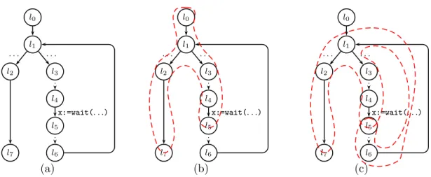
To integrate PORtechniques into the ESST algorithm, we first need to identify frag-ments in the threaded program that count as transitions in the transition system. In the previous description of POR the execution of a transition is atomic, that is, its execution cannot be interleaved by the executions of other transitions. We introduce the notion of atomic block as the notion of transition in the threaded program. Intuitively, an atomic block is a block of operations between calls to primitive functions that can suspend the thread. Let us call such primitive functionsblocking functions.
An atomic block of a thread is a rooted subgraph of the CFG such that the subgraph satisfies the following conditions:
(1) its unique entry is the entry of the CFG or the location that immediately follows a call to a blocking function;
(2) its exit is the exit of the CFG or the location that immediately follows a call to a blocking function; and
(3) there is no call to a blocking function in any CFG path from the entry to an exit except the one that precedes the exit.
l0 l1 l2 l3 l4 l5 l6 l7 . . . . x:=wait(. . .) l0 l1 l2 l3 l4 l5 l6 l7 . . . . x:=wait(. . .) l0 l1 l2 l3 l4 l5 l6 l7 . . . . x:=wait(. . .) (a) (b) (c)
Figure 7: Identifying atomic blocks.
Note that an atomic block has a unique entry, but can have multiple exits. We often identify an atomic block by its entry. Furthermore, we denote by ABlock the set of atomic blocks.
Example 5.5. Consider a thread whose CFG is depicted in Figure 7(a). Letwait(. . .)be the only call to a blocking function in the CFG. Figures 7(b) and (c) depicts the atomic blocks of the thread. The atomic block in Figure 7(b) starts from l0 and exits atl5 andl7, while the one in Figure 7(c) starts from l5 and exits at l5 and l7.
Note that, an atomic block can span over multiple basic blocks or even multiple large blocks in the basic block or large block encoding [BCG+09]. In the sequel we will use the terms transition and atomic block interchangeably.
Prior to computing persistent sets, we need to compute valid dependence relations. The criteria for two transitions being dependent are different from one application domain to the other. Cooperative threads in many embedded system domains employ event-based synchronizations through event waits and notifications. Different domains can have different types of event notification. For generality, we anticipate two kinds of notification: immediate and delayed notifications. An immediate notification is materialized immediately at the current time or at the current cycle (for cycle-based semantics). Threads that are waiting for the notified events are made runnable upon the notification. A delayed notification is scheduled to be materialized at some future time or at the end of the current cycle. In some domains delayed notifications can be cancelled before they are triggered.
For example, in a system design language that supports event-based synchronization, a pair (α, β) of atomic blocks are in a valid dependence relation if one of the following criteria is satisfied: (1) the atomic block α contains a write to a shared (or global) variable g, and the atomic block β contains a write or a read to g; (2) the atomic block α contains an immediate notification of an evente, and the atomic blockβ contains a wait for e; (3) the atomic blockαcontains a delayed notification of an evente, and the atomic blockβcontains a cancellation of a notification ofe. Note that the first criterion is a standard criterion for two blocks to become dependent on each other. That is, the order of executions of the two blocks is relevant because different orders yield different values assigned to variables. The second and the third criteria are specific to event-based synchronization language. An event notification can make runnable a thread that is waiting for a notification of the event. A waiting thread misses an event notification if the thread waited for such a notification
Algorithm 1 Persistent sets.
Input: a set Benof enabled atomic blocks. Output: a persistent setP.
(1) LetB :={α}, where α∈Ben. (2) For each atomic blockα∈B:
(a) If α∈Ben (α is enabled):
• Add into B every atomic block β such that (α, β) ∈D. (b) Ifα6∈Ben (α is disabled):
• Add into B a necessary enabling set forα with Ben. (3) Repeat step 2 until no more atomic blocks can be added into B. (4) P :=B∩Ben.
after another thread had made the notification. Thus, the order of executions of atomic blocks containing event waits and event notifications is relevant. Similarly for the delayed notification in the third criterion. Given criteria for being dependent, one can use static analysis techniques to compute a valid dependence relation.
To have small persistent sets, we need to know whether a disabled transition that has a dependence relation with the currently enabled ones can be made enabled in the future. To this end, we use the notion of necessary enabling set introduced in [God96].
Definition 5.6 (Necessary Enabling Set). Let M = (S, S0, T) be a transition system such that a transition α∈T is diabled in a state s∈S. A set Tα,s ⊆T is a necessary enabling set for α in s if for every finite path s=s0 → · · ·α0
αn−1
→ sn in M such that α is disabled in
si, for all 0 ≤i < n, but is enabled in sn, a transition tj, for some 0 ≤ j ≤ n−1, is in
Tα,s. A setTα,Ten ⊆T, forTen⊆T, is anecessary enabling set for α with Ten if Tα,Ten is a
necessary enabling set for α in every state ssuch thatTen is the set of enabled transitions ins.
Intuitively, a necessary enabling setTα,sfor a transitionα in a statesis a set of transitions such that α cannot become enabled in the future before at least a transition in Tα,s is executed.
Algorithm 1 computes persistent sets using a valid dependence relationD. It is easy to see that the persistent set computed by the algorithm satisfies the successor-state condition. The algorithm is also a variant of the stubborn set algorithm presented in [God96], that is, we use a valid dependence relation as the interference relation used in the latter algorithm. We applyPORto theESSTalgorithm by modifying the ARF node expansion rule E2, described in Section 4 in two steps. First we compute a persistent set from a set of scheduler states output by the functionSched. Second, we ensure that the cycle condition is satisfied by the concretization of the constructed ARF.
We introduce the functionPersistentthat computes a persistent set of a set of sched-uler states. Persistenttakes as inputs an ARF node and a set S of scheduler states, and outputs a subset S′
of S. The input ARF node keeps track of the thread locations, which are used to identify atomic blocks, while the input scheduler states keep track of the status of the threads. From the ARF node and the set S, the function Persistent extracts the set Ben of enabled atomic blocks. Persistentthen computes a persistent setP fromBen
using Algorithm 1. Finally, Persistentconstructs back a subset S′
of the input set S of scheduler states from the persistent setP.
Algorithm 2 ARF expansion algorithm for non-running node.
Input: a non-running ARF nodeη that contains no error locations. (1) LetNonRunning(ARFPath(η,F)) beη0, . . . , ηm such thatη =ηm
(2) If there existsi < m such thatηi coversη: (a) Let ηm−1 = (hl′1, ϕ′1i, . . . ,hl′N, ϕ′Ni, ϕ′,S′).
(b) IfPersistent(ηm−1,Sched(S′))⊂Sched(S′):
• For all S′′∈Sched(S′)\Persistent(ηm−1,Sched(S′)):
− Create a new ART with root node (hl′
1, ϕ ′ 1i, . . . ,hl ′ N, ϕ ′ Ni, ϕ ′ ,S′′).
(3) Ifη is covered: Markη as covered.
(4) Ifη is not covered: Expandη by rule E2’.
Letη= (hl1, ϕ1i, . . . ,hlN, ϕNi, ϕ,S) be an ARF node that is going to be expanded. We
replace the rule E2 in the following way: instead of creating a new ART for each state
S′ ∈Sched(S), we create a new ART whose root is the node (hl1, ϕ1i, . . . ,hlN, ϕNi, ϕ,S′)
for each state S′ ∈
Persistent(η,Sched(S)) (rule E2’).
To guarantee the preservation of safety properties, we have to check that the cycle condition is satisfied. Following [CGP99], we check a stronger condition: at least one state along the cycle is fully expanded. In theESSTalgorithm apotential cycle occurs if an ARF node is covered by one of its predecessors in the ARF. Letη = (hl1, ϕ1i, . . . ,hlN, ϕNi, ϕ,S)
be an ARF node. We say that the scheduler stateS isrunning if there is a running thread
in S. We also say that the node η is running if its scheduler state S is. Note that during
ARF expansion the input ofSched is always a non-running scheduler state. A path in an ARF can be represented as a sequenceη0, . . . , ηm of ARF nodes such that for alli, we have
ηi+1 is a successor of ηi in the same ART or there is an ARF connector from ηi to ηi+1. Given an ARF node η of ARF F, we denote by ARFPath(η,F) the ARF pathη0, . . . , ηm such that η0 has neither a predecessor ARF node nor an incoming ARF connector, and
ηm =η. Let ˆρ be an ARF path, we denote byNonRunning(ˆρ) the maximal subsequence of non-running node in ˆρ.
Algorithm 2 shows how a non-running ARF node η is expanded in the presence of POR. We assume that η is not an error node. The algorithm fully expands the immediate non-running predecessor node ofη when a potential cycle is detected. Otherwise the node is expanded as usual.
OurPORtechnique slightly differs from that of [CGP99]. On computing the successor states of a state s, the technique in [CGP99] tries to compute a persistent set P ins that does not create a cycle. That is, particularly for the depth-first search (DFS) exploration, for everyαinP, the successor stateα(s) is not in the DFS stack. If it does not succeed, then it fully expands the state. Because the technique in [CGP99] is applied to the explicit-state model checking, computing the successor state α(s) is cheap.
In our context, to detect a cycle, one has to expand an ARF node by a transition (or an atomic block) that can span over multiple operations in the CFG, and thus may require multiple applications of the rule E1. As the rule involves expensive computations of abstract strongest post-conditions, detecting a cycle using the technique in [CGP99] is bound to be expensive.
In addition to coverage check, in the above algorithm one can also check if the detected cycle is spurious. We only fully expand a node iff the detected cycle is not spurious. When