Modification of the Minimum-Degree Algorithm by Multiple Elimination

(1)

Modification of the Minimum-Degree

Algorithm by Multiple Elimination

JOSEPH W. H. LIU

York University

The most widely used ordering scheme to reduce fills and operations in sparse matrix computation is the minimum-degree algorithm. The notion of multiple elimination is introduced here as a modification to the conventional scheme. The motivation is discussed using the k-by-k grid model problem. Experimental results indicate that the modified version retains the fill-reducing property of (and is often better than) the original ordering algorithm and yet requires less computer time. The reduction in ordering time is problem dependent, and for some problems the modified algorithm can run a few times faster than existing implementations of the minimum-degree algorithm. The use of external degree in the algorithm is also introduced.

Categories and Subject Descriptors: G.1.3 [Numerical Analysis]: Numerical Linear Algebra-sparse and uery large systems; G.4 [Mathematics of Computing]: Mathematical Software--algorithm analysis

General Terms: Algorithms

Additional Key Words and Phrases: Elimination, minimum degree, ordering, sparse ordering

1. INTRODUCTION

We consider the ordering problem in the direct solution of sparse symmetric

positive definite linear systems,

Ax = b.

It is well known that the equivalent system

PAPT(Px) = Pb

can be solved, and for a judicious choice of the permutation matrix

P,

significant

reduction in arithmetic operations and storage can often be achieved. Readers

are referred to George and Liu [7] for details.

The most widely used general-purpose ordering scheme in sparse matrix

computation is the

minimum-degree algorithm

[l, 4, 7, 111. It is a heuristic

This research was supported in part by the Canadian Natural Sciences and Engineering Research Council under Grant A5509.

Author’s address: Department of Computer Science, York University, Downsview, Ontario, Canada M3J lP3.

Permission to copy without fee all or part of this material is granted provided that the copies are not made or distributed for direct commercial advantage, the ACM copyright notice and the title of the publication and its date appear, and notice is given that copying is by permission of the Association for Computing Machinery. To copy otherwise, or to republish, requires a fee and/or specific permission.

(2)

142 - Joseph W. H. Liu

algorithm, but it is remarkably successful in reducing fills and operations in the direct solution. There are several implementations of this algorithm: the SPAR- SPAK package [B], the Yale Sparse Matrix Package, YSMP [4], and the Harwell code [3]. Many novel features have been incorporated into these implementations to improve the overall efficiency of the algorithm.

In this paper we introduce the idea of multiple elimination as a modification to the minimum-degree ordering algorithm. It helps to reduce the number of degree updates, which is the most time consuming part in the overall scheme. The motivation for our approach is given in Section 3, after some background material of the minimum-degree strategy is reviewed in Section 2. In Section 4 we describe multiple elimination and its relationship to the ordering algorithm. The section also contains a slight variant of the basic modification. In Section 5 we discuss the use of external degree as another modification to the basic ordering scheme. Some numerical experiments are presented in Section 6, and Section 7 contains the concluding remarks.

2. BACKGROUND ON THE MINIMUM-DEGREE ALGORITHM

The best known, most widely used, and very successful fill-reducing ordering scheme is the minimum-degree algorithm [l, 4, 6, 10, 111. The scheme attempts to reduce the fill of a given matrix by a local minimization of nonzeros in the factored matrix. It is used as a practical approximate solution to the NP-complete fill minimization problem [ 121.

In this paper, readers are assumed to be familiar with the basic graph-theoretic terminology used in the study of sparse elimination. Moreover, fill, elimination graphs, and other related concepts are assumed. All the necessary material can be found in [7]. Here we begin by reviewing the minimum-degree algorithm.

The basic algorithm can be conveniently described in terms of elimination graphs [lo] as follows:

Step 1. Treat the given symmetric graph (matrix structure) as the current elimination graph.

Step 2. Choose a node y of minimum degree in the current elimination graph.

Step 3. Form the new elimination graph by eliminating y. Update the degrees of the uneliminated nodes.

Step 4. Repeat steps 2 and 3 until all nodes are eliminated.

In step 3 the new elimination graph can be obtained by deleting the node y and its incident edges from the graph and then adding new edges so that the adjacent nodes of y are now pairwise adjacent. In other words, the set of adjacent nodes of y becomes a clique. This process has been described in [lo].

Different techniques have been developed to improve the overall performance of this basic algorithm. The concept of indistinguishable nodes [6], or superuari- ables [3, 41, is developed to eliminate a subset of nodes all at the same time instead of just one node as in steps 2 and 3 of the above formulation. In the elimination process, nodes x and y that satisfy

M(y) U (~1 = M(x) U 1x1

(3)

Modification of the Minimum-Degree Algorithm l 143

in an elimination graph are said to become indistinguishable. These nodes can

be numbered consecutively in the minimum-degree ordering.

The use of

quotient graphs [6], generalized element models,

or

superelements

[3,5] gives a more compact and elegant representation of the changing sequence

of elimination graphs. The cliques formed by elimination (the adjacent nodes of

the eliminated node in step 3) are represented by the eliminated node’s member-

ship relation rather than the explicit edges. This has significant impact on the

storage requirement and data management.

The technique of

incomplete degree update

is used in the Yale Sparse Matrix

Package [4]. Recall that in step 2, in order to choose a node of minimum degree

in the current elimination graph, we need to update the degrees of uneliminated

nodes. This technique speeds up the algorithm by recomputing only the “neces-

sary” degrees and thus avoiding the computation of the degrees of a significant

number of nodes. In the elimination process, if

in an elimination graph, the node x is said to become

outmatched

by y. It can

then be shown that the node y can be chosen for ordering before x in the

minimum-degree algorithm. This implies that the degree of x need not be

computed until the node y has been eliminated.

A more refined and detailed description of the algorithm can now be stated as

follows:

Step

1.

(Initialization) Compute the degree of all the nodes in the graph.

Step

2.

(Selection)

Pick a node y with the minimum degree.

Step 3. (Mass elimination) Number the node y and those indistinguishable from y. Step 4. (Degree update) Determine the representation of the new elimination graph.

Update the degrees of the remaining nodes except those that are outmatched. Step 5. (Loop or stop) Repeat steps 2-4 until all nodes are eliminated.

It has been well recognized that the most time-consuming part of the algorithm

in this formulation is in the degree update step. In addition, in terms of

programming and design, this is the most complicated part of the entire imple-

mentation. The novel feature of incomplete degree update in YSMP is incorpo-

rated to speed up this critical step.

The technique of multiple elimination introduced in this paper also reduces

the amount of degree update. Indeed, the author rediscovered the above incom-

plete degree update method but later found out that this technique has already

been used in the latest version of YSMP code.

3. CASE STUDY: THE k-BY-k GRID

Consider the application of the minimum-degree algorithm to the k-by-k regular

grid problem. Here we assume the nine-point difference operator, so that all

nodes sharing the same square element are connected.

Consider the situation as shown in Figure 1. It shows only part of the whole

grid. We assume that the minimum-degree algorithm numbers the nodes a,

b, c, d

in the same relative order (8 is the current minimum degree).

(4)

144 * Joseph W. H. Liu . . . . . . . . . Fig. 1 ’ l . . . . . . . . Fig. 2 l l . . . . . e . . . . . . . . . . . . . . . . . . . . . . . . . . . . . . . . .

Let us now study the effect of the elimination of nodes a,

b,

c, and

d

to node y

and nodes Zi,

i =

1, . . . , 4 (see Figure 2). If we follow the formulation of the

minimum-degree algorithm described in Section 2, the degree of node y has to be

recomputed four times during the elimination of these nodes. This implies that

the effort spent in the first three computations of the degree of y is, in effect,

wasted. Moreover, the degrees of the nodes Zi,

i

= 1, . . . , 4, have to be updated

at least twice. Similar observations can be made of other adjacent nodes of

a, b,

c, and

d.

In view of the fact that degree update is expensive, these observations suggest

an approach whereby degree recomputation is only performed when “necessary.”

In terms of the above example, it is desirable to delay the degree update of the

node y and the nodes Zi,

i =

1, . . . , 4 until after the elimination of the nodes

a, b,

c, and

d.

The next section explores this approach.

It should be pointed out that if the technique of incomplete degree update is

used, the node y will be outmatched by the node z1 after the elimination of the

node

b.

In other words, the degree of y has been recomputed only twice instead

of four times.

4. MODIFICATIONS BY MULTIPLE ELIMINATIONS 4.1 Multiple Eliminations

The case study in Section 3 provides the motivation for delaying the degree-

update step to reduce the number of updates performed. In this section we study

(5)

the implication of this approach and formulate modifications to the standard ordering algorithm on the basis of this observation.

The discussion in the case study suggests that one should modify the standard algorithm by numbering all possible nodes of minimum degree before the degree- update step is performed. The following algorithm is formulated.

Step 1. (Initialization) Compute the degree of all the nodes. Initialize the set of eliminated nodes S := empty.

Step 2. (Min degree) Determine the new minimum degree and the set

T

of all nodes in the set X - S of this degree.

Step 3. (Mass elimination) All nodes are unflagged. For each y in

T

do

If node y is unflagged

then (find the set Y of indistinguishable nodes of y;

flag the adjacent nodes of Y and the nodes of Yin the current elimination graph;

s := s u Y)

Step 4. (Degree update) Determine the representation of the new elimination graph. Update the degree of all the flagged nodes in X - S that have not been outmatched. Step 5. (Loop or stop) Repeat steps 2 to 4 until

T

is empty.

The standard formulation of the minimum-degree algorithm can be regarded as consisting of a main loop with three major steps in it:

Minimum-degree selection and elimination Elimination graph transformation

Degree update

On the other hand, the modification can be viewed as taking the degree-update step out of the main loop:

Minimum-degree selection and elimination Elimination graph transformation

Intuitively, here we eliminate multiple nodes with the current minimum degree before a complete update of degrees is executed. Hence, the term multiple elimination is used to describe this technique. However, the user should be aware of the differences between multiple elimination and mass elimination as introduced in [6].

The perceptive reader will recognize that this modification may not give an ordering that is the same as that provided by the original minimum-degree algorithm, since we process all the possible candidates from the set T before we update the degrees and recalculate the new minimum degree.

The example of Figure 3 serves to illustrate the difference. The current minimum degree is 2, and the nodes in this set, ]a, b, d, f, g), are all of this

(6)

146 * Joseph W. Ii. UIJ

minimum degree. Consider the elimination of node a. Node b is indistinguishable from a, so that a and b will be eliminated together. The new minimum degree now is 1, and c is the node with this degree. By using the conventional algorithm, the following elimination sequence will result:

Here, nodes eliminated together are grouped by braces.

On the other hand, if we apply the modified version of the minimum-degree algorithm, the following nodes of degree 2 will be eliminated:

Thus the resulting ordering will be

This, however, is not a minimum-degree ordering, since after the elimination of the nodes {a, bj there is only one possible candidate (namely, c) in the resulting elimination graph.

4.2 A Slight Variant

The minimum-degree restriction may be further lessened: A node will be eliminated if its degree does not differ “too much” from the minimum. In other words, in the mass multiple and elimination step, an unflagged node will be eliminated if

degree of unf’lagged node 4 minimum degree + 6,

where 6 is a tolerance parameter. When 6 is zero, we obtain the algorithm as given in Section 4.1.

The use of a positive 8 can sometimes prove effective. Saving in degree update is again the motivation for the introduction of this “almost” minimum-degree algorithm. The actual saving in experimental runs will be demonstrated in Section 6. It is interesting to note that a similar technique has been used in the study of parallel pivoting algorithms for sparse symmetric matrices [9].

5. MODIFICATIONS BY EXTERNAL DEGREE

In the minimum-degree algorithm the selection of a node of minimum degree to eliminate implies that the size of the clique formed is small. The success of this heuristic ordering scheme may be attributed to this property of forming the smallest possible clique as a result of elimination.

In the conventional scheme the degree used is the number of adjacent nodes in the current elimination graph, that is, the

true degree.

Since we are now using

(7)

Modification of the Minimum-Degree Algorithm . 147

Fig. 4

the technique of mass elimination to number the chosen node y and its indistinguishable nodes together, the size of the resulting clique is often different from the true degree of the node y.

This observation leads to the use of external degree instead of the true degree in the algorithm. Specifically, by the external degree of a node y we mean the number of neighbors of y that are not indistinguishable from y. In this way the size of the clique formed by the elimination of y and its associated nodes will be the same as the external degree of y.

The possible advantage gained (and motivation too) can be illustrated by the following example. Consider the elimination graph in Figure 4. The current minimum degree is six, and y is the only node with this degree. The elimination of the node y will create a clique with nodes (a, b, c, m, n, 0). However, it should be clear to the reader that at this stage either the nodes in (d, e, f, g, h] or the nodes in (p, q, r, s, t 1 should be eliminated. Indeed, the true and external degree of the nodes are given as follows:

Nodes True degree External degree

Y 6 6

a, b, c, 8 6

m, n, 0

4 e, f, g, h

7 3

P, 4, r, s, t

The elimination of nodes (d, e,

f,

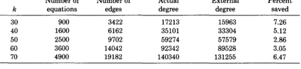
g, hj at this stage will result in a new clique {a, b, c] of size three.

In practical terms there is little additional cost involved in using external degree instead of true degree in the implementation (provided the number of indistinguishable nodes for each node is maintained). For the author’s program code it involves the addition of one line in the source program. In order to demonstrate that this modification can have savings in terms of fills, we tabulate runs on the k-by-k grid problem (nine-point difference operator) with varying values of k (see Table I).

It can be observed that there is a saving of from 3 percent to 7 percent of the number of nonzeros in the factored matrix by using external degree. Experiments have been performed on other less regular problems, and similar savings have been obtained. The saving is not dramatic; however, it is obtained with virtually

(8)

Table I. Number of Off-Diagonal Nonzeros in the Matrix Factors Using Actual and External Degree on the k-by-k Regular Grid Problem

Number of Number of Actual External Percent

k equations edges degree degree saved

30 900 3422 17213 15963 7.26

40 1600 6162 35101 33304 5.12

50 2500 9702 59274 57579 2.86

60 3600 14042 92342 89528 3.05

70 4900 19182 140340 131255 6.47

no extra effort. Furthermore, the saving in storage here implies a higher per- centage saving in arithmetic operations to perform the numerical factorization. 6. NUMERICAL EXPERIMENTS

The ordering algorithm as modified by multiple elimination (Section 4) and external degree (Section 5) has been implemented using standard FORTRAN. A parameter called DELTA is provided to the subroutine. If the value of DELTA is greater than or equal to zero, multiple elimination will be used in producing the ordering, and DELTA provides the tolerance factor as described in Section 4.2. If DELTA is -1, the subroutine will produce the conventional minimum- degree ordering (using external degree), that is, one degree update after each mass elimination. In the results tabulated in this section, we have labeled this the minimum-external-degree algorithm.

To demonstrate the improvement, we have included the result of GENQMD from the SPARSPAK [8] (that is, the minimum-degree ordering routine in the package). Note that the case when DELTA equals -1 is essentially the same as GENQMD, except that the incomplete-degree-update technique and external degree have been incorporated.

The runs from the minimum-degree routine of the Yale Sparse Matrix Package YSMP [4] are also included for comparison. It differs from GENQMD in the use of an incomplete-degree-update technique and the use of linked lists to represent elimination graphs.

All the experiments were run on a VAX 11/780, and the times reported in this section are in seconds on this machine.

6.1 Star Graph

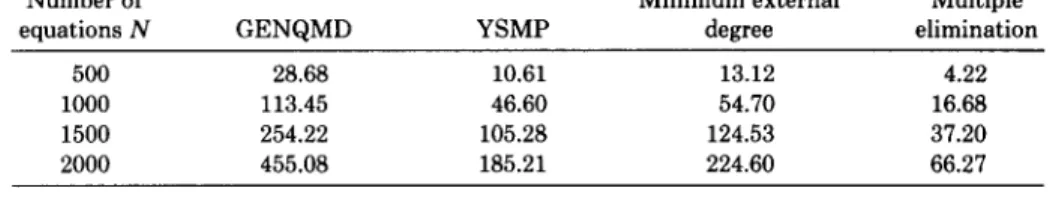
The different programs are used to order the star graph of N nodes, that is, a graph in which N - 1 nodes are connected to one center node. The graph structure, though simple, serves to demonstrate the effectiveness of the incomplete-degree-update strategy and the multiple-elimination scheme. Table II shows the time for the different methods.

All methods produce the best possible ordering for the star graph, that is, numbering the center node last or next to last. However, the time required to perform the task varies drastically among the methods. The method proposed in this paper runs about seven times faster than GENQMD and almost three times faster than YSMP. Admittedly, this is only a contrived example, but it does indicate the dramatic savings that are possible. In the Sections 6.2 and 6.3, significant savings are demonstrated on practical matrix examples.

(9)

Table II. Execution Time on the Star Graph of N Nodes Number of

equations N GENQMD YSMP

Minimum external degree Multiple elimination 500 28.68 10.61 13.12 4.22 1000 113.45 46.60 54.70 16.68 1500 254.22 105.28 124.53 37.20 2000 455.08 185.21 224.60 66.27

Table III. Execution Time on the k-by-k Grid

Multiple elimination:

Minimum external DELTA

k CENQMD YSMP degree 0 5

30 3.69 1.54 1.85 1.39 1.31

40 6.39 2.93 3.42 2.43 2.38

50 11.43 4.63 4.97 3.79 3.78

60 16.63 6.88 7.39 5.45 5.41

70 22.87 8.94 9.83 7.66 7.51

Table IV. Number of Off-Diagonal Nonzeros in Matrix Factor on the k-by-k Grid Multiple elimination:

k GENQMD YSMP degree 0 5

30 16633 17062 15836 15963 16924

40 36630 37322 33340 33304 33585

50 67773 61629 58660 57579 57946

60 101824 97886 90225 89528 89175

70 139979 137617 132719 131255 131377

6.2

k-by-k

Regular Grid

The different schemes were applied to the regular k-by-k grid, with k = 30, 40,

50,60,70. The nine-point difference operator is assumed. Table III compares the

execution time in seconds, while Table IV compares the quality of the resulting

orderings in terms of the number of off-diagonal nonzeros in the factor matrices.

The results in Table III show that the minimum-external-degree

algorithm

enjoys over 50 percent improvement in execution time over the GENQMD

version. This is mainly due to the incomplete-degree-update strategy. On the

other hand, the use of the multiple-elimination

technique (i.e., DELTA = 0)

reduces the execution time by about 25 percent over the minimum-external-

degree method (DELTA = -1).

Table IV compares the quality of the resulting orderings. The ordering pro-

duced by the modified version with multiple elimination (DELTA = 0) and

external degree is consistently the best or close to the best. This justifies the use

of these modifications. It is interesting to note from this table that there can be

a difference of over 15 percent in terms of the number of off-diagonal nonzeros

in the matrix factor between the best and the worst orderings, and they represent

orderings from basically the same algorithm.

(10)

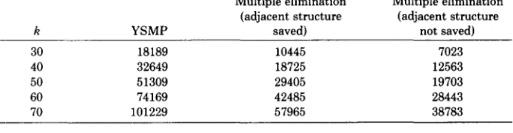
Table V. Minimal Storage Requirement (Number of Words) for Ordering on the k-by-k Grid Multiple elimination Multiple elimination

(adjacent structure (adjacent structure

k YSMP saved) not saved)

30 18189 10445 7023

40 32649 18725 12563

50 51309 29405 19703

60 74169 42485 28443

70 101229 57965 38783

Another point worth mentioning is that there is no apparent advantage in

using a positive DELTA for the

k-by-k

grid problem. Other values of DELTA

were tried, and similar results were obtained. The next section contains some

runs in which a positive DELTA produces noticeable reductions in ordering time.

The ordering routine from the Yale Sparse Matrix Package, YSMP, performs

quite well. It requires less time than the minimum-external-degree

method. It

uses more storage (in the form of linked lists) to represent the elimination graphs

and hence has a more efficient way of doing the elimination graph transformation.

Yet our modified version uses less execution time (from 10 to 20 percent),

requires significantly less core storage, and produces a marginally better ordering.

In Table V we tabulate the

minimal

amount of core storage required to execute

the ordering routine of YSMP and our version for the k-by-k grid problem. Here,

we have used half integers (INTEGER * 2) for indexing arrays whenever possible.

The YSMP ordering routine requires more than two and a half times the storage,

since it duplicates the adjacency structure in the form of linked lists, and full

integers (INTEGER * 4) have to be used for the linked values.

On the other hand, our version performs the ordering “in-place” within the

given adjacency structure. This will of course destroy the original matrix struc-

ture. The storage requirement for ordering can have an important bearing on the

solution of very large sparse problems where the ordering is performed in-core

and numerical factorization and solution are done out of core.

6.3 Harwell-Boeing Sparse Matrix Test Problems

Selected problems from the Harwell-Boeing collection of sparse matrix examples

[2] were tested using the different ordering schemes, in order to demonstrate the

performance of the modified version of the minimum-degree algorithm on a

variety of practical problems. Table VI contains the list of problem examples

selected, and we use the same keys as provided by the Harwell-Boeing tape to

identify the different matrices.

Nine symmetric and three unsymmetric matrices are used. For the unsymme-

tric examples, we use the structure

A + A

T. Table VII compares the execution

time of the different schemes, while Table VIII compares their fill-reducing

performances.

The results tabulated in Tables VII and VIII provide observations similar to

those for the

k-by-k

regular grid problem. The modified version runs more than

seven times faster than GENQMD for the problem “FS 451 1” and more than

(11)

Table VI. Selected Harwell-Boeine Test Matrices

Key Number of equations BCSPWROS 1723 BCSPWRlO 5300 BCSSTKOB 1074 BCSSTK13 2003 BCSSTMl3 2003 BLCKHOLE 2132 CAN 1072 1072 DWT 2680 2680 LSHP3466 3466 Description

Symmetric structure of western US power network Symmetric structure of entire US power network Symmetric stiffness matrix, frame building (TV studio) Symmetric stiffness matrix, fluid flow gen. eigenvalues Symmetric mass matrix, fluid flow gen. eigenvalues Connectivity struct of a geodesic dome on a coarse base Symmetric pattern from Cannes, Lucien Marro Symmetric connection table from DTNSRDC, Washington

Symmetrix matrix from Alan George’s L-SHAPE problems

FS 541 1 541

SHL 400 663

BP 1600 822

Unsymmetric facsimile convergence matrix Unsymmetric basis from LP problem SHELL Unsymmetric basis from LP problem BP

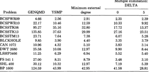
Table VII. Execution Time on Harwell-Boeing Examples

Problem GENQMD YSMP degree 0 5

BCSPWROS 4.66 2.56 2.91 2.35 2.39 BCSPWRlO 22.17 10.46 12.59 10.33 9.92 BCSSTK08 95.27 35.16 32.80 17.72 13.37 BCSSTK13 135.85 37.63 29.99 27.16 23.51 BCSSTM13 23.71 7.64 7.38 6.07 5.28 BLCKHOLE 9.85 3.90 4.40 3.35 3.79 CAN 1072 10.96 4.32 5.10 3.83 3.14 DWT 2680 25.58 10.08 12.97 9.90 8.44 LSHP3466 11.25 6.29 6.94 5.52 5.40 FS 541 1 27.00 8.21 8.79 3.48 3.10 SHL 400 30.12 10.32 12.97 7.19 5.39 BP 1600 124.59 43.99 42.95 41.58 28.81

five times faster for the problem BCSSTK08. For these two problems the YSMP ordering routine requires more than twice the amount of ordering time. For the other problems the modified version generally requires less time for ordering, and the savings are often quite significant.

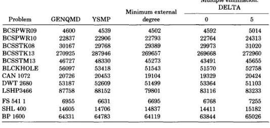
In terms of the quality of the ordering, the modified version produces either the best or close to the best ordering.

The modified version with DELTA = 5 generally requires the least amount of ordering time. The saving for the problem BP 1600 is quite substantial. However, the quality of the resulting ordering in terms of the number of off-diagonal nonzeros in the factor matrix is generally inferior to the others. Hence, the saving in ordering time will be more than offset by the increase in numerical factorization and solution time resulting from an inferior ordering. The use of a positive- tolerance-value DELTA is therefore not recommended.

(12)

152 l Joseph W. H. Liu

Table VIII. Number of Off-Diagonal Nonzeros in Matrix Factor on Hanvell-Boeing Examples

Problem

GENQMD YSMP degree 0 5

BCSPWROS 4600 4539 4502 4592 5014 BCSPWRlO 22837 22906 22793 22764 24313 BCSSTK08 30167 29768 29389 29973 31020 BCSSTK13 270925 287946 269657 269668 272960 BCSSTM13 46727 48330 45273 43491 45655 BLCKHOLE 56097 53418 51543 51570 52758 CAN 1072 20726 20453 19104 19329 20424 DWT 2680 53187 52609 51499 53364 51103 LSHP3466 87758 88152 79801 83116 83233 FS 541 1 6955 6631 6695 6768 SHL 400 14605 14706 14837 14411 BP 1600 64331 64783 64119 63844 7255 15182 7. CONCLUDING REMARKS

In this paper we have modified the conventional minimum-degree algorithm by introducing the notions of multiple elimination and external degree. This has resulted in a different but closely related ordering algorithm. Our experimental results indicate that the modified version consistently retains the fill-reducing property of the ordering scheme and often produces the best ordering in terms of fills among its competitors. Moreover, it can be implemented to run faster than the original approach. The saving in ordering time is problem-dependent. For some problems the modified algorithm runs a few times faster than existing implementations of the minimum-degree algorithm.

The reduction in ordering time can be explained as follows. The modification to the algorithm contributes to earlier detections of indistinguishable nodes and outmatched nodes. More important, it helps to reduce the number of degree updates necessary to effect the minimum-degree selection.

If we apply the modified algorithm to the k-by-k regular grid, the result corresponds quite closely to the nested dissection ordering specified in a “bottom- up” manner. This helps to explain the till-reducing property of the algorithm.

REFERENCES

1. DUFF, IS. A sparse future. In Sparse Matrices and Their Uses, I.S. Duff, Ed. Academic Press, New York, 1982, pp. l-29.

2. DUFF, I.S., GRIMES, R., LEWIS, J., AND POOLE, B. Sparse matrix test problems. SIGNUM Newsletter (June 1982), 22.

3. DUFF, I.S., AND REID, J.K. The multifrontal solution of indefinite sparse symmetric linear systems. ACM Trans. Math Softw. 9,3 (Sept. 1983), 302-325.

4. EISENSTAT, S.C., GURSKY, M.C., SCHULTZ, M.H., AND SHERMAN, A.H. The Yale Sparse Matrix Package, I. The symmetric code. Res. Rep. 112, Dept. of Computer Science, Yale Univ., New Haven, Conn., 1977.

5. EISENSTAT, S.C., SCHULTZ, M.H., AND SHERMAN, A.H. Applications of an element model for Gaussian elimination. In Sparse Matrix Computations, J.R. Bunch and D.J. Rose, Eds. Academic Press, New York, 1976 pp. 85-96.

(13)

6. GEORGE, A., AND LIU, J.W.H. A fast implementation of the minimum degree algorithm using quotient graphs. ACM Trans. Math Softw. 6,3 (Sept. 1980), 337-358.

7. GEORGE, J.A., AND LIU, J.W.H. Computer Solution of Large Sparse Positive Definite Systems. Prentice-Hall, Englewood Cliffs, N.J., 1981.

8. GEORGE, J.A., LIU, J.W.H., AND NG, E. User guide for SPARSPAK, Waterloo Sparse Linear Equations Package. Res. Rep. CS 78-30 (revised 1980), Dept. of Computer Science, Univ. of Waterloo, Waterloo, Ont., Can., 1980.

9. PETERS, F.J. Parallel pivoting algorithms for sparse symmetric matrices. Tech. Rep., Dept. of Mathematics and Computer Science, Eindhoven Univ. of Technology, Eindhoven, Neth., 1982. 10. ROSE, D.J. A graph-theoretic study of the numerical solution of sparse positive definite systems

of linear equations. In Graph Theory and Computing, R.C. Read, Ed. Academic Press, New York, 1973, pp. 183-217.

11. TINNEY, W.F., AND WALKER, J.W. Direct solution of sparse network equations by optimally ordered triangular factorization. Proc. IEEE 55 (1967), 1801-1809.

12. YANNAKAKIS, M. Computing the minimum fill-in is NP-complete. SIAM J. Alg. Disc. Meth. 1 (1981), 77-79.