SILVar: Single Index Latent Variable Models
Jonathan Mei and Jos´e M.F. Moura
Abstract—A semi-parametric, non-linear regression model in the presence of latent variables is introduced. These latent vari-ables can correspond to unmodeled phenomena or unmeasured agents in a complex networked system. This new formulation allows joint estimation of certain non-linearities in the system, the direct interactions between measured variables, and the effects of unmodeled elements on the observed system. The particular form of the model is justified, and learning is posed as a regularized maximum likelihood estimation. This leads to classes of structured convex optimization problems with a “sparse plus low-rank” flavor. Relations between the proposed model and several common model paradigms, such as those of Robust Principal Component Analysis (PCA) and Vector Autoregression (VAR), are established. Particularly in the VAR setting, the low-rank contributions can come from broad trends exhibited in the time series. Details of the algorithm for learning the model are presented. Experiments demonstrate the performance of the model and the estimation algorithm on simulated and real data.
I. INTRODUCTION
How real is this relationship? This is a ubiquitous ques-tion that presents itself not only in judging interpersonal connections but also in evaluating correlations and causality throughout science and engineering. Two reasons for reaching incorrect conclusions based on observed relationships in col-lected data are chance and outside influences. For example, we can flip two coins that both show heads, or observe that today’s temperature measurements on the west coast of the continental USA seem to correlate with tomorrow’s on the east coast throughout the year. In the first case, we might not immediately conclude that coins are related, since the number of flips we observe is not very large relative to the possible variance of the process, and the apparent link we observed is up to chance. In the second case, we still may hesitate to use west coast weather to understand and predict east coast weather, since in reality both are closely following a seasonal trend.
Establishing interpretable relationships between entities while mitigating the effects of chance can be achieved via sparse optimization methods, such as regression (Lasso) [1] and inverse covariance estimation [2]. In addition, the exten-sion to time series via vector autoregresexten-sion [3], [4] yields interpretations related to Granger causality [5]. In each of these settings, estimated nonzero values correspond to actual relations, while zeros correspond to absence of relations.
However, we are often unable to collect data to observe all relevant variables, and this leads to observing relationships that may be caused by common links with those unobserved variables. The hidden variables in this model are fairly general; they can possibly model underlying trends in the data, or This work partially funded by NSF grants CCF 1011903 and CCF 1513936.
the effects of a larger network on an observed subnetwork. For example, one year of daily temperature measurements across a country could be related through a graph based on geographical and meteorological features, but all exhibit the same significant trend due to the changing seasons. We have no single sensor that directly measures this trend. In the literature, a standard pipeline is to de-trend the data as a preprocessing step, and then estimate or use a graph to describe the variations of the data on top of the underlying trends [6]–[8].
Alternatively, attempts have been made to capture the effects of hidden variables via sparse plus low-rank optimization [9]. This has been extended to time series [10], and even to a non-linear setting via Generalized Linear Models (GLMs) [11]. What if the form of the non-linearity (link function) is not known? Regression using a GLM with an unknown link function is also known as a Single Index Model (SIM). Recent results have shown good performance when using SIMs for sparse regression [12].
So far, when choosing a model, current methods will impose a fixed form for the (non-)linearity, assume the absence of any underlying trends, perform separate pre-processing or partitioning in an attempt to remove or otherwise explicitly handle such trends, or take some combination of these steps. To address all of these issues, we propose a model with a non-linear function applied to a linear argument that captures the effects of latent variables, which manifest as unmodeled trends in the data. Thus, we introduce the Single Index Latent Variable (SILVar) model, which uses the SIM in a sparse plus low-rank optimization setting to enable general, interpretable multi-task regression in the presence of unknown non-linearities and unobserved variables. That is, we propose the SILVar model not only to use for regression in difficult settings, but also as a tool for uncovering hidden relationships buried in data.
First, we establish notation and review prerequisites in Section II. Next, we introduce the SILVar model and discuss several paradigms in which it can be applied in Section III. Then, we detail the numerical procedure for learning the SILVar model in Section IV. Finally, we demonstrate the performance via experiments on synthetic and real data in Section V.
II. BACKGROUND
In this section, we introduce the background concepts and notation used throughout the remainder of the paper.
A. Bregman Divergence and Convex Conjugates
For a given convex functionφ, the Bregman Divergence [13] associated withφ betweenyandxis denoted
Dφ(ykx) =φ(y)−φ(x)− ∇φ(x)>(y−x). (1)
The Bregman Divergence is a non-negative (asymmetric) quasi-metric. Two familiar special cases of the Bregman Divergence are Euclidean Distance when φ(x) = 12kxk2
2 and Kullback-Liebler Divergence whenφ(x) =P
i
xilogxi in the
case that x is a valid probability distribution (i.e.,x≥0and
P
i
xi= 1).
The convex conjugateφ∗ of a function φis given by
φ∗(x)
∆
= sup
y
y>x−φ(y). (2) The convex conjugate arises naturally in optimization prob-lems when deriving a dual form for the original (primal) problem. For closed, convex, differentiable, invertible 1-D functionφ, the following properties hold
φ∗(x) =x(∇φ)−1(x)−φ((∇φ)−1(x)) (∇φ)−1=∇φ∗ (φ∗)∗=φ
(3) where(·)−1denotes the inverse function, not the multiplicative inverse. In words, these properties give an alternate form of the conjugate in terms of gradients of the original function, state that the function inverse of the gradient is equal to the gradient of the conjugate, and state that the conjugate of the conjugate is the original function.
The first property can be seen by differentiating the expres-sion in the definition of the conjugate (2) with respect to y to determine the maximizing argument y and plugging it into the expression,
x− ∇φ(y) = 0⇒y= (∇φ)−1(x)
⇒φ∗(x) =x(∇φ)−1(x)−φ((∇φ)−1(x))
(4) The second property can be inferred by further differentiating expression (4), ∇φ∗(x) = (∇φ)−1(x) +x∇ (∇φ)−1(x) − ∇φ (∇φ)−1(x) ∇ (∇φ)−1(x) = (∇φ)−1(x). (5)
The third property can be shown by applying the first and second properties twice,
(φ∗)∗(x) =x∇φ(x)−φ∗(∇φ(x)) (a) = x∇φ(x)− ∇φ(x)(∇φ)−1(∇φ(x))− φ (∇φ)−1(∇φ(x)) =x∇φ(x)− ∇φ(x)x+φ(x) =φ(x), (6)
where(a)comes from applying the first property again on the second term.
B. Generalized Linear and Single-Index Models
The Generalized Linear Model (GLM) can be described using several parameterizations. We adopt the one based on the Bregman Divergence [14]. For observations yi ∈ R and
xi ∈Rp, lety = (y1. . . yn)>,X = (x1. . .xn). The model is parameterized by 1) a non-linear link functiong= (∇φ)−1
whereφis a closed, convex, differentiable, invertible function; and 2) a vector a∈Rp. We have the model written as
E[yi|xi] =g a>xi, (7)
(note that some references useg−1 as the link function where we use g) and the corresponding likelihood function written as
P(yi|xi) = exp
−Dφ yikg a>xi (8)
where the likelihood is expressed with respect to an appro-priate base measure [15], which can be omitted for notational clarity.
Let G = φ∗ and g = ∇G = (∇φ)−1. Then, for data
{xi, yi} with conditionally independentyigivenxi (note that
this is not necessarily assuming that xi are independent), learning the model a assuming g is known can be achieved via the Maximum Likelihood Estimator (MLE),
b a= argmax a n Y i=1 exp −Dφ yikg a>xi = argmin a n X i=1 Dφ yikg a>xi = argmin a n X i=1 φ(yi)−φ g a>xi −∇φ g a>xi yi−g a>xi (a) = argmin a n X i=1 G∗(yi)−yi a>xi −φ g a>xi + a>xig a>xi (b) = argmin a n X i=1 G∗(yi) +G a>xi−yi a>xi = argmin a b F1(y,X, g,a) (9) where equality (a) arises from the second property in (3), equality(b)arises from the first property, and we introduce
b F1(y,X, g,a)=∆ 1 n n X i=1 h G∗(yi) +G a>xi −yi a>xi i (10)
for notational compactness.
The Single Index Model (SIM) [16] takes the same form as the GLM. The crucial difference is in the estimation of the models. When learning a GLM, the link functiong is known and the linear parameterais estimated; however when learning a SIM, the link function g needs to be estimated along with the linear parameter a.
Recently, it has been shown that, when the function g is restricted to be monotonic increasing and Lipschitz, learning SIMs becomes computationally tractable [15] with perfor-mance guarantees in high-dimensional settings [12]. Thus, with scalar u defining the set Cu = {g : ∀y > x, 0 ≤
g(y)−g(x)≤u(y−x)}of monotonic increasingu-Lipschitz functions, this leads to the optimization problem,
(bg,ba) = argmin g,a b F1(y,X, g,a) s.t. g=∇G∈ C1. (11)
C. Lipschitz Monotonic Regression and Estimating SIMs
The estimation of g with the objective function includ-ing terms G and G∗ at first appears to be an intractably
difficult calculus of variations problem. However, there is a marginalization technique that cleverly avoids directly esti-mating functional gradients with respect to G and G∗ [15]
and admits gradient-based optimization algorithms for learn-ing. The marginalization utilizes Lipschitz monotonic regres-sion (LMR) as a subproblem. Thus, before introducing this marginalization, we first review LMR.
1) LMR: Given ordered pairs {xi, yi} and independent
Gaussianwi, consider the model
yi=g(xi) +wi, (12)
which intuitively treats {yi} as noisy observations of a
func-tion g indexed by x, sampled at points{xi}. Letegi =g(xi),
an estimate of the function value, with eg= (eg1. . .egn)
>, and
x[j] denote the jth element of the {xi} sorted in ascending
order. Then LMR is described by the problem,
e g∆=LMR(y,x) = argmin g n X i=1 (g(xi)−yi)2 s.t.0≤g x[j+1] −g x[j] ≤x[j+1]−x[j] fori= 1, . . . , n−1. (13)
While there may be in fact infinitely many possible (contin-uous) monotonic increasing Lipschitz functions g that pass through the points eg, the solution vector ge is unique. We will introduce a simple yet effective algorithm for solving this problem later in Section IV-A.
2) Estimating SIMs: We now return to the objective
func-tion (11). Let eg=LMR(y,X>a). Then the gradient w.r.t. a
can be expressed in terms of an estimate ofgwithout explicit computation of Gor G∗, ∇aF1= n X i=1 [(egi−yi)xi]. (14)
This allows us to apply gradient or quasi-Newton methods to solve the minimization ina, which is itself a convex problem since the original problem was jointly convex ing anda.
III. SINGLEINDEXLATENTVARIABLEMODELS In this section, we build the Single Index Latent Variable (SILVar) model from fundamental concepts.
A. Multitask regression and latent variables
First, we extend the SIM to the multivariate case and then examine how latent variables can affect learning of the linear parameter. Let yi = (y1i . . . ymi)>, g(x) = (g1(x1) . . . gm(xm)) > , and A = (a1 . . . am) > . Consider the vectorization, E[yji|xi] =gj a>jxi ⇒E[yi|xi] =g(Axi). (15) For the remainder of this paper, we make an assumption that all gj=g for notational simplicity, though the same analysis
readily extends to the case where gj are distinct.
Now, let us introduce a set of latent variables zi ∈ Rr with r p and the corresponding linear parameter B = (b1. . .bm)>∈Rm×r(note we can incorporate a linear offset by augmenting the variable z ← (z> 1)> and adding the linear offset as a column ofB). This leads to the asymptotic maximum likelihood estimate,
g,A,B= argmin g,A,B F2(yi,xi,zi, g,A,B) s.t. g=∇G∈ C1, (16) where F2(yi,xi,zi, g,A,B) ∆ =E "m X j=1 h G∗(yj) +G(a > jxi+b > jzi) i −y>(Axi+Bzi) # . (17)
Now consider the case in which the true distribution remains the same, but we only observexi and not zi,
(bg,Ab) =argmin g,A F3(yi,xi, g,A) ∆ =E "m X j=1 h G∗(yji) +G(a > jxi) i s.t.g=∇G∈ C1 − y>i (Axi) # . (18)
We now propose a relation between the two models in (16) and (18), which will finally lead to the SILVar model. Here we present the abridged theorem, and relegate the full expressions and derivation to Appendix A. To establish notation, let primes ( 0) denote derivatives, hats (b) denote a parameter estimate with only observed variables, and overbars ( ) denote an underlying parameter estimate when we have access to both observed and latent variables.
Theorem 1. Assume that bg0(0) 6= 0 and that |bg00| ≤J and
|g00| ≤ J for some J ≤ ∞. Then, the parameters
b
A and A
from models(17)and (18) are related as
b
A≈q(A+L), (19)
whereq=g0(0)
b
g0(0) and rank(L)≤r+ 1.
Here, we give a more intuitive version of the theorem and a proof outline. The more precise version of the theorem and its proof are given in Appendix A.
Proof Outline. Starting by loosely following the analysis
in [11], we take the gradient of F2 (from (17)) w.r.t. A,B at(g,A,B), ∇ ABF2=E g Axi+Bzi −yi x>i z > i =0. (20)
Again taking the gradient ofF3(from (18)) w.r.t.Aat(bg,A)b ,
∇AF3=E h b g(Axi)b −yi x>i i =0. (21)
Combining the first term of (20) corresponding toAwith (21), E
h
g(Axi+Bzi)−g(b Axi)b
Then assuming that bg0(0) 6= 0, we use a first order Taylor series approximation at 0, E h g(0) +g0(0)(Axi+Bzi)−bg(0)−bg 0 (0)Axb i x>i i ≈0 ⇒Ab ≈qA+q BE[zix > i ] + (g(0)−bg(0))µ > x E[xix > i] † ≈q(A+L), (23)
whereµx=E[xi], andA† denotes the pseudoinverse of ma-trixA. Then, since rank B≤r, we see that rank L≤r+1
as it was to be shown. Note that we choose the point 0 for convenience; we can instead choose other points as long asbg0 is not0 everywhere, or, in words, the expectation ofyigiven
xi has nontrivial dependence onxi in the first place. Though the theorem poses a hard constraint on |gb00|, we hypothesize that this is a rather strong condition that can be weakened to be in line with similar models. Thus, we propose the SILVar model,
b
y=bgAb +Lb
x, (24)
and learn it using the optimization problem,
(bg,Ab,L) =argminb g,A,L b F3(Y,X, g,A+L) +h1(A) +h2(L) s.t.g=∇G∈ C1, (25) where b F3(Y,X, g,A)=1 n n X i=1 "m X j=1 h G∗(yji)+G a>jxi i −y>i(Axi) # , (26)
the empirical version ofF3, andh1andh2are regularizers on
A andL respectively. Two natural choices forh2 would be h2(L) = λ2kLk∗ the nuclear norm and h2(L) = I{kLk∗ ≤
λ2} the indicator of the nuclear norm ball, both relating to the nuclear norm of L, since L is approximately low rank due to the influence of a relatively small number of latent variables. We may choose different forms for h1 depending on our assumptions about the structure ofA. For example, if
Ais assumed sparse, we may useh1(A) =λ1kv(A)k1, the`1 norm applied element-wise to the vectorizedAmatrix. These examples are extensions to the “sparse and low-rank” models, which have been shown under certain geometric incoherence conditions to be identifiable [9]. In other words, if the sparse component is not too low-rank, and if the low-rank component is not too sparse, then AandLcan be recovered uniquely.
B. Connection to Related Problems
In this section, we show how the SILVar model can be used in various problem settings commonly considered throughout the literature.
1) Generalized Robust PCA: Though we posed our initial
problem as a regression problem, if we take our measurement vectors to bexi=ei the canonical basis vectors (i.e., so that the overall data matrix X=I), then we arrive at
b
Y=g(b Ab +L)b . (27)
This is precisely the model behind Generalized Robust PCA [17], but with the twist of estimating the link function
as well [18]. What is worth noting is that although we arrived at our model via a regression problem with latent variables, the model itself is also able to describe a problem that arises from very different assumptions on how the data is generated and structured.
We also note that the SILVar model can be modified to share a space with the Generalized Low-Rank (GLR) Models [19]. The GLR framework is able to describe arbitrary types of data with an appropriate choice of convex link function g determined a priori, while the SILVar model is restricted to a certain continuous class of convex link functions but aims to learn this function. The modification is simply a matrix factorization L = UV (and “infinite” penalization on A). The explicit factorization makes the problem non-convex but instead block convex, which still allows for alternating convex steps in U with fixed V (and vice versa) to tractably reach local minima under certain conditions. Nonetheless, due to the non-convexity, further discussion of this particular extension will be beyond the scope of this paper.
2) Extension to Autoregressive Models: We can apply the
SILVar model to learn from time series as well. Consider a set of N time series each of length K, X ∈ RN×K. We assume the noise at each time step is independent (note that, with this assumption, the time series are still dependent across time), and take in our previous formation,yi←xk andxi ← xk−1:k−M = (x>k−1. . .x
>
k−M)> so that the model of order
M takes the form,
b xk =g M X i=1 A(i)+L(i)xk−i ! , (28) and learn it using the optimization problem,
(bg,Ab,Lb) = argmin g,A,L b F4(X, g,A+L) +h1(A) +h2(L) s.t.g=∇G∈ C1, (29) whereA= A(1). . .A(M) andL= L(1). . .L(M) and b F4(X, g,A) = 1 K−M K X k=M+1 "N X j=1 " G∗(xjk)+G M X i=1 a(ji)xk−i !# −x>k M X i=1 A(i)xk−i !# , where A(i) = a1(i). . .a(Ni) >
, similarly to before. Note that the analysis in the previous section follows naturally in this setting, so that here rank(Li) ≤ r+ 1. Then, the matrix A may be assumed to be group sparse, relating to generalized notions of Granger Causality [3], [20], and one possible corresponding choice of regularizer taking the form h1(A) =λ1P i,j a(1)ij . . . a(ijM) 2.
Another structural assumption could be that of the Causal Graph Process model [21], inspired by Signal Processing on Graphs [6], in which A(i) are matrix polynomials in one underlying matrix Ae. This framework utilizes the nonconvex
regularizer h1(A) = λ1kv(A(1))k1 + λ2P
i6=j
kA(i)A(j) −
A(j)A(i)k2
F to encourage both sparsity and commutativity,
same matrix. Since this particular regularization is again block convex, convex steps can still be taken in each A(i) with all other blocks A(j) for j 6= i fixed, for a computationally tractable algorithm to reach a local minimum under certain conditions. However, further detailed discussion will remain outside the scope of this paper.
The hidden variables in this time series model can even possibly model underlying trends in the data. For example, one year of daily temperature measurements across a country could be related through a graph based on geographical and meteorological features, but all exhibit the same significant trend due to the changing seasons. In previous work, a standard pipeline is to detrend the data as a preprocessing step, and then estimate or use a graph to describe the variations of the data on top of the underlying trends [6]–[8]. Instead, the time series can also be modeled as a modified autoregressive process, depending on a low-rank trend L0 = `0
1 . . . `
0 K
∈ RN×K and the variations of the process about that trend,
b xk =g M X i=1 A(i)+L(i)xk−i ! =g `0k+ M X i=1 A(i) xk−i−`0k−i ! ⇒ M X i=1 L(i)xk−i=`0k− M X i=1 A(i)`0k−i (30)
Thus we estimate the trend using ridge regression for numer-ical stability purposes but without enforcing L0 is low rank. We can accomplish this via the simple optimization,
b L0= argmin L0 K X k=M+1 `0k− M X i=1 A(i)`0k−i− M X i=1 L(i)xk−i 2 2 +λkL0k2 F (31)
with λ being the regularization parameter. In this way, the extension of SILVar to autoregressive models can allow joint estimation of the effects of the trend and of these variations supported on the graph, as will be demonstrated via experi-ments in Section V.
IV. EFFICIENTLYLEARNINGSILVARMODELS In this section, we describe the formulation and correspond-ing algorithm for learncorrespond-ing the SILVar model. Surpriscorrespond-ingly, in the single-task setting, learning a SIM is jointly convex in g andaas demonstrated in [15]. The pseudo-likelihood function
b
F3 used for learning the SILVar model in (29) can be shown to be jointly convex in g,A, andL by an extension from the single-task regression setting.
Lemma 2 (Corollary of Theorem 2 of [15]). The Fb3 in the
SILVar model learning problem(24)is jointly convex ing,A,
and L.
This convexity is enough to ensure that the learning can converge and be computationally efficient. Before describing the full algorithm, one detail remains: the implementation of the LMR introduced in Section II-C.
A. Lipschitz Monotonic Regression
To tackle LMR, we first introduce the related simpler problem of monotonic regression, which is solved by a well-known algorithm, the pooled adjacent violators (PAV) [22]. The monotonic regression problem is formulated,
PAV(y,x)= argmin∆ g n X i=1 (g(xi)−yi) 2 s.t. 0≤g x[j+1] −g x[j] . (32)
The PAV algorithm has a complexity of O(n), which is due to a single complete sweep of the vectory.
We introduce a simple generalization to the monotonic regression, GPAVt(y,x) ∆ = argmin g n X i=1 (g(xi)−yi) 2 s.t. t[j+1]≤g x[j+1] −g x[j] for j= 1, . . . , n−1. (33)
This modification allows weaker (if ti < 0) or stronger (if
ti > 0) local monotonicity conditions to be placed on the
estimated function g. Let t[1] = 0 and s[i] =
i
P
j=1
t[j], and rewriting in vectorized form,
s=∆cusum(t). (34)
Then, we can rewrite,
GPAVt(y,x) = argmin g n X i=1 (g(xi)−si−(yi−si))2 s.t.0≤g x[j+1] −s[j+1]− g x[j] −s[j] forj= 1, . . . , n−1, (35)
which leads us to recognize that
GPAVt(y,x) =PAV(y−s,x) +s. (36) Then, returning to LMR (13), we can split the variable g
into its positive and negative parts,g+≈gandg−≈ −g, to
take advantage of the fast PAV algorithm,
LMR(y,x) = argmin g+,g− n X i=1 1 2(g+(xi)−yi) 2 +1 2(g−(xi)−(−yi)) 2 s.t.0≤g+ x[j+1] −g+ x[j] x[j]−x[j+1]≤g− x[j+1] −g− x[j] forj= 1, . . . , n−1 g++g−= 0. (37)
Then forming the augmented Lagrangian with dual variable
w, LMR(y,x) = argmin g+,g− n X i=1 1 2(g+(xi)−yi) 2 +1 2(g−(xi) +yi) 2 +ρ 2kg++g−+wk 2 2− ρ 2kwk 2 2 s.t.0≤g+ x[i+1] −g+ x[i] x[i]−x[i+1]≤g− x[i+1] −g− x[i] fori= 1, . . . , n−1, (38)
Algorithm 1 Lipschitz monotone regression (LMR)
1: Let t1 = 0 and compute t[i+1] = x[i] −x[i+1], s = cusum(t). Set rateρ.
2: Initialize g+ = PAV(y,x), g− = PAV(−y−s,x) +s,
w=0 3: whilekg++g−k ≥ do 4: g+←PAV y−ρ(g −+w) 1+ρ ,x 5: g−←PAV −y−ρ(g ++w) 1+ρ −s,x +s 6: w←w+g++g− 7: end while 8: returng= (g+−g−)/2
we can use the augmented dual method of multipliers (ADMM) [23] to perform this optimization efficiently utilizing PAV as a subroutine. This is described in Algorithm 1.
While the GPAV allows us to quickly perform Lipschitz monotonic regression with our particular choice oft, it should be noted that using other choices for tcan easily generalize the problem to bi-H¨older regression as well, to find functions in the set Cu,β`,α ={g : ∀y > x, `|y−x|α ≤g(y)−g(x)≤
u|y−x|β}. This set may prove interesting for further analysis
of the estimator and is left as a topic for future investigation.
B. Optimization Algorithms
With LMR in hand, we can outline the algorithm for solving the convex problem (25). This procedure can be performed for general h1 andh2, but proximal mappings are efficient to compute for many common regularizers. Thus, we describe the basic algorithm using gradient-based proximal methods (e.g., accelerated gradient [24], and quasi-Newton [25]), which require the ability to compute a gradient and the proximal mapping.
In addition, we can compute the objective function value for purposes of backtracking [26], evaluating algorithm con-vergence, or computing error (e.g., for validation or testing purposes). While our optimization outputs an estimate of g, the objective function depends on the value of G and its conjugate G∗. Though we cannot necessarily determine Gor
G∗ uniquely sinceG+candGboth yieldgas a gradient for
anyc∈R, the value ofG(x) +G∗(y)is unique for a fixedg.
To see this, consider Ge=G+cfor some constant c. Then, e G(x) +Ge∗(y) =G(x) +c+ max z [zy−Ge(z)] =G(x) +c+ max z [zy−G(z)−c] =G(x) + max z [zy−G(z)] =G(x) +G∗(y) (39)
This allows us to compute the objective function by per-forming the cumulative numerical integral of bg on points v(Θ)(e.g.,G=cumtrapz(theta,ghat)in Matlab). Then, a discrete convex conjugation (also known as the discrete Legendre transform (DLT) [27]) computes G∗.
We did not notice significant differences in performance accuracy due to our implementation using quasi-Newton meth-ods and backtracking compared to an accelerated proximal
gradient method, possibly because both algorithms were run until convergence. Thus, we show only one set of results. How-ever, we note that the runtime was improved by implementing the quasi-Newton and backtracking method.
Algorithm 2 Single Index Latent Variable (SILVar) Learning
1: Initialize Ab =0,Lb =0
2: while not convergeddoProximal Methods
3: Computing gradients: Θ←(Ab +L)Xb e g←LMR(v(Y),v(Θ)) ∇AF3=∇LF3= X i∈I (bg(θi)−yi)x>i
4: Optionally compute function value:
b G←cumtrapz(v(Θ),bg) b G∗←DLT(v(Θ),Gb,v(Y)) b F3= X ij b G∗(yij) +G(b θij)−yijθij 5: end while 6: return (gb,A,L)
Algorithm 2 describes the learning procedure and details the main function and gradient computations while assuming a proximal operator is given. The computation of the gradient and the update vector depends on the particular variation of proximal method utilized; with stochastic gradients, the set I ⊂ {1, . . . , n} could be pseudorandomly generated at each iteration, while with standard gradients, I={1, . . . , n}. The cumtrapzprocedure takes as input the coordinates of points describing the functionbg. The DLT procedure takes as its first two inputs the coordinates of points describing the functionGb,
and as its third input the points at which to evaluate the convex conjugateGb∗.
Here, an observant reader may notice the subtle point that the functionG∗ may only be defined inside a finite or
semi-infinite interval. This can occur if the function g is bounded below and/or above, so that G has a minimum/maximum slope, and G∗ is infinite for any values below that minimum
or above that maximum slope of G (to see this, one may refer back to the definition of conjugation (2)). Fortunately, this does not invalidate our method. It is straightforward to see that gb(x) = x is always a feasible solution and that
b
G∗(y) = y2/2 is defined for all y; thus starting from this
solution, with appropriately chosen step sizes, gradient-based algorithms will avoid the solutions that make the objective function infinite. Furthermore, even if new datayjfalls outside the valid domain for the learnedGb∗and we incur an “infinite”
loss using the model, evaluatinggbAb +Bb
xjis still well defined. This problem is not unique to SIM’s, as assuming a fixed link function g in a GLM can also incur infinite loss if new data does not conform to modeling assumptions implicit to the link function (e.g., the log-likelihood for a negativey
under a non-negative distribution), and making a prediction using the learned GLM is still well-defined. Practically, the
loss for SILVar computed using the DLT may be large, but will not be infinite [27].
V. EXPERIMENTS
We study the performance of the algorithm via simulations on synthetically generated data as well as real data. In these experiments, we show the different regression settings, as discussed in Section III-B, under which the SILVar model can be applied.
A. Synthetic Data
The synthetic data corresponds to a multi-task regression setting. The data was generated by first creating random sparse matrix Af = (A Ah) where Ah ∈ Rp×H and H = bhpc the number of hidden variables, and h is the proportion of hidden variables. The elements of Af were first generated as i.i.d. Normal variables, and then a sparse mask was applied to choose bmlog10(p+H)cnon-zeros. Next, the data Xf= (X>X>h)> were generated with each vector drawn i.i.d. from a multivariate Gaussian with mean 0 and covariance matrix
Σf ∈ R(p+H)×(p+H). This was achieved by creating Σ1f/2
by thresholding a matrix with diagonal entries of 1 and off-diagonal entries drawn form an i.i.d. uniform distribution in the interval [−0.5,0.5] to be greater than 0.35 in magnitude. Then Σ1f/2 was pre-multiplied with a matrix of i.i.d. Normal variables. Finally, we generated Y = g(AfXf) +W for 2 different link functions g1(x) = log(1 +ec1x) and g2(x) =
2
1+e−c2x−1, andWis added i.i.d. Gaussian noise. Then, the
task is to learn (g,b Ab,L)b the SILVar model (24) from(Y,X)
without access toXh. As comparison, we use an Oracle GLM model, in which the truegis given but the parameters(Aob ,Lo)b
still need to be learned. We note that while there is a slight mismatch between the true and assumed noise distributions, the task is nonetheless difficult, yet our estimation using the SILVar model can still exhibit good performance with respect to the Oracle.
The experiments were carried out across a range of problem sizes. The dimension of yi was fixed at m = 25. The dimension of the observed xi was set to p ∈ {25,50}, and the proportion of the dimension of hidden xh was set to h ∈ {0.1,0.2}. The number of data samples was varied in k ∈ {25,50,100,150,200}. Validation was performed using a set of samples generated independently but using the same Af and g, and using a grid of (λS, λL) ∈
10i/4
i∈ {−8,−7, . . . ,7,8}
2
. The whole process of data generation and model learning is repeated 10 times for each experimental condition. The average `1 errors and mean squared errors (MSEs) between the true A and the best estimatedAb (determined via validation) are shown in Figure 1.
The first row is the`1 errors and the second row is the MSEs for the various experimental conditions. The empirical results show that the SILVar model and learning algorithm lose out slightly on performance for estimating the link function gbut overall still match the Oracle fairly well in most cases. We also see several other intuitive behaviors for both the SILVar and Oracle models: as we increase the amount of data n, the performance increases, and as we increase the proportion of
50 100 150 200 Number of samples (n) 0.05 0.1 0.15 k bA− A k1 / ( m p ) ℓ1error inA g(x) = log(1 +ecx) h=0.2; p=25; SILVar h=0.2; p=25; oracle h=0.1; p=25; SILVar h=0.1; p=25; oracle h=0.2; p=50; SILVar h=0.2; p=50; oracle h=0.1; p=50; SILVar h=0.1; p=50; oracle
(a)`1 error inAforg1
50 100 150 200 Number of samples (n) 0.06 0.08 0.1 0.12 0.14 0.16 k bA− A k1 / ( m p ) ℓ1error inA g(x) = 2/(1 +e−cx)−1 h=0.2; p=25; SILVar h=0.2; p=25; oracle h=0.1; p=25; SILVar h=0.1; p=25; oracle h=0.2; p=50; SILVar h=0.2; p=50; oracle h=0.1; p=50; SILVar h=0.1; p=50; oracle (b)`1 error inAforg2 50 100 150 200 Number of samples (n) 0 0.02 0.04 0.06 0.08 0.1 k bA− A k 2/F ( m p ) MSE inA g(x) = log(1 +ecx) h=0.2; p=25; SILVar h=0.2; p=25; oracle h=0.1; p=25; SILVar h=0.1; p=25; oracle h=0.2; p=50; SILVar h=0.2; p=50; oracle h=0.1; p=50; SILVar h=0.1; p=50; oracle (c) MSE inAforg1 50 100 150 200 Number of samples (n) 0.05 0.1 0.15 k bA− A k 2/F ( m p ) MSE inA g(x) = 2/(1 +e−cx)−1 h=0.2; p=25; SILVar h=0.2; p=25; oracle h=0.1; p=25; SILVar h=0.1; p=25; oracle h=0.2; p=50; SILVar h=0.2; p=50; oracle h=0.1; p=50; SILVar h=0.1; p=50; oracle (d) MSE inAforg2
Fig. 1: Different errors for estimatingA in Toy Data
hidden variables (from h = 0.1 to h = 0.2), performance decreases. We also note that g2 seems to be somehow more difficult to estimate thang1, and additionally that the perfor-mance of the SILVar model w.r.t. the Oracle model is worse withg2 than with g1. This could have something to do with the 2 saturations ing2as opposed to the 1 ing1, corresponding in an intuitive sense to a more non-linear setting that contains more information needing to be captured while estimatingbg.
B. Temperature Data
In this setting, we wish to learn the graph capturing relations between the weather patterns at different cities. The data is a real world multivariate time series consisting of daily temperature measurements (in ◦F) for 365 consecutive days during the year2011taken at each of150different cities across the continental USA.
Previously, the analysis on this dataset has been performed by first fitting with a4th order polynomial and then estimating a sparse graph from an autoregressive model using a known link functiong(x) =xassuming Gaussian noise [8].
Here, we fit the time series using a 2nd order AR SILVar model (28) with regularizers for group sparsity h1(A) = λ1P i,j a(1)ij . . . a(ijM) 2 wherea (m)
ij is theij entry of matrix A(m), and nuclear norm h2(L) = λ2
M P i=1 L(i) ∗. We also
estimate the underlying trend using (31).
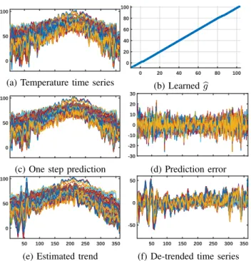
In Figure 2, we plot the original time series, estimated trends, the estimated network, and residuals. The plots are all from time steps 3 to 363, since those are the indices for the trends that we can reliably estimate using the simple procedure (31). In Figure 2a, we show the original time series, which clearly exhibit a seasonal trend winter–summer–winter. Figure 2b shows the estimated link function bg, which turns out to be linear, though a priori we might not intuitively expect a process as complicated as weather to behave this way when sampled so sparsely. Figures 2c and 2d show the full prediction xkb =
M
P
i=1
0 50 100
(a) Temperature time series
0 20 40 60 80 100 0 20 40 60 80 100 (b) Learnedbg 0 50 100
(c) One step prediction -30 -20 -10 0 10 20 30 (d) Prediction error 50 100 150 200 250 300 350 0 50 100
(e) Estimated trend
50 100 150 200 250 300 350
-50 0 50
(f) De-trended time series
Fig. 2: Time series, link function, trends, and prediction errors computed using the learned SILVar model
/RQ /DW
Fig. 3: Graph on weather stations learned using SILVar
xk−bxk, respectively. Figures 2e and 2f show the trend Lb
0
learned using (31) and the time series with the estimated trend removed, respectively. The trend estimation procedure captures the basic shape of the seasonal effects on the temperature. Several of the faster fluctuations in the beginning of the year are captured as well, suggesting that they were caused by some larger scale phenomena. Indeed there were several notable storm systems that affected the entire country in the beginning of the year in short succession [28], [29].
Figure 3 shows the network Ab0 that is estimated, where b a0ij = ba (1) ij . . .ba (M) ij
2. It is intuitively pleasing that the
patterns discovered match well previously established results based on first de-trending the data and then separately esti-mating a network [8]. That is, we see the effect of the Rocky Mountain chain around −110◦ to −105◦ longitude and the overall west-to-east direction of the weather patterns, matching the prevailing winds.
50 100 150 200 250 300 350 400 Number of Training Samples (n) 1.6 1.7 1.8 1.9 RMSE Prediction Errors GLM SILVar (a) -10 0 10 20 30 40 50 θ 0 10 20 30 40 50 b g ( θ )
Estimated link function
(b)
Fig. 4: (a) Root mean squared errors (RMSEs) from SILVar and Oracle models; (b) Link function learned using SILVar model
C. Bike Traffic Data
The bike traffic data was obtained from HealthyRide Pitts-burgh [30]. The dataset contains the timestamps and station locations of departure and arrival (among other information) for each of 127,559 trips taken between 50 stations within the city from May 31, 2015 to September 30, 2016, a total of 489 days.
We consider the task of using the total number of rides departing from and arriving in each location at 6:00AM-11:00AM to predict the number of rides departing from each location during the peak period of 11:00AM-2:00PM for each day. This corresponds to Y ∈ N500 ×489 and X ∈ N
100×489
0 ,
where N0 is the set of non-negative integers, and A,L ∈ R50×100. We estimate the SILVar model (24) and compare its performance against a sparse plus low-rank GLM model with an underlying Poisson distribution and fixed link function gGLM(x) = log(1 +ex). We use n ∈ {60,120,240,360}
training samples and compute errors on validation and test sets of size 48 each, and learn the model on a grid of
(λS, λL) ∈ 10i/4
i∈ {−8,−7, . . . ,11,12}
2
. We repeat this 10 times for each setting, using an independent set of training samples each time. We compute testing errors in these cases for the optimal(λS, λL)with lowest validation errors for
both SILVar and GLM models.
We also demonstrate that the low-rank component of the estimated SILVar model captures something intrinsic to the data. Naturally, we expect people’s behavior and thus traffic to be different on business days and on non-business days. A standard pre-processing step would be to segment the data along this line and learn two different models. However, as we use the full dataset to learn one single model, we hypothesize that the learned low-rank Lb captures some aspects of this
underlying behavior.
Figure 4a shows the test Root Mean Squared Errors (RM-SEs) for both SILVar and GLM models for varying training sample sizes, averaged across the 10 trials. We see that the SILVar model outperforms the GLM model by learning the link function in addition to the sparse and low-rank regression matrices. Figure 4b shows an example of the link function learned by the SILVar model withn= 360training samples. Note that the learned SILVar link function performs non-negative clipping of the output, which is consistent with the count-valued nature of the data.
We also test the hypothesis that the learned Lb contains
0 0.2 0.4 0.6 0.8 1 Detection Rate 0 0.2 0.4 0.6 0.8 1
False Alarm Rate
ROC for classifying business day
rank 1 rank 2 rank 3 rank 4 rank 5 rank 6 full
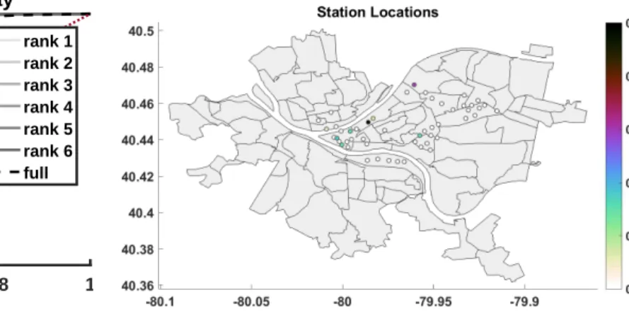
Fig. 5: Receiver operating characteristics (ROCs) for classify-ing each day as a business day or non-business day, usclassify-ing the low-rank embedding provided by Lb learned from the SILVar
model and using the full data
through its relatively low-dimensional effects on the data. We perform the singular value decomposition (SVD) on the optimally learned Lb =UbΣbVb> for n = 360 and project the
data onto the rtop singular components Xre =Σrb Vb>rX. We
then use Xre to train a linear support vector machine (SVM)
to classify each day as either a business day or a non-business day, and compare the performance of this lower dimensional feature to that of using the full vectorXto train a linear SVM. If our hypothesis is true then the performance of the classifier trained onXre should be competitive with that of the classifier
trained onX. We use 50 training samples ofXre and ofXand
test on the remainder of the data. We repeat this 50 times by drawing a new batch of 50 samples each time. We then vary the proportion of business to non-business days in the training sample to trace out a receiver operating characteristic (ROC). In Figure 5, we see the results of training linear SVM onXre
for r∈ {1, ...,6} and on the full data for classifying business and non-business days. We see that using only the first two singular vectors, the performance is fairly poor. However, by simply taking 3 or 4 singular vectors, the classification performance almost matches that of the full data. Surprisingly, using the top 5 or 6 singular vectors achieves performance greater than that of the full data. This suggests that the projection may even play the role of a de-noising filter in some sense. Since we understand that behavior should correlate well with the day being a business or a non-business, this competitive performance of the classification using the lower dimensional features strongly suggests that the low-rank Lb
indeed captures the effects of latent behavioral factors on the data.
Finally, in Figure 6, we plot the(i, i)entries of the optimal
b
A at n = 360. This corresponds to locations for which incoming bike rides at 6:00AM-11:00AM are good predictors of outgoing bike rides at 11:00AM-2:00PM, beyond the effect of latent factors such as day of the week. We may intuitively expect this to correlate with locations that have restaurants open for lunch service, so that people would be likely to ride in for lunch or ride out after lunch. This is confirmed by
Fig. 6: Intensities of the self-loop at each station
observing that these stations are in Downtown (-80,40.44), the Strip District (-79.975, 40.45), Lawrenceville (-79.96, 40.47), and Oakland (-79.96, 40.44). It is especially interesting to note that Oakland, sandwiched between University of Pittsburgh and Carnegie Mellon University, is included. Even though the target demographic is largely within walking distance, there is a high density of restaurants open for lunch, which may explain its non-zero coefficient. The remainder of the locations with non-zero coefficients aii are also near high densities
of lunch spots, while the other locations with coefficients aii of zero are largely either near more residential areas or
near restaurants more known for dinner or nightlife rather than lunch, such as Shadyside (x ≥ −79.95) and Southside (y≤40.43)).
VI. CONCLUSION
Data exhibit complex dependencies, and it is often a challenge to deal with non-linearities and unmodeled effects when attempting to uncover meaningful relationships among various interacting entities that generate the data. We intro-duce the SILVar model for performing semi-parametric sparse regression and estimating sparse graphs from data under the presence of non-linearities and latent factors or trends. The SILVar model estimates a non-linear link function g as well as structured regression matricesAandLin a sparse and low-rank fashion. We justify the form of the model and relate it to existing methods for general PCA, multi-task regression, and vector autoregression. We provide computationally tractable algorithms for learning the SILVar model and demonstrate its performance against existing regression models and methods on both simulated and real data sets, namely 2011 US weather sensor network data and 2015-2016 Pittsburgh bike traffic data. We see from the simulated data that the SILVar model matches the performance of an Oracle GLM that knows the true link function and only needs to estimateAandL; we show empiri-cally on the temperature data that the learnedLcan capture the effects of underlying trends in time series whileArepresents a graph consistent with US weather patterns; and we see that, in the bike data, SILVar outperforms a GLM with a fixed link function, the learned L encodes latent behavioral aspects of
the data, andAdiscovers notable locations consistent with the restaurant landscape of Pittsburgh.
APPENDIXA PROOF OFTHEOREM1
We first state a more precise version of the theorem.
Theorem 1. Assume that bg0(0) 6= 0 and that
|bg00| ≤ J and |g00| ≤ J for some J ≤ ∞.
Furthermore, assume in models (17) and (18)
that maxkAbkF,kAkF +kBkF ≤ QM N r and max Ekxik32 ,Ekxik2kzik22 ,Ekxik22kzik2 ≤ s3N r,
where the subscripts indicate that the bounds may grow with
the values in the subscript. Then, the parameters Ab and A
from models (17)and (18)are related as
b A≈q(A+L), where q= g0(0) b g0(0),µx=E[xi], and L= BE[zix>i ] + (g(0)−g(0))b µ > x E[xix>i ] † ⇒rank(L)≤r+ 1.
Then withE=∆Ab −q(A+L), we have
1 M NkEkF ≤ 2J σ` b g0(0)M√NQ 2 M N rs3N r.
The assumptions require that the 2nd order Taylor series expansion is accurate around the point 0, that the model pa-rameters are bounded, and that the distributions generating the data are not too spread out (beyond0where the Taylor series expansion is performed). These are all intuitively reasonable and unsurprising assumptions.
Now we give the proof of Theorem 1. We begin with the Taylor series expansion, using the Lagrange form of the remainder, E h b g(0) +gb 0 (0)Axb i−g(0)−g0(0)(Axi+Bzi) x>i i =E h b g00(ξ)(Axb i). ∧ 2−g00(η)(Axi+Bzi). ∧ 2x>i i , where |ξj| ≤ |bajxi|, |ηj| ≤ |ajxi+bjzi|, B = b1. . .bm >
similarly to before, x y denotes the element-wise (Hadamard) product, andx.∧2 =xxdenotes
element-wise squaring. Substituting the definitions of E and q, we have kEkF≤JE h (Axb i). ∧ 2+(Axi+Bzi). ∧ 2x>i F i b g0(0)E[xix > i] † F ≤J σ` √ N b g0(0) kAbk 2 F+kAk 2 F E[kxik32]+kBk 2 FE[kxik2kzik22] + 2kAkFkBkFE[kxik22kzik2] ,
where J is the bound on |bg00| ≤ J and |g00| ≤ J, σ ` = E xix>i †
2, the largest singular value of the
pseudo-inverse of the covariance. To finish off, we substitute the values given by the inequalities in our assumptions.
REFERENCES
[1] R. Tibshirani, “Regression Shrinkage and Selection via the Lasso,”
Journal of the Royal Statistical Society. Series B (Methodological), vol. 58, no. 1, pp. 267–288, 1996. [Online]. Available: http: //www.jstor.org/stable/2346178
[2] J. Friedman, T. Hastie, and R. Tibshirani, “Sparse inverse covariance estimation with the graphical Lasso,”Biostatistics, vol. 9, no. 3, pp. 432– 41, Jul. 2008. [Online]. Available: http://www.pubmedcentral.nih.gov/ articlerender.fcgi?artid=3019769&tool=pmcentrez&rendertype=abstract [3] A. Bolstad, B. Van Veen, and R. Nowak, “Causal network inference via
group sparse regularization,”IEEE Transactions on Signal Processing, vol. 59, no. 6, pp. 2628–2641, Jun. 2011.
[4] S. Basu and G. Michailidis, “Regularized estimation in sparse high-dimensional time series models,” The Annals of Statistics, vol. 43, no. 4, pp. 1535–1567, Aug. 2015. [Online]. Available: http://projecteuclid.org/euclid.aos/1434546214
[5] C. W. J. Granger, “Investigating causal relations by econometric models and cross-spectral methods,”Econometrica, vol. 37, no. 3, pp. 424–438, Aug. 1969. [Online]. Available: http://www.jstor.org/stable/1912791 [6] A. Sandryhaila and J. M. F. Moura, “Discrete Signal Processing on
Graphs,”IEEE Transactions on Signal Processing, vol. 61, no. 7, pp. 1644–1656, Apr. 2013.
[7] ——, “Discrete signal processing on graphs: Frequency analysis,”IEEE Transactions on Signal Processing, vol. 62, no. 12, pp. 3042–3054, Jun. 2014.
[8] J. Mei and J. M. F. Moura, “Signal Processing on Graphs: Causal Mod-eling of Unstructured Data,”IEEE Transactions on Signal Processing, vol. 65, no. 8, pp. 2077–2092, Apr. 2017.
[9] V. Chandrasekaran, P. A. Parrilo, and A. S. Willsky, “Latent variable graphical model selection via convex optimization,” The Annals of Statistics, vol. 40, no. 4, pp. 1935–1967, Aug. 2012. [Online]. Available: http://projecteuclid.org/euclid.aos/1351602527
[10] A. Jalali and S. Sanghavi, “Learning the Dependence Graph of Time Series with Latent Factors,” arXiv:1106.1887 [cs], Jun. 2011, arXiv: 1106.1887. [Online]. Available: http://arxiv.org/abs/1106.1887 [11] M. T. Bahadori, Y. Liu, and E. P. Xing, “Fast structure learning in
generalized stochastic processes with latent factors,” in Proceedings of the 19th ACM SIGKDD International Conference on Knowledge Discovery and Data Mining, ser. KDD ’13. New York, NY, USA: ACM, 2013, pp. 284–292. [Online]. Available: http://doi.acm.org/10. 1145/2487575.2487578
[12] R. Ganti, N. Rao, R. M. Willett, and R. Nowak, “Learning Single Index Models in High Dimensions,” arXiv:1506.08910 [cs, stat], Jun. 2015, arXiv: 1506.08910. [Online]. Available: http://arxiv.org/abs/1506.08910 [13] L. M. Bregman, “The relaxation method of finding the common point of convex sets and its application to the solution of problems in convex programming,” USSR Computational Mathematics and Mathematical Physics, vol. 7, no. 3, pp. 200–217, Jan. 1967. [Online]. Available: http://www.sciencedirect.com/science/article/pii/0041555367900407 [14] A. Banerjee, S. Merugu, I. S. Dhillon, and J. Ghosh, “Clustering
with Bregman Divergences,” Journal of Machine Learning Research, vol. 6, no. Oct, pp. 1705–1749, 2005. [Online]. Available: http: //www.jmlr.org/papers/v6/banerjee05b.html
[15] S. Acharyya and J. Ghosh, “Parameter estimation of Generalized Linear Models without assuming their link function,” inProceedings of the Eighteenth International Conference on Artificial Intelligence and Statistics, 2015, pp. 10–18. [Online]. Available: http://www.jmlr.org/ proceedings/papers/v38/acharyya15.html
[16] H. Ichimura, “Semiparametric Least Squares (SLS) and weighted SLS estimation of Single-Index Models,” Journal of Econometrics, vol. 58, no. 1, pp. 71–120, Jul. 1993. [Online]. Available: http: //www.sciencedirect.com/science/article/pii/030440769390114K [17] E. J. Cands, X. Li, Y. Ma, and J. Wright, “Robust Principal Component
Analysis?”J. ACM, vol. 58, no. 3, pp. 11:1–11:37, Jun. 2011. [Online]. Available: http://doi.acm.org/10.1145/1970392.1970395
[18] R. S. Ganti, L. Balzano, and R. Willett, “Matrix completion under monotonic Single Index Models,” inAdvances in Neural Information Processing Systems 28, C. Cortes, N. D. Lawrence, D. D. Lee, M. Sugiyama, and R. Garnett, Eds. Curran Associates, Inc., 2015, pp. 1873–1881. [Online]. Available: http://papers.nips.cc/paper/ 5916-matrix-completion-under-monotonic-single-index-models.pdf [19] M. Udell, C. Horn, R. Zadeh, and S. Boyd, “Generalized Low
Rank Models,” Foundations and Trends in Machine Learning, vol. 9, no. 1, pp. 1–118, Jun. 2016. [Online]. Available: http: //ftp.nowpublishers.com/article/Details/MAL-055
[20] C. W. J. Granger, “Causality, Cointegration, and Control,” J. of Econ. Dynamics and Control, vol. 12, no. 23, pp. 551–559, Jun. 1988. [Online]. Available: http://www.sciencedirect.com/science/article/ pii/0165188988900553
[21] J. Mei and J. M. F. Moura, “Signal processing on graphs: Estimating the structure of a graph,” in2015 IEEE International Conference on Acoustics, Speech and Signal Processing (ICASSP), Apr. 2015, pp. 5495–5499.
[22] R. L. Dykstra, “An isotonic regression algorithm,” Journal of Statistical Planning and Inference, vol. 5, no. 4, pp. 355–363, Jan. 1981. [Online]. Available: http://www.sciencedirect.com/science/article/ pii/0378375881900367
[23] D. P. Bertsekas and J. N. Tsitsiklis,Parallel and Distributed Computa-tion: Numerical Methods. Athena Scientific, 1997.
[24] B. ODonoghue and E. Cands, “Adaptive restart for accelerated gradient schemes,”Foundations of Computational Mathematics, vol. 15, no. 3, pp. 715–732, Jul. 2013. [Online]. Available: http://link.springer.com/ article/10.1007/s10208-013-9150-3
[25] M. Schmidt, E. V. D. Berg, M. P. Friedl, and K. Murphy, “Optimizing costly functions with simple constraints: A limited-memory projected quasi-newton algorithm,” inProc. of Conf. on Artificial Intelligence and Statistics, 2009, pp. 456–463.
[26] J. Nocedal and S. J. Wright,Numerical optimization. Springer, 1999. [27] Y. Lucet, “Faster than the Fast Legendre Transform, the Linear-time Legendre Transform,” Numerical Algorithms, vol. 16, no. 2, pp. 171–185, Mar. 1997. [Online]. Available: https://link.springer.com/ article/10.1023/A:1019191114493
[28] C. Hedge, Summary of February 1-3 2011 Central and Eastern U.S. Winter Storm. Weather Prediction Center, National Oceanic and Atmospheric Administration, Feb. 2011. [Online]. Avail-able: http://www.wpc.ncep.noaa.gov/winter storm summaries/event reviews/2011/Feb1-3 Central Eastern Winterstorm.pdf
[29] D. Hamrick, Mid-Atlantic and Northeast U.S. Winter Storm January 26-27, 2011. Weather Prediction Center, National Oceanic and Atmospheric Administration, Jan. 2011. [Online]. Avail-able: http://www.wpc.ncep.noaa.gov/winter storm summaries/event reviews/2011/Mid-Atlantic Northeast WinterStorm Jan2011.pdf [30] “Healthy Ride Pittsburgh,” https://healthyridepgh.com/data/, Oct. 2016.