Toward a general purpose software environment
for timeline-based planning
Amedeo Cesta, Andrea Orlandini, and Alessandro Umbrico CNR - Consiglio Nazionale delle Ricerche, ISTC, Rome, Italy
Abstract. Timeline-based Planning and Scheduling applications have been successfully deployed in various contexts. Often such applications use specific solving algorithms and cannot be easily applied for solv-ing different kind of problems. Then, an open research issue for such planning modeling is the one of creating a software infrastructure with a controllable search engine. In this regard, this paper presents an attempt to synthesize such a software environment. TheExtensible Planning and
Scheduling Library (EPSL) evolves from the Timeline Representation
Framework (APSI-TRF), a software environment supported by the
Eu-ropean Space Agency. Goal of EPSL is to obtain a software architecture having the flexibility to focus on specific problem solving aspects. The paper is an initial report on this effort: it introduces the whole idea, then focuses on the definition of suitable heuristic functions, and presents ex-periments related to two domains generated by current applications.
1
Introduction
Timeline-based planning has been shown very effective for applications in real-world domains – see examples in space like [1,2,3]. On the side of these practi-cal works several timeline-based planning and scheduling (P&S) environments have been defined with the goal of acting as a seed for facilitating the synthe-sis of new domain specific planners – see as examples EUROPA [4,5], ASPEN [6], APSI-TRF [7]. Some work has been dedicated to show similarities between timeline-based and classical planning [8,4] (features already operational in IxTeT [9]). Other recent work is dedicated to determine similarities between different approaches to achieve a synthesis useful for applications [10].
Indeed, an open problem is the one of importing within the timeline-based environments the capabilities for speeding up search that have been developed in the last ten years for PDDL-based planners. The most known environments for application development (EUROPA, ASPEN, and APSI-TRF) have limited abilities in this respect. The applications they contribute to realize are typically closely connected to the domains for which they have been made and are hard to adapt to other kind of problems. Some works on EUROPA have described the general search algorithm [11], or specifically have tried to integrate heuristic search features [5].
Our group has been working within the Advanced Planning and Schedul-ing Initiative (APSI-TRF) promoted by the European Space Agency. Goal of the initiative was the design and implementation of a framework for mission
planning development able to integrate AI-based planning modules, in order to improve the flexibility of the mission planning systems, to increase the automa-tion of the planning process, and to generate more robust plans with respect to execution uncertainty as well as adaptable to change. Starting from the observa-tion that a lot of effort is usually spent in designing, implementing and testing software components that could be reusable among different applications that share the underlying timeline assumption, the APSI-TRF Timeline Representa-tion Framework (APSI-TRF) infrastructure forP&Shas been synthesized as a first basic result [7] synthesizing a software library devoted to speed-up, simplify and increase the quality of P&Ssoftware design and deployment. Some works have described applications from the APSI framework [7,12,13] focusing on the support offered by the software platform.
Indeed not enough support exists in APSI-TRF to develop general-purpose domain independent solvers. As an example, the planning algorithm used in [14] was strongly influenced by the OMPS [15] experience, an example of predefined solving structure as a combination of macro-steps. Our goal is the one of building a new software environment on top of the APSI-TRF, enhancing the definition of different general purpose solvers as well as preserving some interfaces with respect to the original tool. The paper is organized as follows: we first give some basic information on the APSI-TRF framework, then introduce the Extensible
Planning and Scheduling Library (EPSL) our current software effort, and finally
report a set of experimental data showing the progress EPSL obtains with respect to the planner used in [13]. Some conclusions end the paper.
2
Timeline-based Planning with APSI-TRF
The main modeling assumption underlying the timeline-based approach [1] is inspired by the classical Control Theory: the problem is modeled by identifying a set ofrelevant featureswhose temporal evolutions need to be controlled to obtain a desired behavior. In this respect, the set of domain features under control are modeled as a set of temporal functions whose values have to be decided over a time horizon. Such functions are synthesized during problem solving by posting planning decisions. The evolution of a single temporal feature over a time horizon is called thetimeline of that feature1.
We consider multi-valuedstate variablesrepresenting time varying features as defined in [1,16]. As in classical control theory, the evolution of controlled features are described by some causal laws which determine legal temporal evolutions of timelines. For the state variables, such causal laws are encoded in a Domain
Managerwhich determines the operational constraints of a given domain. Task
of a planner is to find a sequence of control decisions that brings the variables into a final set of desired evolutions (i.e., the Planning Goals) always satisfying the domain specification.
1
In this paper we use the term “timeline-based planning” because recently it is more widely used, see for example [10]. Other authors prefer “constraint-based interval planning” [4] following a perspective more connected to the technical way of creating plans. According to Wikipedia, a timeline is a way of displaying a list of events in chronological order. It is worth saying that this style of planning synthesizes a timeline for each dynamic feature to be controlled
2.1 The APSI-TRF
The APSI-TRF software framework supports the development effort by provid-ing a library of basic plannprovid-ing and schedulprovid-ing, domain independent solvers and a uniform representation of the solution database. Modeling risks are reduced because the use of the framework standardizes and simplifies the process of ap-plication deployment fostering a rapid and iterative prototyping cycle, involving directly the users to take into account their feedbacks during the application de-sign. In [7,12,13], some works have described applications from the APSI frame-work focusing on the support offered by the software platform.
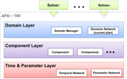
Fig. 1.The APSI-TRF architecture
The APSI-TRF architecture.
The APSI-TRF software consists of a layered architecture which is or-ganized according to the abstrac-tion level of the solving process. Broadly speaking, constraints are posted on the lower levels as a consequence of decisions taken on higher levels by analyzing variables in the underlying layers (for further details, the reader should refer to [7]).
The Time and Parameter Layeris the lowest layer of the APSI-TRF
archi-tecture and it is responsible of managing temporal and parameter information. It provides the functionalities for creating temporal and parameter elements, imposing constraints on them and querying the database to access information about events, temporal positions and parameter values. In particular, temporal information are managed in shape of Temporal Constraint Networks (TCNs). This layer is also endowed with propagation algorithms to maintain the consis-tency of the possible value assignments to time points. The current implementa-tion is based on theSimple Temporal Problem.The Component Layeris the point of expansion of the APSI-TRF architecture. A component is a module which en-capsulates the logic for computing a timeline resulting from decisions, evaluating the consistency of the computed timeline with respect to a set of given rules and computing a set of temporal and/or parameter constraints or new decisions to solve (if possible) any flaw for the consistency of the computed timeline. The
Domain Layeris responsible for managing decisions and relations among them.
This information are managed through a particular data structure called
Deci-sion Network. This layer is responsible for providing management functions and
generating synchronizations among components. TheDecision Networkprovides a unified vision of the current solution while the Domain Manager provides a unified means for expressing the constraints that the decisions must satisfy. A decision is a generic term to represent a choice with respect to the temporal evolution of the domain components and it constitutes the primitive operator to interact with them.
The APSI-TRF provides the timeline-based modeling primitives, to obtain a complete application that solves a particular problem, it is necessary to build a
problem solver on top of the framework. The Open Multi-Component Planner & Scheduler (Omps) [15], as implemented for theGoacproject [13] is an example of such solvers. It builds upon the APSI-TRF framework by selecting the domain components relevant to control and implements the solving engine able to find solution plans.
Limitations in APSI-TRF and Omps. After the deployment phase of the
Ompsplanner in theGoacproject, a further research effort has been provided
to enhance solver development within the APSI-TRF and, in particular, enabling the definition of general-purpose domain independent solvers. During theGoac
project, the main aim was to generate an effectiveP&Sapplication to address a particular problem and, more in general, the need of meeting operational re-quirements in challenging domains (like for instance the space context) often leads to the use of highly efficient software modules to address specific sub-parts of the problem with ad-hoc solving algorithms, while the need of reducing mod-eling mistakes leads to the need of involving users as much as possible in all the steps of software development.
This issue became more evident while applying that APSI-TRF application in solving problems different from the one for which it was developed (see Sec-tion 4.3). In fact, as applicaSec-tions are designed and implemented to focus on very complex problem contexts, the lack of generality is a reasonable payoff. Thus, the EPSL has been developed to enhance the current APSI-TRF solving structure exploiting the same representation layers. In fact, the EPSL has been built introducing amore general search structurerelying on the same APSI-TRF functionalities for managing and representing the domain timelines as well as on a set of operators (Resolvers) obtained by a decomposition of theOmpssolving process.
3
The Extensible Planning and Scheduling Library
The main goal of the Extensible Planning and Scheduling Library (EPSL) is to provide a planning environment in which it is possible to easily define and evaluate different solving configurations in order to find the best one for the particular problem to address.
3.1 Architectural Description
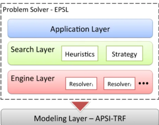
The EPSL can be seen as a solver which uses the APSI-TRF modeling func-tionalities described in Section 2.1 (see again Figure 1) to solve timeline-based problems. The new planning framework can be sketched as a layered architecture whose main elements are depicted in Figure 2.
Engine Layer. This lower layer manages a set of algorithms, calledResolvers
(inspired by the basic Omps solving process), that directly act on a timeline-based plan. Indeed, eachResolver is responsible to manipulate the plan in order to solve a particular kind of flaw (where aflaw identifies a condition which must
be removed to obtain a solution plan). So this layer provides a set of “ready-to-use” plan manipulation operators that can be combined together by the planner during the search. For the purpose of this paper, the operators that manipulate the timeline-based plan (implemented byResolvers) are the following:
Fig. 2.EPSL layered architecture
Decision Justification: It is the
pro-cess needed to safely introduce new decisions (goals) into the plan (a.k.a.
plan refinement). The introduction
of a decision into the plan induces on the associated components a parti-cular behavior on a certain time in-terval. So, the justification process guarantees the overall plan consis-tency by synchronizing the result-ing component’s behavior with other domain components.
State Variable Scheduling: It is the
process responsible to solve state variable value contention flaws. It allows to solve state variable inconsistencies due to partial overlapping of component de-cisions (a.k.a. values). We use the term scheduling because the timeline dede-cisions may be considered as activities containing “resource requirement” where the re-source (aState Variable) is abinary resource(a single value for each time instant is allowed). The contention flaws are solved by scheduling activities to achieve a total order among them (i.e., avoiding overlaps).
Timeline Extraction: It is the process that fixes floating time points on a
com-ponent (a state variable) so that a particular temporal evolution (a timeline) is decided for the component itself. Before the extraction step, plan decisions are not “fully ordered” so components may have several possible behaviors. The current extraction procedure uses anEarliest Start Time (EST) approach: each decision is allocated as soon as possible over its time bounds. It is worth re-minding that a valid behavior requires a completely allocated timeline in order to avoidunpredictable component behaviors.
State Variable Completion: It is the process responsible to solve state variable
gap flaws. It is an operator used, for example in thetimeline-extraction proce-dure. It completes a timeline when anytemporal gapis detected (agapis timeline time interval with no value assigned).
Search Layer. This is the layer for specifying planners in EPSL. It implements
the search process by coordinating and integrating together all elements that compose a planner instance. It is the “glue” among the set ofResolvers needed to refine the plan, the Heuristics used to analyze it and the Strategy used to manage the possible alternatives during the search.
Heuristics. This module is responsible for search node evaluation. It manages the specific knowledge about the problem in order to better support the solv-ing process, also providsolv-ing the facilities to easily define and integrate into the framework new heuristics. At present EPSL uses two classes of heuristics: (i)
Search-Heuristicidentifies the class of heuristics used for search space node
eval-uation in order to identify the most promising node to expand during solving process. (ii)Plan-Analyzer identifies the class of heuristics used forflaw selec-tion. So they have the responsibility to extract a set of flaws from the current partial plan, classify them and select the more relevant to solve in order to find a solution. Within EPSL, a basic search-heuristic implementation is defined as follows:
Definition 1. Given thatG(n) ={g0, g1, ..., gk}is the set of goalss of the
prob-lem status associated to the noden, the estimated cost solving the problem h(n)
computed by the heuristic function is:h(n) =P
g∈G(n) fi(g)wi,∀i∈OP where
OP is the set of primitiveoperators of the solving process, fi is the ith solving
step andwi is the associated cost.
Strategy. This module is responsible for managing the fringe of the search space.
A strategy defines a particular queuing policy of nodes not yet expanded and it may use an Heuristic function to better support the search process. The EPSL is endowed with a set of basic strategies, i.e.,A∗, Depth First Search (DFS) and Breadth First Search (BFS).
In addition, a probabilistic search strategy is provided. It consists of agreedy
search in which an evaluating function f(n) =P(n) is exploited representing a probabilistic distribution which expresses the probability of a node nto be the solution node, sof(n) =P(n)∈(0,1].
Definition 2. The probabilistic function P(n) is defined as:P(n) = eh(n)1 with
limh(n)→+∞eh(n)1 = 0 limh(n)→0+ 1
eh(n) = 1with h(n)∈[0,+∞).
The strategy sorts boundary nodes according to their probability values in order to extract first the nodes with the highest probability to be the solution.
Finally, the EPSL framework provides the capability of introducing either new search strategies or definingcomposite strategytaking advantage of a (sort of) composition operator to integrate different (already defined) search strate-gies.
Application Layer. This module represents theuser interfacewhich provides
functionalities for easily define and run new planning instances. A user can define a planner configuration by simply declare the elements composing the planner, then the framework is responsible to create the planner instance that the user can run to solve problem instances.
3.2 Main advantages in using EPSL
The EPSL design has been started in order to address the limitations discussed in Section 2.1. In fact, the APSI-TRF framework provides the possibility to effec-tively design applications relying on tailored solving structures but, in general,
they can not be easily (and quickly) deployed in different contexts. The main reason is that APSI-TRF currently allows the design and development of ap-plications relying on solvers strictly coupled with search strategy and heuristic information.
Then, as discussed above, EPSL provides an enhanced framework for devel-oping applications in which designers may focus on a single aspect of the solving process. In particular, EPSL allows to focus on (i) resolvers design (i.e., adding new reasoning capabilities), (ii) search strategies (i.e., possibly implementing additional algorithms) and (iii) heuristic functions definition (i.e., identifying suitable control strategies for the specific problem). All the above features con-cur in creating a portfolio of operators, algorithms and heuristics that actually enable the possibility to combine them in many possible ways (not only the ones for which they have been designed), then, providing application designers with a really flexible framework for P&S application development.
Finally, even though the EPSL is in an initial development stage, results collected after an experimental evaluation show that EPSL performances are comparable with Omps in the domain for which such APSI-TRF application has been developed (i.e., the GOAC domain). On the other hand, a particular EPSL planner (whose configuration has been identified after a fast assessment on the considered domain) shows better performances of Omps on a different planning domain elicited from a different space domain (see section 4.3).
4
Current Empirical Results
In this section, we present an experimental evaluation comparing EPSL and
Omps performances while solving different problem instances in two different
planning domains derived from real world scenarios: a robot control domain ex-tracted from the Goac project [13] and a space facility management domain extracted from the Ulisse project [17]. Before discussing empirical results, a brief description of the problem domains and their timeline-based representa-tions is provided. Then, experimental results are reported and discussed. All the experiments have been ran on a MacBook endowed with an Intel Core 2 Duo (2.26GHz) processor and 2GB RAM.
4.1 GOAC: A Robotic Domain
The Goal Oriented Autonomous Controller [13] is an ESA effort to create a common platform for robotic software development. In particular, the delivered GOAC architecture has integrated: (a) a timeline-based deliberative layer which integrates a planner based on the APSI Platform [7] and an executive a la T-REX [18]; (b) a functional layer which integrates GenoM and BIP [19].
The GOAC Domain. The robotic domain considers a planetary rover equipped
with a Pan-Tilt Unit (PTU), two stereo cameras (mounted on top of the PTU) and a communication facility. The rover is able to autonomously navigate the en-vironment, move the PTU, take pictures and communicate images to a Remote Orbiter. A safe PTU position is assumed to be (pan,tilt) = (0,0). Finally, during
the mission, the Orbiter may be not visible for some periods. Thus, the robotic platform can communicate only when the Orbiter is visible. The mission goal is a list of required pictures to be taken in different locations with an associated PTU configuration. A possible mission action sequence is the following: navigate to one of the requested locations, move the PTU pointing at the requested di-rection, take a picture, then, communicate the image to the orbiter during the next available visibility window, put back the PTU in the safe position and, fi-nally, move to the following requested location. Once all the locations have been visited and all the pictures have been communicated, the mission is considered successfully completed.
The rover must operate following some operative rules to maintain safe and effective configurations. Namely, the following conditions must hold during the overall mission: (C1) While the robot is moving the PTU must be in the safe position (pan and tilt at 0);(C2) The robotic platform can take a picture only if the robot is still in one of the requested locations while the PTU is pointing at the related direction; (C3)Once a picture has been taken, the rover has to communicate the picture to the base station;(C4) While communicating, the rover has to be still; (C5)While communicating, the orbiter has to be visible.
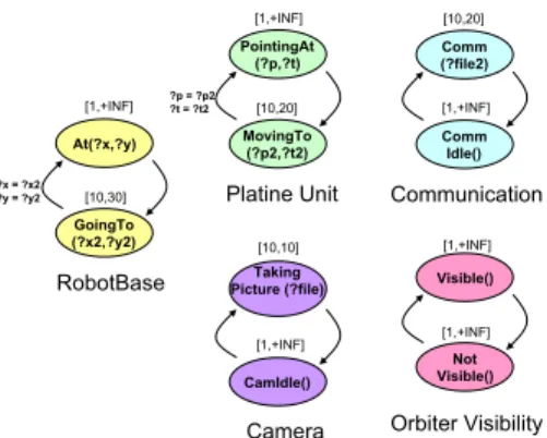
Taking Picture (?file) CamIdle() Camera Comm (?file2) Comm Idle() Communication PointingAt (?p,?t) MovingTo (?p2,?t2) ?p = ?p2 ?t = ?t2 Platine Unit At(?x,?y) GoingTo (?x2,?y2) ?x = ?x2 ?y = ?y2 RobotBase [1,+INF] [10,20] [1,+INF] [1,+INF] [1,+INF] [10,10] [10,20] [10,30] Visible() Not Visible() Orbiter Visibility [1,+INF] [1,+INF]
Fig. 3. State variables describing the robotic platform and the orbiter visibility (durations are stated in seconds)
Timeline specification for the
robotic domain. To obtain a
timeline-based specification of our robotic domain, we consider two types of state variables:Planned State
Vari-ablesto represent timelines whose
val-ues are decided by the planning agent,
andExternal State Variablesto
repre-sent timelines whose values over time can only be observed. Planned state variables are those representing time varying features like the temporal oc-currence of navigation, PTU, cam-era and communication opcam-erations. We use four of such state variables,
namely theRobotBase, PTU, CameraandCommunication.
In Fig. 3, we detail the values that can be assumed by these state variables, their durations and the legal value transitions in accordance with the mission requirements and the robot physics2 Additionally, one external state variable
represents contingent events, i.e., the communication opportunities. TheOrbiter
Visibility state variable maintains the visibility of the orbiter. The allowed
val-ues for this state variable is Visible or Not-Visible and are set as an external input. The robot can be in a position (At(x,y)) or moving towards a destination
(GoingTo(x,y)). The PTU can assume a PointingAt(pan,tilt) value if pointing
a certain direction, while, when moving, it assumes a MovingTo(pan,tilt). The camera can take a picture of a given object in a position hx, yiwith the PTU
2
Note that variables (e.g., ?x) represents parameters with values in a finite set of symbols, used to compactly represent the allowed values for a given state variable.
in hpan, tiltiand store it as a file in the on-board memory (
TakingPicture(file-id,x,y,pan,tilt)) or be idle (CamIdle()). Similarly, the communication facility
can be operative and dumping a given file (Communicating(file-id)) or be idle
(ComIdle()). Domain operational constraints are described by means of
synchro-nizations. A synchronization models the existing temporal and causal constraints
among the values taken by different timelines (i.e., patterns of legal occurrences of the operational states across the timelines).
0 Camera RobotBase Communication System GoingTo(1,4) At(0,0) At(1,4) MovingTo(30,-45) PointingAt(0,0) PointingAt(30,-45) CamIdle TakingPicture(obj,1,4,30,-45) CamIdle Off Communicating(file) Pan-Tilt DURING DURING BEFORE DURING DURING NotVisible Visible Visble
Orbiter Visibility DURING
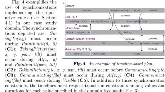
Fig. 4.An example of timeline-based plan.
Fig. 4 exemplifies the use of synchronizations implementing the oper-ative rules (see Section 4.1) in our case study domain. The synchroniza-tions depicted are:
Go-ingTo(x,y) must occur
during PointingAt(0, 0)
(C1); TakingPicture(pic,
x, y, pan, tilt) must
occur during At(x, y)
and PointingAt(pan, tilt)
(C2);TakingPicture(pic, x, y, pan, tilt)must occur beforeCommunicating(pic)
(C3); Communicating(file) must occur during At(x,y) (C4);
Communicat-ing(file) must occur during Visible (C5). In addition to those synchronization
constraints, the timelines must respect transition constraints among values and durations for each value specified in the domain (see again Fig. 3).
4.2 Testing Results on the GOAC Domain
This section investigates the EPSL planners performance by using our robotic case study as a benchmark. For this purpose, we introduce different planning problem scenarios obtained by varying the problem complexity along the follow-ing dimensions: plan lengthby playing on both the number of pictures (from 1 to 5) to be taken and the plan horizon; plan choices by changing the number of communication opportunities (from 1 to 4 visibility windows). Notice that an increasing number of communication opportunities raises the complexity of the planning problem with a combinatorial effect. More in general, among all the generated problem instances, the ones with higher number of required pictures and higher number of visibility windows result as the hardest ones. In these scenarios, we analyzed the performance of the planners.
Exploiting the flexibility provided by EPSL, we have easily configured five different planners in order to test the framework capabilities and also to compare their performances withOmps. Therefore, exploiting the strategies and heuris-tic functions described in Sec. 3.1, we have defined the following planners:BFS
Planner, A∗ Planner, Probabilistic Planner, and DFS Planner. In addition, a
more general planner, called Chronological Backtracking Planner, has been de-fined extending the DFS Planner using the Probabilistic Strategy described in Sec. 3.1.
This strategy splits the solving process in two phases. During the first phase, the planner uses the Probabilistic Strategy to apply the justification decisions,
then, the planner switch to theDFS Strategy in order to complete the plan and find a solution as soon as possible. Basically, this strategy provides a trade off between controlling the decisions to apply and completing the plan as quick as possible.
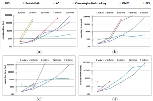
Moreover it is important to point out that EPSL features give the possi-bility to set several configuration parameters in order to affect planner choices during solution search. Therefore, Fig. 5 shows the results obtained by the best parameter configuration for each tested planner.
100 1000 10000 100000 1000000 1 picture
2 pictures 3 pictures 4 pictures 5 pictures
execu 1o n 1me ( ms ) 100 1000 10000 100000 1000000
1 picture 2 pictures 3 pictures 4 pictures 5 pictures
execu 1o n 1me ( ms ) (a) (b) 100 1000 10000 100000 1000000
1 picture 2 pictures 3 pictures 4 pictures 5 pictures
execu 1o n 1me ( ms ) 100 1000 10000 100000 1000000 1 picture
2 pictures 3 pictures 4 pictures 5 pictures
execu 1o n 1me ( ms ) (c) (d)
Fig. 5.EPSL testing results and comparison with OmpsonGoacproblem with: (a) one, (b) two, (c) three and (d) four communication windows.
The resulting performances demonstrate how different planner configurations may lead to pretty different results. The BFS Planner is the worst among the defined EPSL planners as it is able to solve few problem instances. Indeed, using such strategy leads to expand a lot of nodes before a solution is found, possibly because the problem domain structure determines very deep solution nodes. So, in this case, the planner spends a lot of time in expanding nodes and in maintainingTemporal Network consistency without approaching the solution node. This is also confirmed by the fact thatA∗ Planner has performances very close to those of theBFS Planner. This also allows us to argue that the exploited
heuristic function is not informed enough.
On the other hand, theDFS PlannerandOmpsresults as the best planners (see again Fig. 5). In fact, both use a strategy that does not make an evaluation of boundary nodes during the search. They always make the same choices (decision expansion) during the search. Given the characteristics of the GOAC problem, this results as the best approach as they are able to manage in a more effective way the underlyingTemporal Network, thus, reducing thepropagation cost due to the maintenance of temporal constraint consistency. However, such planners
do not provide any control on the solving process and, as we will see in the next section, this is not a good behavior for different kind of problems.
As a final remark, EPSL does not always offer performances better than
Omps. In particular, onlyDFS Planner is comparable toOmps(even better in
some cases). However, it is important to notice that the main goal of the system is to realize a flexible and extensible software library by which it is possible to easily define new planning instances or to adapt an already defined planner to a particular problem. Indeed, EPSL unlikeOmpsgives the possibility to focus the efforts on specific aspects of solving process so by means of its functionalities it is possible, for instance, to improve solution search by providing a more informed heuristic as well as to improve theTemporal Network management by providing more efficient algorithms.
4.3 FSL: A Space Facility Management Domain
The ”USOCs Knowledge Integration and dissemination for Space Science Ex-perimentation” (ULISSE) is a project (funded by EU and indicated by REA as example of successful FP7 project in the Space field) whose objective is data val-orization around the ISS experiments. Each USOC (User Support and Operation Centre) is responsible for a particular on-board facility that is to be operated to perform scientific experiments and to generate the related scientific data. Here, we report a simplified planning domain derived from the one described in [17] aiming at addressing a short-term planning problem in managing a particular ISS facility.
The Fluid Science Laboratory. The FSL is a ISS multi-user facility designed
for the execution of experiments on fluid physics under microgravity conditions. The FSL is equipped with a number of optical instruments that allow to sepa-rately implement a wide variety of diagnostic techniques that can be combined together and each combination is calledoptical mode. Generally, an experiment execution consists of several runs, a run is a part of the experiment that uses a defined configuration and setting of the facility (as for example a specific optical mode). The data recorded by the experiments are sent in a real-time manner to the ground. Data is routed to the Columbus for communicating to the ground through a High Rate downlink channel mainly intended for high rate science data. The FSL is always in one defined status, among the following: Off, Stand-by, Configuration & Checkout and Nominal. A set of operations on FSL has been identified that require an initial status of FSL and may eventually lead to a transition to a new status of the facility. Each activity is characterized by several parameters, e.g., the team that operates the FSL, the duration of the activity, etc. A complete specification of the FSL activities is given in [17].
Each plan executed on the FSL has to comply with a set of operative con-straints. These are related to general operational requirements: prior to per-forming scientific experiments and/or diagnostic tests correctly, the FSL must follow a precise sequence of steps in order to be fully operative: initially, it must be mechanically configured according to the experiment/test to be performed; subsequently, the operative rack has to be activated; finally, the set of diagnos-tics must be executed before the experiment can commence. At the end of each
operative cycle, the previous operations must be planned to be executed in the reverse order. At the beginning of each operative period, an optical mode test has to be performed to check whether the mechanical configuration has been cor-rectly completed (avoiding to perform experiments with optical targets wrongly set); the High Rate Data Link (HRDL) has to be allocated during each run that requires real time data transmission; a run cannot be interrupted and has to be executed continuously. Finally, other operative constraints are required for safety issues: during non operative periods, the status of both the FSL and the Rack must be off, FSL mechanical configuration and de-configuration activities have to be performed with both FSL Rack and FSL switched off.
Generally, the execution of an experiment consists of several runs; a run is a segment of the experiment that uses a defined configuration and setting of the facility (as for example a specific optical mode). The objective function for the problem is that all the planned experiments must be performed and the recorded activities should be safely downloaded on ground stations.
A timeline specification for the FSL domain. To obtain a timeline-based
specification of the FSL domain a set ofmulti-valued state variableshas been con-sidered. Configured Deconfigured Mechanical configuration On Off Rack Off StandBy CC FSL FSL_Activities OPT_TGT_INST(x) OPT_TGT_RMV FSL_CC RACK_ACT FSL_STBY RACK_DEACT RT_OPT_CO(z) DATA_DNLK IDLE [10,10] [25,25] [40,40] [10,10] [15,15] [20,20] [300,300] [50,50]
Available Not Available
HDRL
Fig. 6.Value transitions for state variables describ-ing the FSL (temporal durations in minutes). Multi-valued state
vari-ables are those representing time varying feature for the temporal occurrence of me-chanical configurations, rack activations as well as both FSL status and activities. In this regard, we consider four different state variables, i.e., Mechanical
Configura-tion,Rack,FSLandFSL
Acti-vities. The Figure 6 depicts
a detailed view of the val-ues that can be assumed by these state variables, their
du-rations and the allowed value transitions in accordance with the operative con-straints.
In general, before any operative period, the FSL requires aMechanical
Con-figuration. In particular, during not operative period no optical target is mounted
on the FSL (Deconfigured) while, before starting an optical checkout, a suitable optical target is to be mounted to result mechanically configured (Configured). The Rackcan assume a Active status when switched on while, when switched off, it assumes aNot Activevalue. The FSL can assume different status as well as perform different activities. TheFSLmay be in one of the following status:Off
while not operating, StandBy after initialization and in operative mode when ready for Control and Checkout (i.e., CC). The FSL Activities represents the full set of activities that can be performed on-board. Namely, the FSL activi-ties are the following: installation or removal of an optical target (respectively,
OPT TGT INST(x) and OPT TGT RMV with x representing one of the 86 available optical modes); activation and deactivation of the rack (RACK ACT
and RACK DEACT); initialization and activation of the optical component
(FSL STBY andFSL CC); finally, while running an optical checkout the FSL
may assume the RT OPT CO(x); finally, executing a downlink activity results in assuming the DATA DNLK value. In Figure 6, we detail the values that can be assumed by these state variables, their durations and the allowed value transitions in accordance with the operative requirements.
In the FSL domain, the following compatibilities are considered (not shown in Figure 6 not to overload the representation): (1) OPT TGT INST values must occur DURING a Deconfigured value on the Mechanical Configuration variable; (2) OPT TGT RMV as well as Active and RACK ACT must occur DURING a Configured value on the Mechanical Configuration state variable;
(3)RACK DEACT,RACK STBY andRACK CC must occur DURING a
Ac-tivevalue on the Rack state variable; (4) RT OPT COandDATA DNLKmust occur during a CC value on the FSL state variable. The first two compati-bilities globally express the circumstance that all FSL activities must be per-formed within a Rack activation/deactivation cycle, and that such cycle must be performed once an optical target has been configured. The third compatibility enforces that the FSL is supposed to be initialized before being fully operative. Finally, constraint (4) enforces that the main FSL activities should be performed while in CC.
4.4 Testing Results on the FSL Domain
This section further investigates the performances of the EPSL in the FSL case study. Again, we consider different planning problem scenarios obtained by vary-ing the problem complexity by varyvary-ing: (1) plan length, i.e., both the number of optical check out (from 1 to 30) to be taken and the plan horizon; (2) Plan
Flexibility, i.e., for each FSL activity, we set a minimal duration, but allow
tem-poral flexibility on the activity termination, namely, the end of each activity has a tolerance ranging from 0 to 30 seconds. This temporal interval represents the degree of temporal flexibility/uncertainty that we introduce in the system. It is worth to underscore that, among all the generated problem instances, the ones with higher number of required pictures and higher temporal flexibility corre-spond to the hardest ones. In these scenarios, we analyzed the performance of the planners but, here, rather than testing all the possible EPSL planners as in the previous case study, we exploited the Chronological Backtracking Planner
configuration already defined for the GOAC problem (see Sec. 4.2) taking ad-vantage of the EPSL flexibility to quickly configure the more suitable planner to test the framework as well as to compare its performance withOmps.
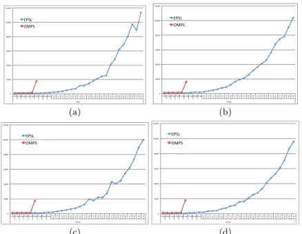
In this case, the EPSL PlannerdominatesOmps(see Fig. 7) providing best performances in every configuration. In this domain, there are different kind of choices (decisions for unification) that must be applied in order to efficiently find a solution and, in this regard,Ompssolving settings can not be adjusted in order to change its solving behavior. Therefore,Ompsapplies the same solving approach (i.e., a fully DFS strategy) as for the GOAC domain, while EPSL exploit the possibility to control the application of justification decisions during
0 20000 40000 60000 80000 100000 120000
1 exp 2 exp 3 exp 4 exp 5 exp 6 exp 7 exp 8 exp 9 exp 10 exp 11 exp 12 exp 13 exp 14 exp 15 exp 16 exp 17 exp 18 exp 19 exp 20 exp 21 exp 22 exp 23 exp 24 exp 25 exp 26 exp 27 exp 28 exp 29 exp 30 exp 0 flex EPSL OMPS 0 20000 40000 60000 80000 100000 120000
1 exp 2 exp 3 exp 4 exp 5 exp 6 exp 7 exp 8 exp 9 exp 10
exp exp 11 exp 12 exp 13 exp 14 15 exp exp 16 17 exp exp 18 19 exp exp 20 21 exp exp 22 exp 23 exp 24 exp 25 26 exp exp 27 28 exp exp 29 30 exp 10 flex EPSL OMPS (a) (b) 0 20000 40000 60000 80000 100000 120000
1 exp 2 exp 3 exp 4 exp 5 exp 6 exp 7 exp 8 exp 9 exp 10
exp exp 11 exp 12 exp 13 exp 14 exp 15 16 exp exp 17 18 exp exp 19 exp 20 exp 21 22 exp exp 23 exp 24 exp 25 exp 26 27 exp exp 28 29 exp exp 30 20 flex EPSL OMPS 0 20000 40000 60000 80000 100000 120000
1 exp 2 exp 3 exp 4 exp 5 exp 6 exp 7 exp 8 exp 9 exp 10 exp 11 exp 12 exp 13 exp 14 exp 15 exp 16 exp 17 exp 18 exp 19 exp 20 exp 21 exp 22 exp 23 exp 24 exp 25 exp 26 exp 27 exp 28 exp 29 exp 30 exp 30 flex EPSL OMPS (c) (d)
Fig. 7.EPSL comparison withOmps(time in msecs.) on ULISSE problem with: (a) 0 seconds flex.; (b) 10 seconds flex.; (c) 20 seconds flex.; (d) 30 seconds flex..
the search, thus, providing a search strategy that allows the planner to efficiently address the FSL problem. As discussed in Sec. 2.1, this is an expected behavior. In fact,Ompshas been designed and developed to face different planning domain and problem instances. Thus, given its structure, it would require additional design efforts in order to address also the FSL management.
5
Conclusion
This paper has introduced EPSL a tool that represents an advancement in devel-oping an extensible and general-purpose planning environment using the same APSI-TRF interfaces. The system aims at providing the possibility to focus on specific aspects (e.g. heuristic or strategy definition) taking advantage of the flexibility of the implemented timeline-based solving process. The evalua-tion presented in this paper shows how it can be used for synthesizing domain independent planners. Such planners have been evaluated with respect to two real-world application domains against the preheating Omps planner as devel-oped for the Goacproject. We have shown how the EPSL-based planners are comparable withOmpson theGoacdomain and outperform it on FSL. Some-how this represents the basic seed result for justifying our research. We will now continue our work comparing with other possible approaches (e.g., EUROPA) but also pursuing further enhancements of EPSL to integrate state of the art technology for domain-independent search control.
Acknowledgments. Authors are supported by CNR under the GECKO Project
References
1. Muscettola, N.: HSTS: Integrating Planning and Scheduling. In Zweben, M. and Fox, M.S., ed.: Intelligent Scheduling. Morgan Kauffmann (1994)
2. Jonsson, A., Morris, P., Muscettola, N., Rajan, K., Smith, B.: Planning in Inter-planetary Space: Theory and Practice. In: AIPS-00. Proc. of the Fifth Int. Conf. on Artificial Intelligence Planning and Scheduling. (2000) 177–186
3. Cesta, A., Cortellessa, G., Fratini, S., Oddi, A., Policella, N.: An Innovative Prod-uct for Space Mission Planning: An A Posteriori Evaluation. In: ICAPS-07. (2007) 4. Frank, J., Jonsson, A.: Constraint Based Attribute and Interval Planning. Journal
of Constraints8(4)(2003) 339–364
5. Bernardini, S.: Constraint Based Temporal Planning: Issues in Domain Modeling and Search Control. PhD thesis, Universita degli studi di Trento (2008)
6. Chien, S., Rabideau, G., Knight, R., Sherwood, R., Engelhardt, B., Mutz, D., Estlin, T., Smith, B., Fisher, F., Barrett, T., Stebbins, G., Tran, D.: ASPEN -Automated Planning and Scheduling for Space Mission Operations. In: Proc. of SpaceOps 2000. (2000)
7. Cesta, A., Cortellessa, G., Fratini, S., Oddi, A.: Developing an End-to-End Plan-ning Application from a Timeline Representation Framework. In: IAAI. Proc. of the 21st Conference on Innovative Applications of Artificial Intelligence. (2009) 8. Smith, D., Frank, J., Jonsson, A.: Bridging the Gap Between Planning and
Sched-uling. Knowledge Engineering Review15(1) (2000) 47–83
9. Laborie, P., Ghallab, M.: IxTeT: an integrated approach for plan generation and scheduling. In: ETFA: Emerging Technologies and Factory Automation. (1995) 10. Chien, S.A., Johnston, M., Frank, J., Giuliano, M., Kavelaars, A., Lenzen, C.,
Policella, N.: A Generalized Timeline Representation, Services, and Interface for Automating Space Mission Operations. In: SpaceOps. (2012)
11. J´onsson, A.K., Morris, P.H., Muscettola, N., Rajan, K., Smith, B.: Planning in interplanetary space: Theory and practice. In: ICAPS. (2000) 177–186
12. Cesta, A., Cortellessa, G., Fratini, S., Oddi, A.: MrSPOCK: Steps in Developing an End-to-End Space Application. Computational Intelligence27(1) (2011) 13. Ceballos, A., Bensalem, S., Cesta, A., de Silva, L., Fratini, S., Ingrand, F., Ocon,
J., Orlandini, A., Py, F., Rajan, K., Rasconi, R., van Winnendael, M.: A Goal-Oriented Autonomous Controller for Space Exploration. In: ASTRA-11. 11th Sym-posium on Advanced Space Technologies in Robotics and Automation. (2011) 14. Fratini, S., Cesta, A., De Benidictis, R., Orlandini, A., Rasconi, R.: APSI-based
deliberation in Goal Oriented Autonomous Controllers. In: ASTRA-11. 11th Sym-posium on Advanced Space Technologies in Robotics and Automation. (2011) 15. Fratini, S., Pecora, F., Cesta, A.: Unifying Planning and Scheduling as Timelines
in a Component-Based Perspective. Archives of Control Sciences18(2) (2008) 16. Cesta, A., Oddi, A.: DDL.1: A Formal Description of a Constraint Representation
Language for Physical Domains,. In Ghallab, M., Milani, A., eds.: New Directions in AI Planning. IOS Press: Amsterdam (1996)
17. Carotenuto, L., Ceriello, A., Cesta, A., Benedictis, R.D., Orlandini, A., Rasconi, R.: Planning and Scheduling Services to Support Facility Management in the ISS. In: 63rd International Astronautics Congress, IAC-12-B5.2.10., Naples, IT. (2012) 18. Py, F., Rajan, K., McGann, C.: A Systematic Agent Framework for Situated Autonomous Systems. In: AAMAS-10. Proc. of the 9thInt. Conf. on Autonomous Agents and Multiagent Systems. (2010)
19. Bensalem, S., de Silva, L., Gallien, M., Ingrand, F., Yan, R.: “Rock Solid” Soft-ware: A Verifiable and Correct-by-Construction Controller for Rover and Space-craft Functional Levels. In: i-SAIRAS-10. Proc. of the 10thInt. Symp. on Artificial Intelligence, Robotics and Automation in Space. (2010)