An efficient reliability analysis on complex non-repairable systems with common-cause failures

Safety and Reliability – Safe Societies in a Changing World – Haugen et al. (Eds) © 2018 Taylor & Francis Group, London, ISBN 978-0-8153-8682-7

An efficient reliability analysis on complex non-repairable systems

with common-cause failures

G. Feng

Department of Engineering Mathematics, University of Bristol, Bristol, UK

H. George-Williams

Institute for Risk and Uncertainty, University of Liverpool, Liverpool, UK

Institute of Nuclear Engineering and Science, National Tsing Hua University, Hsinchu, Taiwan

E. Patelli

Institute for Risk and Uncertainty, University of Liverpool, Liverpool, UK

F.P.A. Coolen

Department of Mathematical Sciences, Durham University, Durham, UK

M. Beer

Institute for Risk and Reliability, Leibniz University Hannover, Hannover, Germany Institute for Risk and Uncertainty, University of Liverpool, Liverpool, UK

School of Civil Engineering and Shanghai Institute of Disaster Prevention and Relief, Tongji University, China

ABSTRACT: Common-Cause Failures (CCF) impose severe consequences on a complex system’s reli-ability and overall performance. A more realistic assessment, therefore, of the survivreli-ability of the system requires an adequate consideration of these failures. The survival signature approach opens up a new and efficient way to compute system reliability, given its ability to segregate the structural and probabilistic attributes of the system. Traditional survival signature-based approaches assume the failure of one com-ponent to have no effect on the survival of the others. This assumption, however, is flawed for most realis-tic systems, given the existence of various forms of couplings between components. This paper, therefore, presents a novel and general survival signature-based simulation approach for non-repairable complex systems. We have used Monte Carlo Simulation to enhance the easy propagation of CCF across the com-plex system, instead of an analytical approach, which currently is impossible. In real application world, however, due to lack of knowledge or data about the behaviour of a certain component, its parameters can only be reported with a certain level of confidence, normally expressed as an interval. In order to deal with the imprecision, the double loop Monte Carlo simulation methodology which bases on the survival signature is used to analyse the complex system with CCF. The numerical examples are presented in the end to show the applicability of the approach.

the reliability and availability of multi-component systems. They are, therefore, extremely impor-tant in reliability assessment and must be given adequate treatment, to minimise overestimation (Modarres 2006).

The CCF event can either impact the overall sys-tem operation or only affect specific components within the system (Wierman et al. 2007). Aldemir (1987) haa given an overview of parametric Com-mon-Cause Failure models. To be specific, for com-ponent level, the CCF event is a comcom-ponent level failure. Rasmuson and Kelly reviewed the basic concepts of modelling CCFs in reliability and risk 1 INTRODUCTION

Common-Cause Failures (CCFs) are failure events that affect multiple components simultaneously. The origin of common cause events can be out-side the system components they affect, or they can originate from the components themselves, causing the other components to fail. The proper consideration and modelling of CCFs is essential in complex systems reliability analysis, as they may have a significantly adverse effect on the system’s overall functionality. They have been shown by many studies (Dhillon & Anude 1994) to decrease

studies (Rasmuson & Kelly 2008). One of the most commonly used single parameter models defined by Fleming (1975) is the β-factor model, which is the first parameter model applied to common cause failures in risk and reliability analysis. He then generalised the β-factor model to the multiple Greek letter model in 1986 (Fleming et al. 1986). The α-factor model which is proposed by Mosleh et al. (1988) develops CCFs from a set of failure ratios and the total component failure rate. Based on the α-factor model, Kelly & Atwood (2011) presented a method for developing Dirichlet prior distributions that have specified marginal means, but which are otherwise minimally informative. The binomial failure rate model (Atwood 1986) on the other hand, estimates the failure frequency of two or more components in a redundant system. This is computed as the product of the CCF shock arrival rate and the conditional failure probability of the components given the shock.

At for system level, the CCF event is a system functional level failure. A number of models have been developed recently. For instance, George-Wil-liams & Patelli (2017) proposed an efficient load-flow simulation approach to assess the availability of reconfigurable multi-state systems with inter-dependencies. A robust Bayesian approach to the α-factor model for common cause failures has also been proposed by Troffaes et al. (2014). Coolen & Coolen-Maturi (2015b) presented a non-para-metric predictive inference for system reliability following a common cause failure. However, there are mainly two problems within the above research works: (1) either recognise the components within the system as exchangeable single type; or (2) evaluate the system configuration for every reli-ability estimation trial, which is time consuming. Therefore, an extension of above works is needed. To be specific, it is necessary to perform reliability analysis on systems susceptible to CCFs, because these realistic complex systems always consist of components which belong to different types. Sur-vival signature provides a good way to solve this problem.

Survival signature was first proposed by Coolen & Coolen-Maturi (2012) in 2012. It is a powerful methodology which can not only hold the merits of the former system signature (Samaniego 2007), but can be used in complex system with components belong to multiple types. In essence, it does not have the assumption that components of different types are exchangeable, which overcomes the long-standing limitation of the system signature. This is useful when a system consists of components that belong to different types, which means their failure times follow different probability distribu-tions characters (Coolen & Coolen-Maturi 2015a). Therefore, survival signature is a promising method

for application to complex systems. Based on the former work, Aslett et al. (2015) analysed system reliability within the Bayesian framework of sta-tistics. Feng et al. (2016) dealt with the imprecision within the system by analytical and numerical ways respectively, what is more, new component impor-tance measures were presented in this paper. An imprecise Bayesian non-parametric approach by using sets of priors to system reliability with multi-ple types of components was developed by Walter et al. (2017). Patelli et al. (2017) proposed efficient simulation approaches which based on survival signature for reliability analysis on large system. Reed (2017) put forward an efficient algorithm for exact computation of survival signature using binary decision diagrams.

This paper is organised as follows. Section 2 gives a brief conceptions about the survival signature and α-factor parameter. The survival signature-based simulation reliability approach is proposed in Section  3, in addition, this Section introduces imprecision within the components failure times. The applicability and performance of the proposed approaches is presented in Section 4. Finally Sec-tion 5 closes the paper with conclusions.

2 SURVIVAL SIGNATURE AND

α

-FACTOR PARAMETER

2.1 Survival signature

Suppose there is a complex system with m

components which belong to K≥ 2 component types, with mk components of type k∈

{

1 2, ,...,K

}

and

mk m

k K

=

=

∑

1 . Assume that the random failure times

of components of the same type are exchangeable, while full independence is assumed for compo-nents belong to different types (iid), the survival signature which can be denoted by Φ

(

l l1 2, ,..., ,lK

)

with lk=0 1, ,...,mk for k=1 2, ,..., . It defines K

the probability that the system functions given that lk of its mk components of type k work, for

each k∈

{

1 2, ,...,K

}

. There are m_lk k    state vec-tors xk _{with x l} ik k i mk ₌ =

∑

1 (k = 1, 2, …, K), where xk x xk k x mkk

=

(

1, ,...,2

)

. Let Sl l1 2, ,...,lK denote the set of

all state vectors for the whole system, and it can be known that all the state vectors xk S

lkk ∈ are equally likely to occur. Therefore, the survival sig-nature can be expressed as:

Φ l l m l x K k K k k x Sl lK 1 1 1 1 ,..., ,...,

(

)

=            ×

( )

= − ∈

∏

∑

φ (1)

where φ φ=

( )

x _{:{ , }0 1}m→

{ }

_{0 1 is the system struc-,}

possible state vectors x. φ is 1 if the system func-tions for state vector x and 0 if not.

Let C tk

( )

∈

{

0 1, ,...,mk

}

denote the number of

k components working at time t. Assume that the components of type k have a known cumulative distribution function (CDF) Fk(t) and the

compo-nents failure times of different type are assumed independent, then: P C t l P C t l m l F t k k k K k K k k k K k k k m ( { }) ]

( )

= =

(

( )

=

)

=    

( )

= = =

∏

∏

1 1 1

∩

kk lk k k l F t −   −1

( )

] (2)

Hence, the survival function of the system with

K types of components becomes:

P T ts l l P C t l l m l m K k k k K K K ( > =) ...

(

,...,

)

 {

( )

= }    = = =

∑ ∑

1 1 0 0 1 1 Φ

_∩

_ (3) Equation 3 shows that the structure of the sys-tem is separated from the its components failure times, which is the typical advantage of the sur-vival signature. The sursur-vival signature is a sum-mary of structure functions and only needs to be calculated once for the same system. As a result, it is an efficient method to perform system reliability analysis on complex systems with multiple compo-nent types.

2.2 α-factor model

The α-factor model is particularly useful in the practical engineering world as the alpha factor parameters can be got through experts’ judgement of the system or past data on the system.

The parameter, αr, of the model, is the

frac-tion of the total component failure events caus-ing the simultaneous failure of an additional r – 1 components.

Let us assume there is a system with three exchangeable components, α1 means the failure of

one component cannot influence the status of the other components. α3 denotes the failure of one

component can lead to the other two components fail simultaneously, which means CCFs occur. For α2=p, it expresses that there is a probability p of

one additional component failing, following the failure of a component in this system. It can be drawn that

∑

_r=1αr=1

3

.

Similarly, for the complex system with multi-ple component types, the alpha parameters αrk

denotes that if one component of type k fails due to an common cause event, the probability that the other r – 1 components fail simultaneously. If there

are mk components in this group, it can conclude

that _r αrk

mk ₌

=

∑

₁ 1.

Based on the definition of α-factor parameter, the probability of a common cause basic event involving failure of k components in a system of m

components can be calculated by Equation 4.

Q k m k Q k k t t = − −     1 1 α α (4) where, k=1 2, ,..., and m αt _k αk m k =

∑

₌₁ .Qt is the

total probability of failure accounting both for common cause failures and independent failures. The alpha parameter estimator can be expressed as:

αk k i m i n n = =

∑

1 (5) where, nk is the number of events with k failed

components.

The α parameter estimator represents the prob-ability that exactly k of the m components fail, given that at least one failure has occurred. It can be seen from Equation  5 that the sum of all the αk will be 1. The advantage of the α-factor model

is its distinction between the total failure rate of a component Qt, for which we generally have a lot of

information, and common cause failures modelled by αk, for which we generally have very little

infor-mation (Troffaes et al. 2014).

3 EFFICIENT METHOD FOR ANALYSING SYSTEM RELIABILITY WITH COMMON CAUSE FAILURES

3.1 The proposed approach

In order to perform reliability assessment on any kind of systems without introducing simplifica-tions or unjustified assumpsimplifica-tions, this Section proposes a simulation method to analyse system reliability after common cause failures.

Suppose there is a complex system with m com-ponents which belong to Xc different component

groups, and there are mk components of type

k∈

{

1 2, ,...,K

}

and _k mk m

K

=

=

∑

₁ . The common cause group matrix can be expressed as MCCG, the

α factor parameters of each component group, αmkk, are stored in the matrix, recall αm

k k K k= =

∑

₁ 1.

The number of failing component of each type is depended on the number of component still func-tioning, therefore, it is necessary to use the α-factor model to provide probabilities for any combina-tions of number of components that would fail

when a common cause failure event occurs. Here has an assumption that if one component of type

k fails, it can only influence the components within the same component group Xc under the CCF

model. This is reasonable as the components of the same type tend to be influenced by the same com-mon cause failure event, this is also the reason why they are grouped in the same type. Then looking at how many of the components of each type still function, and assume exchangeability within them with regard to the CCF failure model.

The reliability of the system after common cause failures can be estimated adopting the fol-lowing simulation procedure:

Step 1. Initialise the counter V to store the out-put, define the mission time as tm and

number of samples as N;

Step 2. Define the component groups as Xc, and

the common cause group matrix MCCG,

the α factor parameters αmkk are stored

in the matrix;

Step 3. Sample the failure time of each compo-nent as ti≤ti+1, where i= 1, 2, …, m, and

set told= 0, at this time the survival

signa-ture (production level) is equal to 1; Step 4. Set the current time tcurrent=min(ti);

Step 5. At time ti, finding out which component

fails and which common cause group it belongs to. The components affected by a failure event due to CCF can be expresses as Vcomp;

Step 6. Upgrade the number of working compo-nents of each component group after the CCF, and then get the survival signature (production level) Φ_ti after the corres pon-ding failure time ti;

Step 7. Set the failure time of the components (the failure component and its common cause failure components) as infinite; Step 8. Repeat Steps 4 through 7 until tm>told;

Step 9. Store the production level of the system over the time by V j

( )

=V j

( )

+ Φti;

Step 10. Repeat Steps 3 through 9 for N times. Therefore, the survival function of the complex system after common cause failures is obtained by averaging the vector collecting the production level of the system over the number of samples:

P T t CCF( s> | )=V Nt/ .

The algorithm of the proposed simulation method can be seen follows:

3.2 Imprecision in consideration

In the engineering applications, if there exist impre-cision within the components failure time distri-butions, or empirical distribution of components failure times are used, no analytical methods can be

used without resorting to some degree of simplifica-tion or approximasimplifica-tion (Beer et al. 2013) (Aven 2017). Instead, the proposed simulation methods can be applied to any systems irrespectively to the probabil-ity distribution for the component failure time used. To be specific, the system reliability perform-ance after common cause failures can be simu-lated using survival signature-based Monte Carlo method. This double loop simulation method (Du & Chen 2004) not only has the advantage of sur-vival signature to handle complex system reliability problems, but can recur to Monte Carlo simulation to deal with the uncertainties within the system.

Double loop sampling involves two layers of sampling: the outer loop is called the parameter

loop since it concerns sampling different values for the set of distribution parameters for all of the uncertain quantities; while the inner loop goes by the name of probability loop because it involves sampling from precise probability distribution func-tions. As a matter of fact, double loop sampling implicates sampling from an analytical distribution whose parameters have been generated by sampling.

To solve the parameter epistemic imprecision within components, it is just need to add an opti-mization loop around the survival signature-based simulation method cited in Section 3.1 to estimate the bounds. In other words, it can be done by add-ing a simple Monte Carlo loop and sampladd-ing the values of components parameters from uniform distributions.

4 NUMERICAL EXAMPLE

Shown in Figure 1 is an arbitrary 13-component complex system, which components are arranged into five groups. The number within each box denotes which group the component belongs to while the number outside defines the index of the component in the system. The system is assumed to be non-repairable and components of the same group have the same failure time distribution, as defined in Table 2. In the table, an exponential dis-tribution is defined by its mean (in hours) while a Weibull distribution is defined by a set which first element is its scale parameter (in hours).

The system is first analysed without CCF using the proposed simulation model with the data presented in Table 2 and compared to its analytical solution.

It is then re-analysed considering common cause failures with all common cause groups are active. For this system, the common cause group failure matrix MCCG, with and without CCF, can

be expressed in Equations 6 and 7 respectively. The results obtained are shown in Figure 2.

MCCG=   0 95 0 05_{0 8 0 1 0 05 0 05}0 0 1 0 0 0 0 9 0 1 0 0 0 75 0 1 0 1 0 05 . . . . . . . . . . . .              (6)

Figure  1. Complex system with thirteen components which belong to four types. The number inside the com-ponent box represents the type, while the number outside the box expresses the component index.

Table 1. Component failure data with precise distribu-tion parameters.

Compo-nent

type Distribution type Distribution parameters CCF parameters

1 Weibull (1.8,2.2) {0.95, 0.05}

2 Exponential 1.2 {0.8, 0.1, 0.05, 0.05}

3 Weibull (2.3,1.6) {1}

4 Weibull (3.2,2.6) {0.9, 0.1}

5 Exponential 2.1 {0.75, 0.1, 0.1, 0.05}

Table 2. Component failure data with imprecise distri-bution parameters.

Component

type Distribution type Distribution parameters CCF parameters

1 Weibull ([1.68,1.86], [2.08,2.32]) {0.95, 0.05} 2 Exponential [1.07,1.33] {0.8, 0.1, 0.05, 0.05} 3 Weibull ([2.12,2.51], [1.38,1.72]) {1} 4 Weibull ([2.99,3.41], [2.51,2.79]) {0.9, 0.1} 5 Exponential [2.01,2.28] {0.75, 0.1, 0.1, 0.05}

Figure 2. Survival function of the system in Figure 1

with CCF and without CCF through simulation method, along with the system reliability without CCF got by ana-lytical solution.

MCCG=                 1 0 0 0 1 0 0 0 1 0 0 0 1 0 0 0 1 0 0 0 (7)

The accuracy and generality of the proposed simulation approach are validated by the plots in Figure 2, given the agreement between the simula-tion and analytical results. As shown, the reliability of the system reduces drastically when the effects of CCF are factored into the analysis. It exempli-fies the need to consider this realistic aspect of a system’s operation in its reliability evaluation.

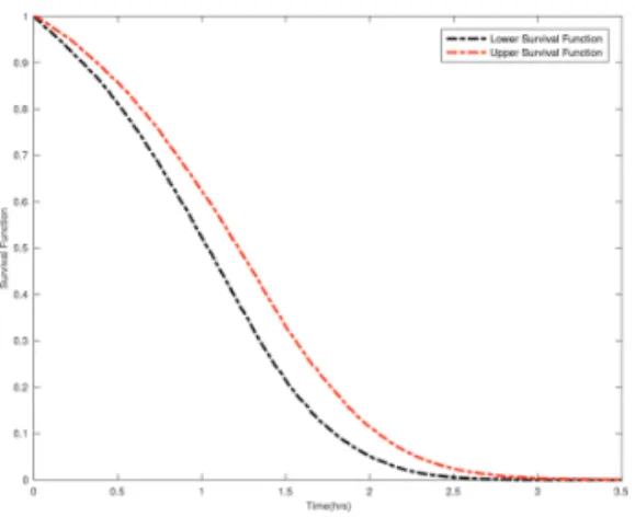
To deduce the effects of imprecision in the fail-ure distribution parameters of components on the system survival function, the system is analysed using the data presented in Table  2. Instead of a single curve, the survival function, in this case, could be any of an infinite number of curves lying within the bounds shown in Figure 3.

5 CONCLUSIONS

Common-Cause Failures (CCF) have an adverse effect on the reliability and performance of multi-component systems. They are normally a conse-quence of functional couplings between a group of components due to a variety of possible reasons. Thus, there is an inevitability about the suscepti-bility of realistic multi-component engineering systems to these failures. The need, therefore, to incorporate CCF considerations into system anal-ysis is overwhelming, as the alternative may lead to overestimating the reliability of the system.

This paper puts forwards an efficient simulation method which bases on the survival signature to

perform reliability analysis on complex systems with common cause failures. In fact, this approach extends the applicability of the survival signature approach to systems susceptible to common cause failures. More importantly, it holds the merits of both survival signature methodology and Monte Carlo simulation. Therefore, this approach is gen-eral and allows to know the survival function of the system after common cause failures at each time. What is more, the probabilistic uncertainty and imprecision in components parameters are taken into consideration by resorting this general simu-lation method. The effectiveness and feasibility of the proposed approach hasbeen demonstrated by the numerical example.

REFERENCES

Aldemir, T. (1987). Computer-assisted markov failure

modeling of process control systems. IEEE

Transac-tions on reliability 36(1), 133–144.

Aslett, L.J., F.P. Coolen, & S.P. Wilson (2015). Baye-sian inference for reliability of systems and networks

using the survival signature. Risk Analysis 35(3),

1640–1651.

Atwood, C.L. (1986). The binomial failure rate common

cause model. Technometrics 28(2), 139–148.

Aven, T. (2017). Improving the foundation and practice

of reliability engineering. Proceedings of the

Institu-tion of Mechanical Engineers, Part O: Journal of Risk and Reliability, 1748006X17699478.

Beer, M., S. Ferson, & V. Kreinovich (2013). Imprecise

probabilities in engineering analyses. Mechanical

sys-tems and signal processing 37(1), 4–29.

Coolen, F.P. & T. Coolen-Maturi (2012). Generalizing the signature to systems with multiple types of

com-ponents. In Complex Systems and Dependability, pp.

115–130. Springer.

Coolen, F.P. & T. Coolen-Maturi (2015a). Modelling uncertain aspects of system dependability with

survival signatures. In Dependability Problems of

Complex Information Systems, pp. 19–34. Springer. Coolen, F.P. & T. Coolen-Maturi (2015b). Predictive

inference for system reliability after common-cause

component failures. Reliability Engineering & System

Safety 135, 27–33.

Dhillon, B. & O. Anude (1994). Common-cause failures

in engineering systems: A review. InternationalJournal

of Reliability, Quality and Safety Engineering 1(01), 103–129.

Du, X. & W. Chen (2004). Sequential optimization and reliability assessment method for efficient

probabi-listic design. Journal of mechanical design 126(2),

225–233.

Feng, G., E. Patelli, M. Beer, & F.P. Coolen (2016). Imprecise system reliability and component

impor-tance based on survival signature. Reliability

Engi-neering & System Safety 150, 116–125.

Fleming, K. (1975). Reliability model for common mode

failures in redundant safety systems. In Modeling and

simulation. Volume 6, Part 1. Figure 3. Lower and upper survival function bounds of

Fleming, K.N., A. Mosleh, & R.K. Deremer (1986). A systematic procedure for the incorporation of com-mon cause events into risk and reliability models. Nuclear Engineering and Design 93(2–3), 245–273. George-Williams, H. & E. Patelli (2017). Efficient

avail-ability assessment of reconfigurable multi-state

sys-tems with interdependencies. Reliability Engineering

& System Safety 165, 431–444.

Kelly, D. & C. Atwood (2011). Finding a minimally informative dirichlet prior distribution using least

squares. Reliability Engineering & System Safety 96(3),

398–402.

Modarres, M. (2006). Risk analysis in engineering:

tech-niques, tools, and trends. CRC press.

Mosleh, A., K. Fleming, G. Parry, H. Paula, D. Worledge, & D.M. Rasmuson (1988). Procedures for treating common cause failures in safety and reliability stud-ies: Volume 1, procedural framework and examples: Final report. Technical report, Pickard, Lowe and Garrick, Inc., Newport Beach, CA (USA).

Patelli, E., G. Feng, F.P. Coolen, & T. Coolen-Maturi (2017). Simulation methods for system reliability

using the survival signature. Reliability Engineering &

System Safety 167, 327–337.

Rasmuson, D.M. & D.L. Kelly (2008). Common-cause

failure analysis in event assessment. Proceedings of the

Institution of Mechanical Engineers, Part O: Journal of Risk and Reliability 222(4), 521–532.

Reed, S. (2017). An efficient algorithm for exact compu-tation of system and survival signatures using binary

decision diagrams. Reliability Engineering & System

Safety.

Samaniego, F.J. (2007). System signatures and their

appli-cations in engineering reliability, Volume 110. Springer Science & Business Media.

Troffaes, M.C., G. Walter, & D. Kelly (2014). A robust Bayesian approach to modeling epistemic uncertainty

in common cause failure models. Reliability

Engineer-ing & System Safety 125, 13–21.

Walter, G., L.J. Aslett, & F. Coolen (2017). Bayesian

non-parametric system reliability using sets of priors.

Inter-national Journal of Approximate Reasoning 30, 67–88. Wierman, T.E., D.M. Rasmuson, & A. Mosleh (2007).

Common-cause failure database and analysis system: event data collection, classification, and coding. Divi-sion of Risk Assessment and Special Projects, Office of Nuclear Regulatory Research, US Nuclear Regula-tory Commission.