Real-time simulation of hand motion for prosthesis control

To appear inComputer Methods in Biomechanics and Biomedical Engineering

Vol. 00, No. 00, Month 20XX, 1–14

Research Article

Real-time simulation of hand motion for prosthesis control

Dimitra Blanaa_,∗ _{Edward K. Chadwick}a_{,Antonie J van den Bogert}b _{and Wendy M. Murray}c,d,e

a_{Institute for Science and Technology in Medicine, Keele University, Keele, UK;}b_{Mechanical Engineering} Department at Cleveland State University, Cleveland, OH, USA;c_{Departments of Biomedical Engineering,} Physical Medicine and Rehabilitation, and Physical Therapy and Human Movement Sciences, Northwestern University, Chicago, IL, USA;d_{Sensory Motor Performance Program, Rehabilitation Institute of Chicago,}

Chicago, IL, USA;e_{Research Service, Edward Hines, Jr. VA Hospital, Hines, IL, USA}

(Received 00 Month 20XX; accepted 00 Month 20XX)

Individuals with hand amputation suffer substantial loss of independence. Performance of sophisticated prostheses is limited by the ability to control them. To achieve natural and simultaneous control of all wrist and hand motions, we propose to use real-time biomechanical simulation to map between residual EMG and motions of the intact hand. Here we describe a musculoskeletal model of the hand using only extrinsic muscles to determine whether real-time performance is possible. Simulation is 1.3 times faster than real time, but the model is locally unstable. Methods are discussed to increase stability and make this approach suitable for prosthesis control.

Keywords:musculoskeletal modeling, forward dynamics, prosthetics, hand.

1. Introduction

People with recent hand amputations expect modern hand prostheses to function like intact hands. In particular, users want a device that gives them independent movement of individual fingers and the thumb. They want “enhanced, continuous control” where the hand “. . . moves when I think about it moving”(Biddiss et al. 2007). Dexterity and fine motor skills are therefore critical design priorities for new, externally powered prosthetic hands (Biddiss et al. 2007; Pylatiuk et al. 2007). A likely factor contributing to the desire for seamless control is the fact that, if a prosthetic hand is adopted for work-related activities, users tend to use the hand for at least 8 hours during the working day (Biddiss et al. 2007).

Recent advances in myoelectric prostheses have led to the availability of complex artificial hands with multiple degrees of freedom, e.g. i-Limb ultra by Touch Bionics and bebionic from RSLSteeper (Waryck 2011). The increased mechanical complexity provided is generally aimed at moving the capability of prosthetic hands toward the user-expressed desire for dexterity and fine motor skills. However, the available control algorithms have limited the capacity to intuitively control these devices and, therefore, limited their more widespread adoption (Biddiss and Chau 2007).

The control method used in current commercially available devices is dual-site differential control, sometimes referred to as direct control or conventional amplification control (Jiang et al. 2012; Hargrove et al. 2013; Smith et al. 2014). In this method, the relative activity of a pair of antagonistic muscles, measured using surface electromyography (EMG), actuates a single degree of freedom in the prosthesis, with a “mode switch” to transition from one function to the next (Muzumdar 2004).

While not yet commercially available, pattern recognition approaches (Childress, D. & Weir 2003), in which a trained controller maps a distinct pattern of EMG signals from multiple mus-cles to a specific prosthesis function, have been demonstrated to provide more intuitive control of multiple functions than direct control (Hargrove et al. 2013). While pattern recognition controllers enable switching between pre-programmed grasp postures with little effort, they do not yet pro-vide simultaneous control of multiple functions. Parallel classifiers have been applied to combined motions of up to three degrees of freedom (Young et al. 2013), but further increases are not trivial given the amount of training data required to achieve a sophisticated level of hand dexterity.

Recent work using intramuscular EMG measured from three distinct antagonistic muscle pairs mapped to three degrees of freedom, has demonstrated that simultaneous control of multiple degrees of freedom is feasible (Smith et al. 2014). Specifically, prosthesis users were able to independently and simultaneously control wrist rotation, wrist flexion-extension, and hand opening, and were more effective at learning and completing combinations of these movements than when the same tasks were tested using pattern recognition control. Similarly, Cipriani et al. (2014) used intramuscular EMG measured from physiologically appropriate muscles to independently control four degrees of freedom of the fingers (two at the thumb, and flexion/extension of the index and middle finger).

To achieve the user-desired, “enhanced, continuous control” of a complex artificial hand that approximates the dexterity of the human hand (a musculoskeletal system with more than 20 degrees of freedom), a control algorithm that directly predicts the motion of the wrist and hand from natural physiological signals from the user without feature extraction or unnatural mapping is needed. One approach that could define this mapping, but has yet to be implemented, is real-time, forward-dynamic simulation of the biomechanical system (Chadwick et al. 2014). In this approach, neural excitations of muscles controlling the hand are specified, and a cascade of mathematical models of the neuromusculoskeletal system translates these control signals into movements that can be replicated in the prosthesis.

Implemented in a transradial amputee, the neural excitations would be specified from EMG signals recorded from residual forearm, wrist, and hand muscles that remain partly intact following amputation. While subsets of the muscles that actuate the hand reside in the forearm (extrinsic muscles of the hand) and are available for recording, the muscles that originate and insert within the hand (intrinsic muscles) are lost to amputation. For any controller to succeed in providing a prosthetic device with functionality equivalent to the full mobility of the intact human hand, the actions of the intrinsic muscles must be observable. It remains unclear to what extent the level of intuitive, natural control desired by users can actually be achieved without these muscles.

In addition, the achievement of real-time simulation of complex hand motions is not certain. In musculoskeletal dynamics, differential equations describing the model are typically very stiff and non-linear. Explicit numerical methods traditionally used to solve these equations require very small time steps and are thus much slower than real time (van den Bogert et al. 2011). For example, using the standard, explicit formulation, a 7-second, EMG-driven, 1 degree of freedom wrist flexion-extension task required 3 minutes and 46 seconds to simulate (Saul et al. 2015). Previous work using semi-implicit integrators to achieve computational efficiency in hand simulations has been reported by Sueda et al. (2008). Sachdeva et al. (2015) reported a simulation of index finger motion (4 degrees of freedom) using a step size of 3ms that required 8 seconds of computation time for each second of motion simulated.

Previously, real-time simulation of shoulder and arm dynamics has been shown to be achievable using an implicit formulation of musculoskeletal dynamics, which is more stable and allows simula-tion with larger steps (Chadwick et al. 2014). However, the hand contains many small bones with inertial properties that are an order of magnitude smaller than those in the shoulder. As a result, biomechanical simulation of hand motions, in particular, suffers from very high numerical stiffness and it remains to be seen whether forward-dynamic simulation of its motion can be achieved in real time.

The aim of this study was therefore to investigate the feasibility of real-time forward dynamic simulation of the hand as a method for natural control of a hand prosthesis. We first describe

an implicitly formulated musculoskeletal model of the hand using only extrinsic muscles that can simulate hand movements in real time. We then examine the local stability of the system by linearizing it in four active equilibrium postures. The results of this analysis will inform additions to the prosthesis mechanism and control algorithm that are needed to achieve functional control.

2. Methods

2.1 The Model

The musculoskeletal model of the hand is adapted from kinematic models of the thumb (digit 1) and index finger (digit 2) described in Holzbaur et al. (2005). This kinematic model of the hand was augmented to include experimentally-derived kinematic functions for the middle, ring, and little fingers (digits 3, 4, and 5, respectively), including coupled flexion of the carpometacarpal joints of the ring and little fingers, flexion and ab-adduction degrees of freedom (DoF) at the metacarpophalangeal joints of the middle, ring, and little fingers, and flexion degrees of freedom for the proximal and distal interphalangeal joints of the middle, ring, and little fingers (Buffi et al. 2013, 2014). The augmented kinematic model was then implemented in OpenSim (Delp et al. 2007), using segment inertias, muscle-tendon paths, and muscle force-generating properties defined previously (Saul et al. 2015). As implemented, the model consists of 27 body segments (humerus, ulna, radius, the proximal row of the carpus, trapezium, trapezoid, capitate, hamate, 5 metacarpal bones, 5 proximal phalanges, 4 middle phalanges and 5 distal phalanges). Some of the bones of the palm (trapezium, trapezoid, capitate, and hamate) are fixed together by ‘weld’ joints. For this study the humerus and forearm position were locked, yielding a model with 23 DoF, including two DoF at the wrist (table 2). We implemented model representations of 24 muscles, including 6 muscles that cross the wrist but not the fingers, and 18 extrinsic muscles of the hand (table 1). We excluded the intrinsic muscles of the hand: the thenar muscles (opponens pollicis, abductor and flexor pollicis brevis), hypothenar muscles (flexor, abductor and opponens digiti minimi), interossei and lumbricals.

2.1.1 Multibody Dynamics

The musculoskeletal system is modeled using rigid bodies connected by joints. The multibody model has 46 state variables: the 23 anglesq and 23 angular velocities ˙q.

The equations of motion are:

M(q).¨q+B(q,q) +˙ C(q).τ = 0 (1) The first term represents inertial effects, withM being the mass matrix. The second term includes effects of centrifugal and Coriolis forces, and gravity. The last term is the effect of joint moments τ via the coefficient matrixC.τ is the summation of muscle moments and passive joint moments. Muscle moments are calculated by multiplying the muscle moment arms, which are the derivatives of muscle lengths (eq 5), by the muscle forces (calculated using the model presented in section 2.1.2).

Passive joint momentsτpas are modelled as a sum of damping and stiffness terms:

τpas=     

−bq˙−k1(q−qpep) +k2(q−qmin)2,ifq < qmin

−bq˙−k1(q−qpep),ifqmin≤q≤qmax

−bq˙−k1(q−qpep)−k2(q−qmax)2,ifq > qmax

(2)

whereb is a small damping coefficient (0.1N ms/rad for the wrist DoF and 0.01N ms/rad for the fingers); k1 is a linear stiffness within the joint limits that tends to push the joints towards the passive equilibrium posture qpep (relaxed extension) and is also small (0.1N m/rad for the MCP

Table 1. The muscles in the model.

Muscle Abbreviation

Wrist Muscles

Extensor carpi radialis longus ECRL Extensor carpi radialis brevis ECRB Extensor carpi ulnaris ECU Flexor carpi radialis FCR Flexor carpi ulnaris FCU

Palmaris longus PL

Wrist and Hand Muscles Flexor digitorum superficialis

Digit 5 FDSL

Digit 4 FDSR

Digit 3 FDSM

Digit 2 FDSI

Flexor digitorum profundus

Digit 5 FDPL

Digit 4 FDPR

Digit 3 FDPM

Digit 2 FDPI

Extensor digitorum communis

Digit 5 EDCL

Digit 4 EDCR

Digit 3 EDCM

Digit 2 EDCI

Extensor digiti minimi EDM Extensor indicis propius EIP Extensor pollicis longus EPL Extensor pollicis brevis EPB Flexor pollicis longus FPL Abductor pollicis longus APL

abduction DoF and 0.01N m/rad for all others); k2 is the stiffness that only occurs outside the range of motion and is large enough to prevent the joints from going too far out of the limits (500N m/rad2). k1 is larger for the MCP abduction DoF because they are mostly controlled by intrinsic muscles, which are not included in this model. This stiffness term pushes them towards the equilibrium position and prevents them from oscillating.

2.1.2 Muscle Dynamics

Each muscle is modeled with activation dynamics and a 3-element Hill model described in Chadwick et al. (2014).

The active state a is controlled by neural excitation u, modeled as a first-order differential equation according to He et al. (1991):

da dt = u Tact + 1−u Tdeact (u−a) (3)

The values for the activation and deactivation time constants (Tact andTdeact) were set to 15ms

and 50msrespectively (from Schutte (1992)).

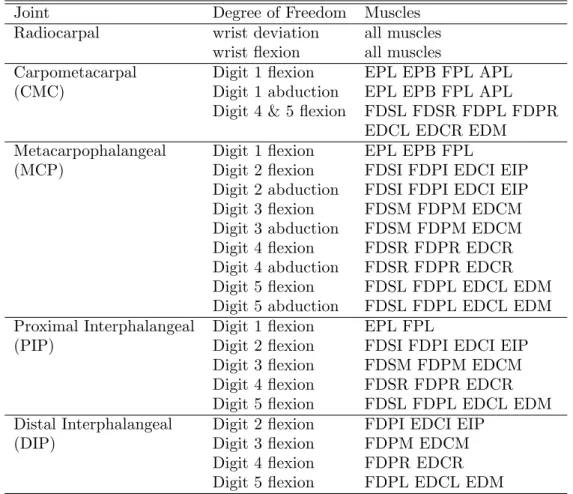
Table 2. The degrees of freedom in the model, and the muscles that cross each one. Joint Degree of Freedom Muscles Radiocarpal wrist deviation all muscles

wrist flexion all muscles

Carpometacarpal Digit 1 flexion EPL EPB FPL APL (CMC) Digit 1 abduction EPL EPB FPL APL

Digit 4 & 5 flexion FDSL FDSR FDPL FDPR EDCL EDCR EDM

Metacarpophalangeal Digit 1 flexion EPL EPB FPL

(MCP) Digit 2 flexion FDSI FDPI EDCI EIP Digit 2 abduction FDSI FDPI EDCI EIP Digit 3 flexion FDSM FDPM EDCM Digit 3 abduction FDSM FDPM EDCM Digit 4 flexion FDSR FDPR EDCR Digit 4 abduction FDSR FDPR EDCR Digit 5 flexion FDSL FDPL EDCL EDM Digit 5 abduction FDSL FDPL EDCL EDM Proximal Interphalangeal Digit 1 flexion EPL FPL

(PIP) Digit 2 flexion FDSI FDPI EDCI EIP Digit 3 flexion FDSM FDPM EDCM Digit 4 flexion FDSR FDPR EDCR Digit 5 flexion FDSL FDPL EDCL EDM Distal Interphalangeal Digit 2 flexion FDPI EDCI EIP

(DIP) Digit 3 flexion FDPM EDCM

Digit 4 flexion FDPR EDCR Digit 5 flexion FDPL EDCL EDM

muscle fibres, the parallel elastic element (PEE) represents the passive properties of muscle fibres and surrounding tissue, and the series elastic element (SEE) represents the tendon and any elastic tissue in the muscle itself that is arranged in series with the muscle fibres.

The state equation for muscle contraction represents the force balance between the elements of the muscle model:

(Factive+fP EE(LCE))cosφ=fSEE(LM −LCEcosφ) (4)

whereLCE is the CE length,LM is the muscle-tendon length,φis the pennation angle, andFactive,

fP EE and fSEE are the forces in CE, PEE and SEE. The equations describing these forces are

included in appendix A of Chadwick et al. (2014). The state variable used for the muscle contraction differential equation iss=LCEcosφ (Chadwick et al. 2014).

2.1.3 Muscle-skeleton Coupling

Moment arms were exported from the OpenSim model for a large number of combinations of joint angles and used to generate polynomial regression models for muscle-tendon length as a function of joint angles (Chadwick et al. 2014).

LM(q) = N X i=1 ci M Y j=1 q_jeij (5)

by the muscle. The moment arm with respect to joint angle k (where 1 ≤ k ≤ M) is obtained by partial differentiation with respect to the kth joint angle (i.e. the ratio between muscle-tendon shortening velocity and joint angular velocity).eij are the polynomial exponents, up to a maximum

of four, andciare the coefficients found by minimizing the error in moment arms and muscle-tendon

length of the polynomial model, relative to the Opensim results.

2.1.4 System Dynamics

If the equations of motion are combined with the muscle dynamics, the model can be described with an implicit first-order differential equation:

f(x,x, u) = 0˙ (6) The state vectorxcontains 94 variables: 23 anglesq, 23 angular velocities ˙q, 24 muscle contraction state variabless, and 24 muscle active states a. The function f has 94 equations, and consists of four parts:

• 23 identities _dtd(x(1 : 23)) = ˙x(1 : 23)

• 23 multibody equations of motion (eq 1)

• 24 muscle activation dynamics equations (eq 3)

• 24 muscle contraction dynamics equations (eq 4)

2.1.5 Implementation

Equations of motion for the model were derived using Autolev (Online Dynamics Inc., Sunnyvale, CA). Muscle dynamics were implemented using custom C code. The dynamic residualsf and the Jacobians are calculated in a Matlab MEX function (Mathworks, Inc., Natick, MA).

2.2 Real-time simulation and numerical stability

Forward dynamic simulation of a musculoskeletal system model involves solving the state trajectory x(t), given an initial statex(0) and controlsuas functions of time and/or state. Due to the implicit formulation of the system equationf, and the fact that all functions used (e.g. the muscle contractile force, etc.) are continually differentiable, we can calculate exact analytical Jacobians ∂f_∂x,∂f_∂x˙ and

∂f

∂u. This allows efficient simulation with an L-stable implicit Rosenbrock method based on the

backwards Euler discretisation:

∆x= ∂f ∂x + 1 h ∂f ∂x˙ −1 ∂f ∂x˙x˙n−f(xn,x˙n, un)− ∂f ∂u(un+1−un) xn+1=xn+ ∆x ˙ xn+1= ∆x h (7)

For the derivation of the above equation see the appendix in (van den Bogert et al. 2011). We ran a test simulation in which the system started in a passive equilibrium state with the humerus set at 50◦ of elevation, the elbow set at 130◦ of flexion, the wrist straight and the fingers at relaxed extension. This upright position was chosen to allow the simulation of American Sign Language postures (see section 2.3).

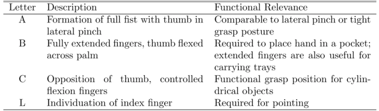
Table 3. Hand postures simulated in this study, that represent the letters A, B, C and L in the American Sign Language Letter Description Functional Relevance

A Formation of full fist with thumb in lateral pinch

Comparable to lateral pinch or tight grasp posture

B Fully extended fingers, thumb flexed across palm

Required to place hand in a pocket; extended fingers are also useful for carrying trays

C Opposition of thumb, controlled flexion fingers

Functional grasp position for cylin-drical objects

L Individuation of index finger Required for pointing

Figure 1. The hand model in the four postures, from left to right: letters A, B, C and L. Top row: anterior view, bottom row: lateral view.

Neural excitations in all muscles were ramped up to reach the maximum (u=1) at t = 0.2s, then kept constant untilt= 1.0s, after which the excitations were set to zero. The simulation was continued untilt= 4.0s.

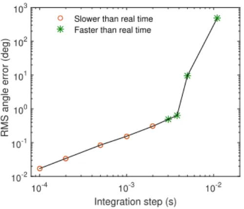
To investigate the accuracy of the implicit method, we ran the same simulation using two solvers: the implicit Rosenbrock method, and the Matlab ode15s solver, an explicit variable-order solver for stiff problems (Shampine L. F. 1997), used with the default tolerance settings. We used a timestep ranging from 0.1msto 10msfor the implicit solver, and recorded the time span of the simulation, and the root mean squared (RMS) error between the angles simulated with the implicit and explicit solvers.

2.3 System stability

The system stability of the model was investigated by linearizing the model in selected active equilibrium states, and judging the local stability from the eigenvalues of the system matrix (van Soest et al. 2003).

The active equilibrium states chosen for this investigation were some of the postures used in the American Sign Language, because the hand-spelling postures of the sign language alphabet bring the fingers into most of their available range of motion (Jerde, T.E., Soechting, J.F. & Flanders 2003). As mentioned before, to achieve these postures, the humerus was set at 50◦ of elevation, and the elbow at 130◦ of flexion, so that the forearm pointed upwards.

Our model does not include contact from finger to finger, so we chose four postures that represent a variety of fine motor skills, but do not require contact: the postures that represent the lettersA, B,C and Lin the American Sign Language (table 3 and figure 1).

Finding the active equilibrium state at each posture was formulated as an optimization problem. We search for the system state x and controls u such that the sum of squared muscle excitations is minimized (min effort) or maximized (max effort), the joint angles match the required posture, and the system is at active equilibrium, i.e. ˙x= 0:

f(x,0, u) = 0 (8)

The max effort condition was included because it results in muscle cocontraction that could increase stability. This constrained optimization problem was solved with SNOPT (Gill et al. 2002).

At active equilibrium, we can linearize the system to obtain the dynamics for small perturbations y:

∂f ∂xy+

∂f

∂x˙y˙= 0 (9)

and judge stability from the system matrixA:

A=− ∂f ∂x˙ −1 ∂f ∂x (10)

If the real parts of all eigenvalues of A are negative, the linear system is stable and thus the nonlinear system is locally stable.

3. Results

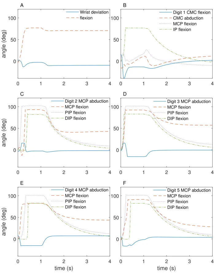
The result of the test simulation is shown in figure 2. Since the initial posture (with the forearm pointing upwards) is an unstable equilibrium, the wrist quickly flexes (the hand drops forward) and stays down even after the excitations have gone back to zero. During maximum excitation, the fingers flex to a fist, and then slowly relax.

The CPU time required for each time step of the implicit solver was 2.94ms on an Intel Xeon E3 processor at 3.2GHz. This means that a time step of 2.94ms or above resulted in faster than real-time performance. For comparison, the ode15s solver required an average stepsize of 0.14ms.

Figure 3 shows the RMS error between the implicit method and ode15s for a range of timesteps used for the implicit simulations. The simulation is numerically stable up to a timestep of 3.80ms, with an error of 0.6◦.

The local stability analysis shows that the model is locally unstable (table 4). The maximum real parts of the eigenvalues of the system matrix are less in the case of maximum effort, but still positive, which means that muscle cocontraction reduces but does not eliminate instability.

As figure 4 shows, muscle cocontraction takes place at the wrist, with co-activation of the main wrist extensors (ECRL, ECRB) and flexors (FCR, FCU). Lack of redundancy in the muscles that control the fingers results in activity of the hand muscles that is mostly the same in the two cases.

0 1 2 3 4

angle (deg)

0 50 100 A Wrist deviation flexion 0 1 2 3 4 0 50 100 B Digit 1 CMC flexion CMC abduction MCP flexion IP flexion 0 1 2 3 4

angle (deg)

0 50 100 C Digit 2 MCP abduction MCP flexion PIP flexion DIP flexion 0 1 2 3 4 0 50 100 D Digit 3 MCP abduction MCP flexion PIP flexion DIP flexion

time (s)

0 1 2 3 4

angle (deg)

0 50 100 E Digit 4 MCP abduction MCP flexion PIP flexion DIP flexion

time (s)

0 1 2 3 4 0 50 100 F Digit 5 MCP abduction MCP flexion PIP flexion DIP flexion

Figure 2. The angles during the 4-second forward simulation. 4. Discussion

The long-term goal of this work is to develop a model of the intact hand that can be implemented in a controller for a prosthesis, allowing natural physiological signals from the user to control the

Integration step (s)

10-4 10-3 10-2

RMS angle error (deg)

10-2 10-1 100 101 102 103

Slower than real time Faster than real time

Figure 3. The error between the implicit method and Matlab’s ode15s vs the timestep. Table 4. The maximum real part of the eigenvalues of the system matrix (MRE) in the active equilibrium states.

MRE (s−1) Letter Min effort Max effort

A 7.58 3.29

B 2.20 1.71

C 3.71 1.98

L 10.60 2.81

terminal device. The aims of this study were to examine the feasibility of this from two perspectives: the ability to simulate the required hand model in real time, and the stability of a hand model controlled by extrinsic muscles only.

For real-time performance, forward dynamic simulation of the musculoskeletal system must take place in real time. This means that the computation time per step in the solver needs to be smaller than the maximum stable step size for the integration. In this case, we found the maximum numerically stable step size to be 3.80ms, and the computation time per step was 2.94ms. This means that real-time simulation of hand motion is possible on the hardware we have available.

The simulated movement resulted in natural looking postures that reproduced the desired inputs. However, for implementation in a real prosthetic device, an important factor will be how close the muscle activations are to real-life muscle activations. Do normal physiological muscle activation patterns produce the same postures? The model described in this study is an extension of published models of the wrist, finger and thumb in which kinematics have been determined from CT images (Buffi et al. 2013), and the force production capabilities have been compared against measured maximum moment curves and endpoint forces (Holzbaur et al. 2005; Saul et al. 2015; Wohlman and Murray 2013). Future work will quantify the differences between measured and simulated muscle activations and kinematics, that arise at least in part from excluding intrinsic muscles.

Another issue that needs to be addressed is computational resources; this work was done on a desktop computer. Because successful implementation for prosthesis control implies the computa-tions would take place on the prosthesis itself, the issue of the computational power available for an embedded system will ultimately need to be addressed. In the case where embedded processors lack sufficient computational power, further reduction of the computational requirements of the model, beyond what we have achieved here, could be explored. For example, the structure of the model could be optimised to reduce the number of states with low time constants, so that the maximum stable step size could be increased.

In terms of model stability, our results show that the model is unstable. One of the reasons for this instability is the simplified nature of the current model. This model consists of extrinsic muscles only for controlling the fingers, and the intrinsic muscles essential to fine control of the hand are not present. The system instability has a time constant of 0.1-0.6 seconds (1/MRE in

0 0.5 1 A Max effort Min effort 0 0.5 1 B Muscle activations 0 0.5 1 C Muscle

ECRLECRBECUFCRFCU PL

FDSLFDSRFDSMFDSI FDPLFDPRFDPMFDPI EDCLEDCREDCMEDCIEDM

EIP _EPLEPBFPLAPL 0

0.5

1 D

Figure 4. The muscle activations for each active equilibrium posture. Panels A, B, C and D show the muscle activations for letters A, B, C and L respectively.

table 4), which is too fast to allow users to accommodate this. It will therefore be necessary to improve the stability of the system to achieve functional prosthesis control.

If one examines the architecture of the hand then instability of a model featuring only extrinsic muscles is not surprising, based on the finger anatomy and the locations of muscle insertions (Fig. 5). The deep flexors and the extensors insert on the distal phalanx, and the superficial flexors insert on the middle phalanx. There is no insertion of extrinsic muscles on the proximal phalanx, leaving the metacarpophalangeal joint uncontrolled in the model; the proximal interphalangeal joint is also under-controlled as it cannot be extended independently.

To address this instability, passive structures representing the complex extensor apparatus (Lei-jnse and Spoor 2012) and other ligaments in the hand that facilitate dexterous control will be added in future work. These structures couple interphalangeal joint rotations and therefore effec-tively reduce the number of DoF that need to be controlled explicitly. This is expected to lead to an increase in the stability of the model.

Furthermore, although our intention was to predict movements based on muscles available in the forearm following hand amputation, the lack of stability means that including intrinsic muscles might be essential. This would increase the number of actuators such that there are no DOF left uncontrolled. Since the activation of those muscles cannot be measured directly from an individual without an intact hand, neural activations of the intrinsics could be predicted from measured activations of the extrinsic muscles based on a mapping established from observation of normally-limbed individuals.

Adding the intrinsic muscles obviously has implications for the performance of the model, and it might be queried whether we could still achieve real time with substantially more muscles. In fact,

Figure 5. The attachments of the deep and superficial muscles of the fingers (index finger shown here). The proximal phalanx does not contain an insertion from extrinsic muscles, leaving it uncontrolled in a model without intrinsics and susceptible to buckling.

preliminary testing for this work indicates that we can add approximately 150 muscle elements to the model, and still achieve real-time performance.

In addition, to implement a real prosthesis controller based on a musculoskeletal model, the model needs to be able to deal with fingertip contact to allow the hand to interact with the environment. These forces could be recorded by force sensors on the prosthesis fingertips and sent to the model. Test simulations we carried out indicate that adding external forces at the fingertips to the model results in an increase in computation time of 0.08%. Consequently this will not be an impediment to real-time simulation.

Finally, although our method relies on using EMG signals as inputs to the model, in fact any neural signal, including that from peripheral nerves, can be used. Integrating with peripheral nerves has the advantage that the control signals to the intrinsic muscles can be recorded, even though the muscles themselves are not present. This would solve the problem of mapping the activation of the intrinsics from the extrinsics. Moreover, integration with the nervous system would allow us to not only measure movement intent, but give feedback through stimulation of the nerve (Micera et al. 2010). This feedback may take the form of proprioception through the use of virtual muscle spindles and Golgi tendon organs. Force sensors at the fingertips could also provide touch feedback and further enhance the level of control provided to users of prosthetic devices (Tan et al. 2014).

5. Conclusion

We have shown that a simplified biomechanical model of the human hand that has sufficient complexity to represent a range of postures can be made to run in real time using an implicit solver. Numerical stability of the forward dynamic simulation was maintained up to a solver step size of 3.8ms, allowing real-time simulation on desktop hardware. The model showed system instability in the postures tested, even with high values of cocontraction, due to the lack of stabilising structures such as intrinsic muscles. This implies the need for additional stabilising measures to allow use of the model for prosthesis control.

Funding

The authors would like to acknowledge funding from the National Institutes of Health (R01-EB011615).

References

Biddiss E, Beaton D, Chau T. 2007. Consumer design priorities for upper limb prosthetics. Disability and rehabilitation Assistive technology. 2(6):346–357.

Biddiss E, Chau T. 2007. Upper-limb prosthetics: critical factors in device abandonment. American journal of physical medicine & rehabilitation / Association of Academic Physiatrists. 86(12):977–87.

Buffi JH, Crisco JJ, Murray WM. 2013. A method for defining carpometacarpal joint kinematics from three-dimensional rotations of the metacarpal bones captured in vivo using computed tomography. Journal of Biomechanics. 46:2104–2108.

Buffi JH, Sancho Bru JL, Crisco JJ, Murray WM. 2014. Evaluation of Hand Motion Capture Protocol Using Static Computed Tomography Images: Application to an Instrumented Glove. Journal of Biomechanical Engineering. 136(12):124501.

Chadwick E, Blana D, Kirsch R, van den Bogert A. 2014. Real-Time Simulation of Three-Dimensional Shoulder Girdle and Arm Dynamics. IEEE Transactions on Biomedical Engineering. 61(7):1947–1956. Childress, D & Weir R. 2003. Control of Limb Prostheses. In: DG Smith JMJB, editor. Atlas of amputations

and limb deficiencies. American Academy of Orthopaedic Surgeons, Rosemont, IL.

Cipriani C, Segil JL, Birdwell JA, Ff RF. 2014. Dexterous Control of a Prosthetic Hand Using FineWire Intramuscular Electrodes in Targeted Extrinsic Muscles. IEEE Trans Neural Syst Rehabil Eng. 22(4):828– 836.

Delp SL, Anderson FC, Arnold AS, Loan P, Habib A, John CT, Guendelman E, Thelen DG. 2007. OpenSim: open-source software to create and analyze dynamic simulations of movement. IEEE Transactions on Biomedical Engineering. 54(11):1940–50.

Gill PE, Murray W, Saunders MA. 2002. SNOPT: An SQP Algorithm for Large-Scale Constrained Opti-mization. SIAM Journal on OptiOpti-mization.

Hargrove LJ, Lock Ba, Simon AM. 2013. Pattern recognition control outperforms conventional myoelectric control in upper limb patients with targeted muscle reinnervation. Proceedings of the Annual International Conference of the IEEE Engineering in Medicine and Biology Society, EMBS:1599–1602.

He J, Levine W, Loeb G. 1991. Feedback gains for correcting small perturbations to standing posture. IEEE Transactions on Automatic Control. 36(3):322–332.

Holzbaur KRS, Murray WM, Delp SL. 2005. A Model of the Upper Extremity for Simulating Musculoskeletal Surgery and Analyzing Neuromuscular Control. Annals of Biomedical Engineering. 33(6):829–840. Jerde, TE, Soechting, JF & Flanders M. 2003. Biological constraints simplify the recognition of hand shapes.

Ieee Transactions on Biomedical Engineering. 50:265–269.

Jiang N, Dosen S, Muller KR, Farina D. 2012. Myoelectric Control of Artificial Limbs - Is There a Need to Change Focus? [In the Spotlight]. IEEE Signal Processing Magazine. 29(5):152–150.

Leijnse JNaL, Spoor CW. 2012. Reverse engineering finger extensor apparatus morphology from measured coupled interphalangeal joint angle trajectories - a generic 2D kinematic model. Journal of Biomechanics. 45(3):569–578.

Micera S, Carpaneto J, Raspopovic S. 2010. Control of hand prostheses using peripheral information. IEEE Reviews in Biomedical Engineering. 3:48–68.

Muzumdar A. 2004. Powered Upper Limb Prostheses: Control, Implementation and Clinical Application. Springer.

Pylatiuk C, Schulz S, D¨oderlein L. 2007. Results of an Internet survey of myoelectric prosthetic hand users. Prosthetics and orthotics international. 31(4):362–370.

Sachdeva P, Sueda S, Bradley S, Fain M, Pai DK. 2015. Biomechanical simulation and control of hands and tendinous systems. ACM Transactions on Graphics. 34(4):42:1–42:10.

Saul KR, Hu X, Goehler CM, Vidt ME, Daly M, Velisar A, Murray WM. 2015. Benchmarking of dynamic simulation predictions in two software platforms using an upper limb musculoskeletal model. Computer methods in biomechanics and biomedical engineering. 18(13):1445–58.

Schutte L. 1992. Using musculoskeletal models to explore strategies for improving performance in electrical stimulationinduced leg cycle ergometry. [dissertation]. Stanford.

Shampine L F RMW. 1997. The MATLAB ODE Suite. SIAM Journal on Scientific Computing. 18:1–22. Smith LH, Kuiken Ta, Hargrove LJ. 2014. Real-time simultaneous and proportional myoelectric control

using intramuscular EMG. Journal of Neural Engineering. 11(6):066013.

Sueda S, Kaufman A, Pai DK. 2008. Musculotendon simulation for hand animation. ACM Transactions on Graphics. 27(3):1-8.

Tan DW, Schiefer MA, Keith MW, Anderson JR, Tyler J, Tyler DJ. 2014. A neural interface provides long-term stable natural touch perception. Science Translational Medicine. Vol. 6, Issue 257, pp. 257ra138 van den Bogert AJ, Blana D, Heinrich D. 2011. Implicit methods for efficient musculoskeletal simulation

and optimal control. Procedia IUTAM. 2:297–316.

van Soest aJ, Haenen WP, Rozendaal La. 2003. Stability of bipedal stance: the contribution of cocontraction and spindle feedback. Biological cybernetics. 88(4):293–301.

Waryck B. 2011. Comparison of two myoelectric multi-articulating prosthetic hands. In: Proceedings of the 2011 MyoElectric Controls/Powered Prosthetics Symposium; Fredericton, New Brunswick, Canada. Wohlman SJ, Murray WM. 2013. Bridging the gap between cadaveric and in vivo experiments: A

biome-chanical model evaluating thumb-tip endpoint forces. Journal of Biomechanics. 46(5):1014–1020.

Young AJ, Smith LH, Rouse EJ, Hargrove LJ. 2013. Classification of Simultaneous Movements Using Surface EMG Pattern Recognition. IEEE Transactions on Biomedical Engineering. 60(5):1250–1258. Available from: http://ieeexplore.ieee.org/document/6377275/.