Pattern Classification in Imbalanced Data-Sets
Marcia Amstelvina Saul1 and Shahin Rostami2
Faculty of Science & Technology, Bournemouth University, Bournemouth, BH12 5BB, United Kingdom
1
2
WWW home page:https://research.bournemouth.ac.uk/project/ciri/
Abstract. Class imbalance is a common challenge when dealing with pattern classification of real-world medical data-sets. An effective counter-measure typically used is a method known as re-sampling. In this paper we implement an ANN with different re-sampling techniques to subse-quently compare and evaluate the performances. Re-sampling strategies included a control, under-sampling, over-sampling, and a combination of the two. We found that over-sampling and the combination of under- and over-sampling both led to a significantly superior classifier performance compared to under-sampling only in correctly predicting labelled classes. Keywords: machine learning, imbalanced data, over-sampling, under-sampling
1
Introduction
There is an increasing interest in the application of machine learning in provid-ing assistance to diagnosticians whom may otherwise be uncertain of a prognosis [26]. Previous research into predictive measures have found that pattern detec-tions can be extracted from medical tracings and medical imaging, such as; identification of diabetic retinopathy [23], cancerous cells in dermatology [11] and identifying brain tumours in MRI scans [29]. Classification models which take into account previous medical cases could reduce the time taken to arrive at a prognosis, and even suggest possible onset of a disease to treat it before the harmful symptoms manifest [26]. Artificial neural networks (ANNs) have previ-ously improved the performance of potentially out-of-date and ungeneralizable indexes or heuristics still used in the health-care industry [26] by allowing clini-cians to make more informed decisions about their diagnosis. As such, machine learning is a vital tool in bridging the gaps of missing information within these tests to increase the validity and accuracy of the suggested prognosis. In addi-tion, successful implementation of such an ANN will also reduce the risk of the disease worsening and the corresponding financial implications. These workings ultimately lead towards one major outcome, that is overall patient satisfaction [26].
In the health-care industry, there is often the challenge of class imbalance within the data-set i.e. when classes are significantly over/under represented, particularly when concerning rare diseases or abnormalities. For example, con-sider a scenario where smallpox has become re-apparent and clinicians must quickly differentiate between spots symptomatic of chickenpox and those of smallpox to hasten eradication. The engineers may notice that out of the 1,000 case files, only 10 were reported of smallpox. If the engineers feed this data into a neural network, what they would find is that approximately 990 predicted output values would successfully estimate very close to the target output values. This suggests that the network model has 99% accuracy, however this is not nec-essarily a useful indication of its performance. Whilst it would indeed have 99% accuracy for correctly predicting chickenpox, they would also have 0.01% accu-racy for correctly predicting smallpox (if the model could predict for smallpox at all). This means that the model overall has poor performance considering that they have built the model to specifically detect smallpox. This is an example of the class imbalance problem, which is typically addressed during pre-processing and manipulation of the data-set prior to ANN training.
The remainder of the paper is organised as follows: In Section 2 the data-set and approaches considered for comparison are discussed, followed by Section 3 which lists and discusses the numerical results complete with a statistical analysis. The paper is then concluded in Section 4 and 5 with recommendations for future research directions.
2
Methods
The data used in the experiments of this paper was obtained from the UCI Machine Learning Repository [7] and contains cardiotocography measurements. Data acquisition and analyses were carried out by [1], presenting a data-set with 23 attributes and 2,126 samples for each attribute (extracted from real-world consenting participants). These attributes include 21 input features and 2 possible output classification criteria to be utilised separately as 3-class or 10-class experiments. The study [1] authors state that the output 10-classes in both criteria were labelled and substantiated by expert obstetricians. This paper uses the 3-class output criteria relating to the detection of foetal states: 'Normal',
'Suspect', and 'Pathologic' from the cardiotocograms. Thus, the preliminary
network architecture incorporated 21 input nodes and 3 output nodes.
In order to solve this pattern classification problem, the first step was to address the data-set itself and its suitability for building classification models upon. The data-set source study on SisPorto 2.0, an automated cardiotocogram analysis system, is a performance test on a wide-scale evaluation. The system was tested on over 6,000 pregnancies across 14 centres in Europe and Australia producing an extent of generalisation, or domain representation, provided analy-sis is conducted on the tested demographics. In addition, tracings from the foetal heart rate (FHR), including baseline, accelerations, deceleration, and variability, were subject to Cohen's kappa coefficient testing. Whereby the clinicians
over-all proportions gave “fair-to-good” agreements of the results [4]. The authors also found a 100% sensitivity and 99% specificity rating for their predictions in neonatal abnormalities [4]. These findings therefore propose a healthy quality of data for building a classification model.
The subsequent and focal issue to be addressed prior to classification was the imbalance of class frequencies. Whilst the experiment will implement different techniques to balancing the classes, the goal across all techniques is to obtain a 1:1:1 ratio. Four different experiments were conducted for balancing classes: over-sampling towards the majority class frequency, under-sampling towards the minority class frequency, a combination of over- and under-sampling towards a sufficiently representative sample size and a benchmark model with no re-sampling to allow for a control experiment.
The rule of thumb when choosing the number of hidden neurons is typically between the number of inputs and the number of outputs [13]. Similarly, for low-scale data-sets, one or two hidden layers are sufficient. The ANN classifier was defined by employing optimiser and loss function algorithms for the learning phase. The Adaptive Subgradient Method, oradagrad, is an optimisation func-tion which has shown to accommodate for different measurement types across the input features [8]. Accompanied by the loss function often used for handling multi-class problems, Categorical Cross-Entropy. Following the implementation and training of the classifiers, performance evaluation measures were applied to test the quality of the predictions made. The evaluation techniques used were the receiver operator characteristic with area under curve (ROC-AUC) as literature suggests its suitability with medical data [14, 2, 22], and the f1-score which repre-sents a harmonic mean between precision and recall measures. Each performance evaluation was computed from a confusion matrix and macro-averaged. The final stage of the experiment was to apply statistical testing to derive the presence of a significant difference between the performances of the trained classifiers across re-sampling techniques.
3
Numerical Results
3.1 Experimental Set-Up
The algorithms employed by this experiment were implemented using the Python 2.7 programming language, which leveraged the Keras (https://keras.io/) neural networks API running on top of the TensorFlow (https://www.tensorflow.org/) machine learning framework. All experiments were conducted within identical Docker containers to facilitate an isolated and reproducible research environ-ment.
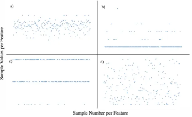
Pre-Processing of Data-Set On extraction from the UCI Machine Learning Repository, the first noticeable property of the raw data-set was that each input attribute had been measured on different scales during analysis on SisPorto 2.0. Fig. 1 illustrates the distribution of 4 input attributes and the extremities
in scaling variance. Accordingly, a standardisation procedure was applied to the data-set as a whole. The data-set was divided into training and testing subsets, using the conventional division of 70% training and 30% testing [13]. Administering this division prior to re-sampling ensures that the testing data is untouched to provide pure values when testing the classifier model.
Fig. 1.Four features represented as scatter-plot; a) Feature: UC, b) Feature: Nzeros, c) Feature: Variance, d) Feature: Width. Extracted from the 'Suspect'data-set prior to pre-processing. Illustrates the complexity of feature measurements and necessity for standardisation of data.
The output nodes of'Normal','Suspect', and'Pathologic'foetal states com-prise of 1,655, 295, and 176 samples per feature respectively. The over-sampling only experiment obtained the 1:1:1 ratio by re-sampling so each class was of 1,655 elements each. Conversely, the under-sampling only experiment was re-sampled so each class was of 176 elements each. The combination of over- and under-sampling techniques was where provisions were made in order to deter-mine a representative class size. To derive the class sizes, ANOVA fixed-effects tests were used with a pre-determined power (1-β, where theβ-value represents Type II error), alpha (α, Type I error), and effect size (f). Clinically based stud-ies suggest α-values and (1-β)-values of at least 0.05 and 0.80 respectively as standard for optimal testing [16]. Subsequently, f was determined using a type of effect size known as the risk ratio [12], recommended for binary-type classes [27]. Typically, effect sizes are calculated as a statistical measure between two classes and the number of classes in this experiment exceeded this limitation. Previous studies [3, 20] suggest that to overcome this problem, it is necessary to transfer the statistical inference by testing between the two outermost classes, i.e.'Normal'(C1) and'Pathologic'(C3). Therefore, the effect size (1) was calcu-lated, wheren is the number of total elements across the classes. The G*Power 3.1 [9] software application was used to execute the ANOVA fixed-effects test and it was calculated that 861 elements per class were required as an optimal class size given the prior parameters.
RiskRatio= C1/n C3/n =
176/2126
1655/2126 = 0.106 (1)
Re-sampling of the data-set followed the determination of target class sizes. Over-sampling was applied by incorporating a variant of the synthetic data generation technique, SMOTE [5], known as SVM (Support Vector Machine) SMOTE. This variant of SMOTE generates new synthetic data using SVMs to predict new unknown elements at the borderline of the minority classes [17]. This method is capable of substantiating the decision boundary for the classi-fier and also expand minority classes which occur in the data space of majority class elements [17]. The intuition for the SMOTE technique is to generate new data elements in feature space as opposed to data space to reduce over-fitting. Under-sampling was applied using NearMiss-2 [28, 30], a technique which em-ploys a clustering k-NN (nearest neighbour) algorithm to select elements from the majority class which has the smallest averaged distance from thekfurthest minority elements. NearMiss is a controlled under-sampling method, which en-abled the experiment to define the number of elements for each under-sampled class. In addition, NearMiss-2 has been found to perform optimally out of all the NearMiss variants [28]. The combination of over- and under-sampling employed SVM SMOTE on the 'Suspect'and 'Pathologic'classes whilst NearMiss-2 was be employed for the'Normal'class.
Network Architecture and Parameter Configuration The ANN topology
consisted of 21 input nodes and 3 output nodes across all re-sampling experi-ments. There were 2 hidden layers implemented for the classifier model, with 21 hidden neurons integrated in each layer. Each hidden layer applied the Rectified Linear Unit (ReLU) activation function. The data fed into the ANN for train-ing corresponds to the class sizes which had been established previously. The dimensions of the input data matrix consisted of 4,965 by 21 for over-sampling only, 528 by 21 for sampling only, and 2,583 by 21 for over- and under-sampling. The control experiment had no re-sampling, and therefore consisted of the original 2,126 by 21 matrix. Each sample was fed into the ANN individually and the entire data-set was used for training the ANN iteratively for a maximum of 500 epochs.
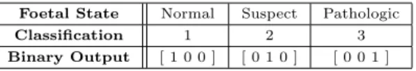
To ensure accurate model predictions, it was essential that the output layer was a binary representation of the foetal state classes (Table 1). This is due to the fact that the original raw data-set classifies the foetal states by assigning'1',
'2', and '3' to 'Normal', 'Suspect', and 'Pathologic' respectively. It would be
difficult to confirm which class the ANN was attempting to predict if the values obtained were continuous (i.e. verifying a predicted output of 2.5 towards either 2 or 3). In addition, a typical output layer activation function (such as the sigmoid activation function which were used in these experiments) squashes retrieving values between 0 and 1, then activates if the value exceeded 0.5. Therefore, less dubious translations of model predictions to class predictions could be made when binary representations of the output were implemented.
Foetal State Normal Suspect Pathologic
Classification 1 2 3
Binary Output [ 1 0 0 ] [ 0 1 0 ] [ 0 0 1 ]
Table 1. Binary output illustrated the activation of only one neuron in the output layer at a time.
During training, over-fitting preventative strategies were incorporated by setting a neuron dropout of 0.25 between layers (sets a percentage of neuronal output to 0) and neutralised the high epoch of 500 with an early stopping cri-terion [21]. Early stopping allowed the iterations of training to stop if the loss function does not improve for a specified amount of consecutive iterations, in-creasing robustness of the network.
Statistical Analysis Once the classifier model was built and trained, the ROC-AUC and f1-score performance evaluations were calculated. In order to deter-mine the presence of a significant difference between the re-sampling strategies, statistical analysis was conducted on these performance evaluations.
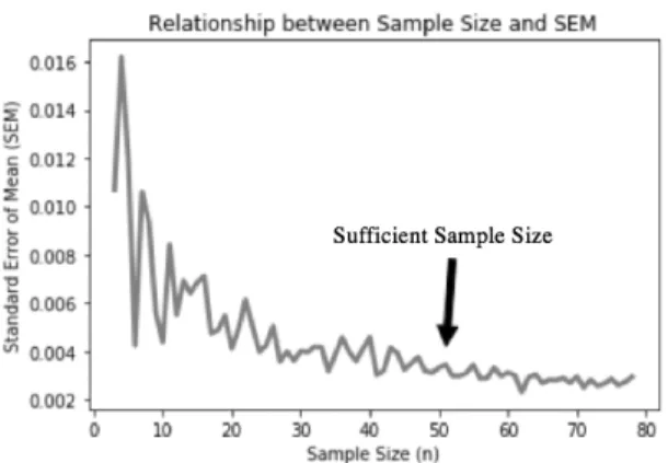
Firstly, the number of times each experiment was ran to determine the sam-ple size for analysis was obtained by extracting the standard error of the mean (SEM) per number of trials. The number of times an experiment was trialled was grouped into an overall sample size. The SEM of the performance evalua-tion values were extracted from a starting point of 3 samples (i.e. running the experiment 3 times) and continued towards 80 samples. Fig. 2 illustrates how the SEM changes with sample size. It could be observed that past 50 samples the SEM curve began to plateau and a larger sample size would not entail a notably greater effect worthy of additional trials when it came to the analysis.
Having established the sample size, the distribution normality of the per-formance evaluation data for each experiment was tested. The p-values from D'Agostino and Pearson's [6, 18] test for normality was extracted for each class from measures of precision, recall and ROC-AUC (a macro-average of the f1-score as the harmonic mean of precision and recall was computed and therefore these distributions were tested for normality). Using anα-value of 0.001, a collec-tion of both normally and non-normally distributed data was found. The overall consensus, however, was that a non-parametric test was required to measure the statistical significance between the four experiments. This is because the macro-average of both the f1-score and the ROC-AUC were used as the components of the samples under statistical analysis. There were no two performance evalua-tion classes which contained purely normally or non-normally distributed data and a parametric test is bound in its ability to account for the non-parametric details of certain classes. Therefore, the non-parametric Wilcoxon signed-rank test (tests the medians of “two paired measurements made on identifiable pop-ulation” [10]) was implemented to test for a significant difference between the performance evaluation outcomes of each re-sampling experiment.
Fig. 2. The standard error of mean was measured for each number of times the ex-periment was run to determine an appropriate sample size for statistical analysis. The SEM data was extracted from the control group experiment.
3.2 Experimental Results
Performance evaluation measures were obtained by computing the confusion matrix for each experiment (Fig. 3). Hereafter, 'combi-sampling' refers to the over- and under-sampling experiment.
Correctly labelled samples (true positives) are represented diagonally in the boxes where the actual output class meets its corresponding predicted output class [24], i.e. 'Normal'-'Normal'. Whilst the off-diagonal values in the matrix represent mislabelled samples [24] (true negatives, false positives and false neg-atives). Throughout the experimental trials, over-sampling and combi-sampling exhibited consistent performance in the outcomes of the true positive values of the confusion matrix. For each class, both experiments held between 0.70 and 0.99 for each class true positive rate and low values of mislabelled samples over the 50 trials. On the other hand, there were fluctuating outcomes of correctly la-belled samples for the control and under-sampling. Generally, both experiments had higher levels of mislabelled samples and were unable to predict all classes to the level exhibited by over-sampling and combi-sampling. Under-sampling ei-ther predicted one class well and poorly for the remaining two, or poorly for all classes. Control, as expected with no re-sampling, predicted only class'Normal' well, with occasional good prediction for either one of the remaining classes but never all three classes.
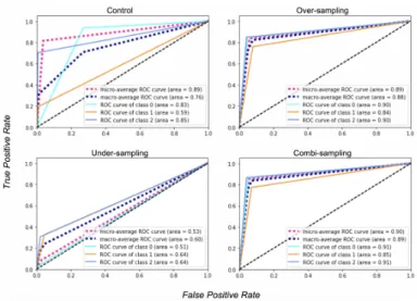
From the confusion matrix, the ROC-AUC values for each class and its corre-sponding macro-average were computed for testing of the classifier performance. The ROC curve is defined as illustrating an excellent performance of a model when its area (AUC) is 1.00 [25]. In other words, the curve peaks at the begin-ning of the plot and maintains the inflated y-values (true positive rate) along x (false positive rate). Fig. 4 portrays the ROC curves and AUC values for each re-sampling experiment.
Fig. 3.Confusion matrices extracted from the last trial of each re-sampling experiment.
Fig. 4. Receiver operator characteristic (ROC) curves extracted from the last trial of each re-sampling experiment. Area under curve (AUC) values for each class and averaged values are indicated in the legend box of each plot.
All re-sampling techniques reduced the distances of the ROC curves for each class from each other, illustrating the 1:1:1 ratio across 'Normal', 'Suspect', and 'Pathologic' classes. Similarly to the results of the confusion matrix, the ROC-AUC metrics for over-sampling and combi-sampling were alike in shape and showed indications of correctly labelled classes by the classifier model. Also similarly, under-sampling was unable to perform as well as over-sampling and combi-sampling.
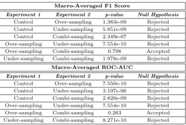
Table 2 shows the results of the statistical analysis made using the Wilcoxon signed-rank test for a difference between the performance evaluations of each re-sampling technique. The null hypothesis (there was no difference between the medians of the corresponding two measurements) was tested. Each test statistic was calculated at a 95% confidence level i.e.α-value = 0.05.
Statistical significance between each re-sampling experiment was determined by whether the null hypothesis was accepted or rejected for both evaluation metrics. All re-sampling experiments exhibited a significantly different classifier model performance to the control. This result drives the need for re-sampling when dealing with imbalanced data-sets for pattern classification problems using ANNs. Over-sampling and combi-sampling both presented significant differences in performance with under-sampling, whilst having no significant difference in performance with each other. This finding was congruous with the illustrations in Fig.3 and Fig.4 of the confusion matrices and ROC curves respectively.
Macro-Averaged F1 Score
Experiment 1 Experiment 2 p-value Null Hypothesis Control Over-sampling 1.383e-09 Rejected Control Under-sampling 5.851e-09 Rejected Control Combi-sampling 2.349e-07 Rejected Over-sampling Under-sampling 7.554e-10 Rejected Over-sampling Combi-sampling 0.798 Accepted Under-sampling Combi-sampling 1.978e-09 Rejected
Macro-Averaged ROC-AUC
Experiment 1 Experiment 2 p-value Null Hypothesis Control Over-sampling 7.550e-10 Rejected Control Under-sampling 3.197e-06 Rejected Control Combi-sampling 2.820e-09 Rejected Over-sampling Under-sampling 7.554e-10 Rejected Over-sampling Combi-sampling 0.263 Accepted Under-sampling Combi-sampling 8.271e-10 Rejected
Table 2. Results of the Wilcoxon signed-rank test between every re-sampling exper-iment from the macro-averaged f1 score and ROC-AUC. The null hypothesis of no difference between experiments is rejected if the p-value is less thanα-value = 0.05.
4
Discussion
The experimental design of combi-sampling was incorporated as a proposition to address the distinctive frequency discrepancy between classes. By solely in-corporating under-sampling, there is a risk of losing essential data in more than one feature of the data-set. On the other hand, pure over-sampling poses a risk of over-fitting the classifier model. Due to the use of early stopping and neuron dropout methods, there could be some exoneration of sampling from over-fitting the classifier model. However, it appeared from the statistical analyses that the under-sampling methods did indeed manage to lose essential data points in attempting to represent a complex data-set. By observing the methodology used in this paper for extracting a sufficient sample size for the combi-sampling experiment, it could be seen that the statistically minimum sample size required to be representative of the data-set was 861 elements per class. This meant that in the under-sampling experiment, the classes had a critically insufficient size of 176 elements per class. In addition, considering the existing limitation of ob-taining a comprehensively generalizable cardiotocography data-set that includes the statistics of every pregnant woman, it would be favourable to build upon existing data and maintain the existing essential elements with over-sampling rather than lessen the data with under-sampling.
Although over-sampling and combi-sampling produced satisfactory perfor-mance evaluation scores, there is still room for improvement (i.e. bringing the AUC value closer to 1.00). Real-life applications of machine learning in health-care would focus on this optimisation of state predictions to enhance preventative techniques. Therefore, some further work on the extension of this paper is re-quired. Firstly, with the matter of classifier performance in general, the'Suspect' data-set had perhaps been difficult to class because it contained aspects of data which could fall in either the 'Normal'data-set or the'Pathologic'data-set. In other words, there were overlapping data-instances either already existent in the original data-set or introduced via the re-sampling strategies [19]. By comparing this paper to the results of an alternative machine learning technique (such as fuzzy logic systems which have been shown to work well with data-sets contain-ing overlappcontain-ing categories [15]), we may be able to determine if an alternative technique is able to provide a superior predictive performance. In addition, some further work could be done in establishing that over-fitting was indeed avoided within the over-sampling and combi-sampling experiments. Lastly, a larger data-set could be implemented to establish a more detailed view by introducing a larger set of unseen testing data, or an experiment incorporating and evaluating the effect of different ANN classifiers (i.e. variant network topologies, optimisers or loss-functions).
5
Conclusion
In this paper, the performance evaluation of an ANN classifier in predicting foetal states from cardiotocography measurements using different re-sampling
techniques was presented. The main findings concluded that over-sampling and combi-sampling were able to reasonably predict all classes 'Normal', 'Suspect' and'Pathologic'. Over-sampling and combi-sampling maintained a level of per-formance with each other (no significant differences) and accomplished signifi-cantly more accurate results than under-sampling, whose performance allowed the classifier to only sufficiently predict only one class at a time, if at all.
Furthermore, a significant difference between all re-sampling techniques and the control was found, reiterating the pivotal role of re-sampling of data-sets when dealing with class imbalances. The adverse effects of no re-sampling is additionally illustrated by the control ROC-AUC curve (Fig. 4), whereby an inconsistency in performance exists across classes. By balancing class frequencies, it eradicated means of false accuracy exhibited in the control and significantly improved the performance of an ANN classifier model in order to assess the differences in re-sampling techniques for a pattern recognition problems.
References
1. Ayres-DeCampos, D., Bernardes, J., Garrido, A., MarquesDeS, J., PereiraLeite, L.: Sisporto 2.0: A program for automated analysis of cardiotocograms. The Journal of MaternalFetal Medicine9, 311318 (2000)
2. Bradley, A.P.: The use of the area under the roc curve in the evaluation of machine learning algorithms. Pattern Recognition30(7), 11451159 (1997). DOI 10.1016/ s0031-3203(96)00142-2
3. Brooks, G.P., Johanson, G.A.: Sample size considerations for multiple comparison procedures in anova. Journal of Modern Applied Statistical Methods10(1), 97109 (2011). DOI 10.22237/jmasm/1304222940
4. de Campos, D.A.: The sisporto automated analysis
5. Chawla, N., Bowyer, K., Hall, L., Kegelmeyer, W.P.: Smote: Synthetic minority over-sampling technique. Journal of Artificial Intelligence Research 16 p. 321357 (2002)
6. Dagostino, R.B.: An omnibus test of normality for moderate and large size samples. Biometrika58(2), 341 (1971). DOI 10.2307/2334522
7. Database, U.M.L.: Cardiotocography data set (2010). URL https://archive.ics.uci. edu/ml/datasets/cardiotocography
8. Duchi, J., Hazan, E., Singer, Y.: Adaptive subgradient methods for online learning and stochastic optimization. Journal of Machine Learning Research 12 p. 21212159 (2011)
9. Dsseldorf, H.H.U.: G*power. URL http://www.gpower.hhu.de/en.html
10. Ennos, A.R., Johnson, M.: Statistical and data handling skills in biology. Pearson Education (2017)
11. Esteva, A., Kuprel, B., Novoa, R., Ko, J., Swetter, S., Blau, H., Thrun, S.: Dermatologist-level classification of skin cancer with deep neural networks. Nature 542(7639), 115–118 (2017)
12. Gigerenzer, G.: Helping doctors and patients make sense of health statistics. Simply Rational p. 2193 (2015). DOI 10.1093/acprof:oso/9780199390076.003.0005 13. Heaton, J.: Introduction to neural networks with Java. Heaton Research (2009) 14. Huang, J., Ling, C.: Using auc and accuracy in evaluating learning algorithms.
IEEE Transactions on Knowledge and Data Engineering 17(3), 299310 (2005). DOI 10.1109/tkde.2005.50
15. Ishibuchi, H., Nakaskima, T.: Improving the performance of fuzzy classifier systems for pattern classification problems with continuous attributes. IEEE Transactions on Industrial Electronics46(6), 10571068 (1999). DOI 10.1109/41.807986 16. Kim, H.Y.: Statistical notes for clinical researchers: Type i and type ii errors in
statistical decision. Restorative Dentistry & Endodontics40(3), 249 (2015). DOI 10.5395/rde.2015.40.3.249
17. Nguyen, H.M., Cooper, E.W., Kamei, K.: Borderline over-sampling for imbalanced data classification. International Journal of Knowledge Engineering and Soft Data Paradigms3(1), 4 (2011). DOI 10.1504/ijkesdp.2011.039875
18. Pearson, E.S., Dagostino, R.B., Bowman, K.O.: Tests for departure from normality: Comparison of powers. Biometrika64(2), 231246 (1977). DOI 10.1093/biomet/ 64.2.231
19. Prati, R.C., Batista, G.E.A.P.A., Monard, M.C.: Class imbalances versus class overlapping: An analysis of a learning system behavior. MICAI 2004: Advances in Artificial Intelligence Lecture Notes in Computer Science p. 312321 (2004). DOI 10.1007/978-3-540-24694-7 32
20. Preacher, K.J., Rucker, D.D., Maccallum, R.C., Nicewander, W.A.: Use of the extreme groups approach: A critical reexamination and new recommendations. Psychological Methods10(2), 178192 (2005). DOI 10.1037/1082-989x.10.2.178 21. Prechelt, L.: Early stopping but when? Neural Networks: Tricks of the Trade
7700(2012). DOI https://doi.org/10.1007/978-3-642-35289-8 5
22. Provost, F., Fawcett, T., Kohavi, R.: The case against accuracy estimation for com-paring induction algorithms. Proceedings of the Fifteenth International Conference on Machine Learning (1998)
23. Saha, R., Chowdhury, A.R., Banerjee, S.: Diabetic retinopathy related lesions de-tection and classification using machine learning technology. Artificial Intelligence and Soft Computing Lecture Notes in Computer Science p. 734745 (2016). DOI 10.1007/978-3-319-39384-1 65
24. Scikit-Learn: Confusion matrix. URL http://scikit-learn.org/stable/auto examples/model selection/plot confusion matrix.html
25. Tape, T.: The area under an roc curve. URL http://gim.unmc.edu/dxtests/roc3. htm
26. Thatcher, L.: The benefits of machine learning in healthcare (2017). URL https: //healthcare.ai/the-benefits-of-machine-learning-in-healthcare
27. University, P.S.: Power and sample size determination for testing a population mean. URL https://onlinecourses.science.psu.edu/stat500/node/46
28. Yen, S.J., Lee, Y.S.: Cluster-based under-sampling approaches for imbalanced data distributions. Expert Systems with Applications 36(3), 57185727 (2009). DOI 10.1016/j.eswa.2008.06.108
29. Zacharaki, E.I., Wang, S., Chawla, S., Yoo, D.S., Wolf, R., Melhem, E.R., Da-vatzikos, C.: Classification of brain tumor type and grade using mri texture and shape in a machine learning scheme. Magnetic Resonance in Medicine 62(6), 16091618 (2009). DOI 10.1002/mrm.22147
30. Zhang, J., Mani, I.: knn approach to unbalanced data distributions: A case study involving information extraction. Workshop on Learning from Imbalanced Datasets II (2003)