Algorithmic advances in learning from large dimensional
matrices and scientific data
A DISSERTATION
SUBMITTED TO THE FACULTY OF THE GRADUATE SCHOOL OF THE UNIVERSITY OF MINNESOTA
BY
Shashanka Ubaru
IN PARTIAL FULFILLMENT OF THE REQUIREMENTS FOR THE DEGREE OF
DOCTOR OF PHILOSOPHY
Yousef Saad
Acknowledgements
This thesis was accomplished with the help and support of many amazing people, who I would like to wholeheartedly thank.
Firstly, I have to thank my PhD advisor,Prof. Yousef Saad. Without his guidance, help and support, this thesis work would not have been possible. I have learned a lot from him, and his knowledge, dedication, and strive for excellence have inspired me greatly. I am deeply indebted to him for his teachings, support and directions, and for giving me the freedom to pursue my varied interests with him and other collabora-tors. I am very fortunate to have worked with and learned from such an extraordinary academic.
Secondly, I wish to thankProf. Arya Mazumdar, who co-advised my Master’s thesis and guided me in many of the projects which are part of this thesis. He helped me explore a new direction of research in applications of coding theory. His hard-work and dedication to research have been great motivations for me.
Next, I want to thank Kristofer Bouchard, who has mentored me for the past two years on many projects related to ML for science, which are also part of this thesis. I also should thank Kesheng Wu, who along with Kris, hosted and mentored me for two summers at Berkeley Lab. I have to also thank Abd-Krim Seghouane, who has guided me in many projects and hosted me at Melbourne last summer. All three of them have helped me and supported me immensely in accomplishing this thesis.
I am grateful to the members of my dissertation committee, Prof. Daniel Boley, Prof. George Karypis, and Prof. Georgios Giannakis, who were very kind to agree to be on the advisory board. I would like to especially acknowledge Prof. Boley here, who served as a member of my Masters’ thesis, PhD qualifier, thesis proposal, and defense committees. He has always been very gracious with his invaluable advises to me.
sors and researchers over the years. I want to thank my collaborators; senior professors: Prof. Alexender Barg, Prof. James Chellikowsky, Prof. Michael Mahoney, and inspiring new professors: David P. Woodruff, Aaron Sidford, Agnieszka Meidlar, David Shuman, and Sharmodeep Bhattacharyya. I also want to thank top research scientists: Jie Chen, Praneeth Netrapalli, Anastasios Kryllidis, Prabhat, Edoardo Di Napoli, and inspiring fellow student, Cameron Musco. I am extremely grateful to all of them for their time, help, and the wisdom they have shared with me. They all have been very inspiring and motivating to work with.
At the same time, I have been lucky to share my lab space with some really smart and kind friends and colleagues. I have to thank Mr. (soon to be Dr. and then Prof.)Vassilis Kalantzis, I am fortunate to have overlapped with him for five years, Yuanzhi Xi, Thanh Ngo, Ruipeng Li, Agnieszka Meidlar, Geoffery Dillon, Amokrane Mahdi, Zahra, Naufal Nifa, Tianshi, Zechen, and Qing-qing. I have learned a lot through the wonderful talks and discussions we had over the years.
I wish to thank all my friends and my roommates over the years at Minnesota. My close friend and roommate for four years - Vahan Huroyan, former roommates and friends - Shireesh, Chidanand and Manoj, Nicole (who helped me a lot during the initial phase of my PhD), and Adil Ali. Special thanks to my friends from India, who have made me feel at home in Minnesota, especially, Prathima, Bhaskar, Manas, Durgesh, Inchara, Ashish, Abhishek, Suraj, Vikram, Shaman, Kshiteesh, Sanjay, Amoghavarsha, Karthik, Bharti aunty, Anil uncle, many friends I met at Sai Baba mandir, and the Minnesota Havyaka community. All of you made my life at Minnesota extremely fun and memorable! I also want to thank my friends at Berkeley, Anirvan, Rohit, Doris, Jonathan, and Mathew. Huge thanks to Aaditya Ramdas and Nihar Shah for being such great inspirations to me.
Last, but certainly not the least, I would like to thank my family - my parents and my brother who have greatly supported me through this long arduous journey, all my cousins, aunts and uncles from the awesome Ubaru and Odiyoor families. Special thanks toAbbe-ajji for her love and her mango pickle, reason for my survival away from home!
Dedication
To my parents, Savitha and Ravishankar.
This thesis is devoted to answering a range of questions in machine learning and data analysisrelated to large dimensional matrices and scientific data. Two key research objectives connect the different parts of the thesis: (a) development of fast, efficient, and scalable algorithms for machine learning which handle large matrices and high dimensional data; and (b) design of learning algorithms for scientific data applications. The work combines ideas from multiple, often non-traditional, fields leading to new algorithms, new theory, and new insights in different applications.
The first of the three parts of this thesis exploresnumerical linear algebra tools to develop efficient algorithms for machine learning with reduced computation cost and improved scalability. Here, we first develop inexpensive algorithms combining various ideas from linear algebra and approximation theory for matrix spectrum related prob-lems such as numerical rank estimation, matrix function trace estimation including log-determinants, Schatten norms, and other spectral sums. We also propose a new method which simultaneously estimates the dimension of the dominant subspace of covariance matrices and obtains an approximation to the subspace. Next, we consider matrix approximation problems such as low rank approximation, column subset selection, and graph sparsification. We present a new approach based on multilevel coarsening to com-pute these approximations for large sparse matrices and graphs. Lastly, on the linear algebra front, we devise a novel algorithm based on rank shrinkage for the dictionary learning problem, learning a small set of dictionary columns which best represent the given data.
The second part of this thesis focuses on exploring novel non-traditional applica-tions of information theory and codes, particularly in solving problems related to ma-chine learning and high dimensional data analysis. Here, we first propose new matrix sketching methods using codes for obtaining low rank approximations of matrices and solving least squares regression problems. Next, we demonstrate that codewords from certain coding scheme perform exceptionally well for the group testing problem. Lastly, we present a novel machine learning application for coding theory, that of solving large scale multilabel classification problems. We propose a new algorithm for multilabel
classification which is based on group testing and codes. The algorithm has a simple in-expensive prediction method, and the error correction capabilities of codes are exploited for the first time to correct prediction errors.
The third part of the thesis focuses on devising robust and stable learning algo-rithms, which yield results that are interpretable from specific scientific application viewpoint. We present Union of Intersections (UoI), a flexible, modular, and scalable framework for statistical-machine learning problems. We then adapt this framework to develop new algorithms for matrix decomposition problems such as nonnegative matrix factorization (NMF) and CUR decomposition. We apply these new methods to data from Neuroscience applications in order to obtain insights into the functionality of the brain. Finally, we consider the application of material informatics, learning from mate-rials data. Here, we deploy regression techniques on matemate-rials data to predict physical properties of materials.
Contents
Acknowledgements i Dedication iii Abstract iv List of Tables x List of Figures xi 1 Introduction 1 1.1 Thesis Overview . . . 2 1.2 Background . . . 81.2.1 Matrix function traces . . . 8
1.2.2 Stochastic trace estimator . . . 8
1.2.3 Matrix factorizations and approximations . . . 9
1.2.4 Error Correcting Codes . . . 12
I Linear Algebra for Machine Learning 15 2 Matrix function trace estimation 16 2.1 Introduction . . . 16
2.2 Trace estimation problems . . . 18
2.3 Stochastic Lanczos Quadrature . . . 21
2.4 Analysis . . . 24
2.5 Numerical Experiments . . . 35
3 Numerical rank estimation 41 3.1 Introduction . . . 41
3.2 Numerical Rank . . . 42
3.3 Polynomial filters . . . 44
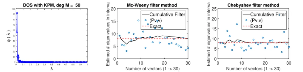
3.3.1 The McWeeny filter . . . 44
3.3.2 Chebyshev filters . . . 45
3.4 Threshold selection . . . 47
3.4.1 DOS plot analysis . . . 48
3.4.2 Algorithm . . . 50
3.5 Numerical experiments . . . 52
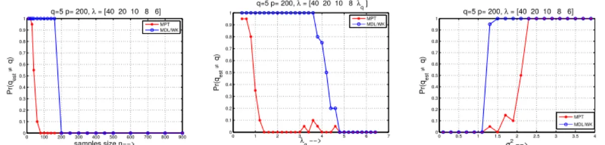
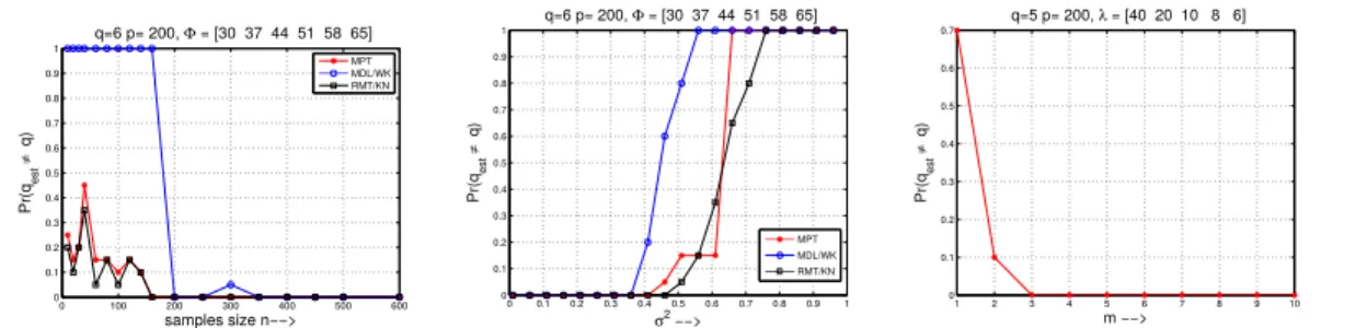
4 Dimension estimation for Krylov approximation 56 4.1 Introduction . . . 56 4.2 Problem Formulation . . . 58 4.3 Proposed Method . . . 59 4.4 Analysis . . . 61 4.4.1 Strong consistency . . . 62 4.4.2 Performance Analysis . . . 62 4.5 Numerical experiments . . . 64
4.5.1 Number of signals detection . . . 64
4.5.2 Data matrices . . . 67
5 Matrix approximations via coarsening 69 5.1 Introduction . . . 69
5.2 Applications . . . 71
5.3 Hypergraph Coarsening . . . 73
5.3.1 Multilevel SVD computations . . . 76
5.3.2 CSSP and graph sparsification . . . 76
5.4 Analysis . . . 77
5.5 Numerical Experiments . . . 81
5.5.1 Applications . . . 85
6.1 Introduction . . . 90
6.2 Incoherence via rank shrinkage . . . 92
6.3 Analysis . . . 94
6.4 Numerical Experiments . . . 98
II Applications of Coding Theory 102 7 Low rank approximation - Codes for sampling 103 7.1 Introduction . . . 103
7.2 Construction of subsampled code matrix . . . 106
7.2.1 Algorithm . . . 107
7.3 Analysis . . . 109
7.3.1 Setup . . . 109
7.3.2 Subsampled code matrices, JLT and subspace embedding . . . . 110
7.3.3 Deterministic Error bounds . . . 113
7.3.4 Error Bounds . . . 114
7.3.5 Least squares regression problem . . . 118
7.4 Choice of error correcting codes . . . 119
7.4.1 Codes with dual-distance at leastk+ 1 . . . 119
7.4.2 Choice of the code matrices . . . 120
7.5 Numerical Experiments . . . 121
8 Group testing with codes 124 8.1 Introduction . . . 124
8.2 Definitions and Notation . . . 125
8.3 Numerical Experiments . . . 126
8.4 Estimates of error probability . . . 128
9 Multilabel classification with group testing and codes 133 9.1 Introduction . . . 133
9.2 MLC via Group testing . . . 136
9.3 Constructions . . . 138
9.3.1 Random Constructions . . . 138
9.3.2 Concatenated code based constructions . . . 139
9.3.3 Expander graphs . . . 140
9.4 Error Analysis . . . 142
9.5 Numerical Experiments . . . 143
III Machine Learning for Scientific Data Applications 148 10 Union of Intersections 149 10.1 Introduction . . . 149
10.2 UoI for regression . . . 150
10.3 UoI for nononegative matrix factorization . . . 151
10.3.1 UoI-NMFcluster . . . 152
10.3.2 Numerical Experiments on Synthetic Data . . . 156
10.3.3 Experiments on Scientific Data . . . 160
10.4 UoI for CUR decomposition . . . 163
10.4.1 Experiments - Tagging gene expressions . . . 164
11 Material Informatics - Mining material data 166 11.1 Introduction . . . 166
11.2 Formation Enthalpy of metal alloys . . . 167
11.3 Machine Learning for Prediction . . . 169
11.3.1 Features Selection . . . 169
11.3.2 Machine Learning Model . . . 172
11.4 Results and Discussion . . . 173
12 Conclusion 179
References 183
List of Tables
2.1 Estimation of the sum of singular values of various matrices . . . 38
4.1 Performance of the Krylov Subspace method, Algorithm 3 withm= 10. 67 5.1 CSSP: Coarsening versus leverage score sampling. . . 83
5.2 Graph Sparsification: Coarsening versus leverage score sampling. . . 83
5.3 TaggingSNP: Coarsening, Leverage Score sampling and Greedy selection 87 5.4 Multilabel Classification using CSSP (leverage score) and coarsening. . . 88
7.1 Classes of sampling matrices with subspace embedding properties . . . . 121
7.2 Comparison of errors . . . 123
8.1 Minimum distance and average distance . . . 130
8.2 Estimates of the error probabilityfrom Theorem 10 . . . 130
8.3 Estimates of the error probabilityfrom Theorem 11 . . . 130
8.4 Estimates of the error probabilityfrom (8.5), Thm. 12 . . . 132
9.1 Dataset statistics . . . 144
9.2 MLGT v/s OvsA . . . 146
9.3 Comparisons with embedding methods. Average Test errors. . . 146
10.1 Comparison of NMF algorithms. . . 159
10.2 TaggingSNP: UoI-CUR, basic CUR and Greedy selection . . . 165
11.1 Relative errors in formation enthalpy predictions for different feature sets. 175 11.2 Predicted and actual formation enthalpies (FE) ofSc binary alloys. . . 176
List of Figures
2.1 Performance comparisons between SLQ, Chebyshev and Taylor series
ex-pansions. . . 36
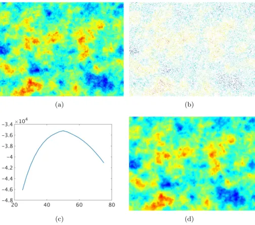
2.2 Estimation and prediction for a Gaussian random field. . . 39
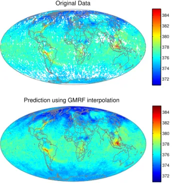
2.3 GMRF interpolation for CO2 data. . . 40
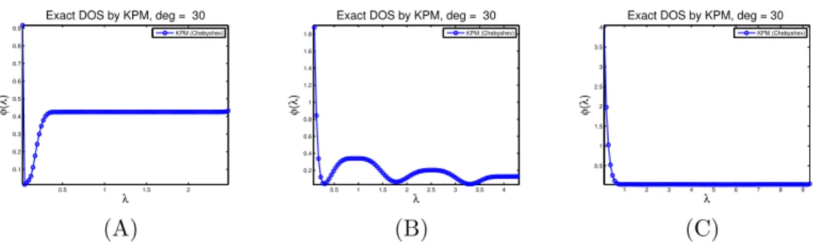
3.1 Three different scenarios for eigenvalues of PSD matrices . . . 43
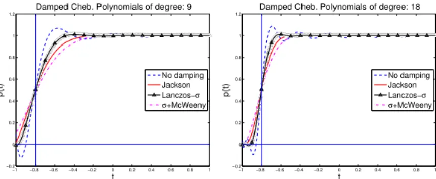
3.2 Different ways of damping Gibbs oscillations for Chebyshev approximation. 46 3.3 Exact DOS plots for three different types of matrices. . . 48
3.4 Numerical ranks estimated for the exampleukerbe1. . . 52
3.5 Rank estimation for the ORL dataset. Right: Eigenfaces. . . 53
3.6 Estimation of the number of signals for the adaptive beamforming exam-ple. . . 54
4.1 Signal detection: Comparison between proposed method MPT and MDL. 65 4.2 Signal detection: Comparison between MPT, MDL and RMT methods and Krylov method. . . 66
5.1 Results for the datasets CRANFIELD (left), MEDLINE (middle), and TIME (right). . . 82
5.2 LSI results for the MEDLINE dataset (left) and TIME dataset (right). . 85
6.1 Recovery of a random dictionary with uniform distribution. . . 99
6.2 Audio signal representations. . . 100
7.1 (Left) Randomized SVD using dual BCH code, Gaussian, SRFT and SRHT matrices as sampling matrix for input matrixKohonen. . . 122
8.1 Number of false positives with fixed-weight BCH codeword matrices and sparse random matrices, averaged over 300 trials. . . 127
8.2 Two group testing examples. . . 128
RCV1-2K for different MLGT and MLCS methods. . . 145
10.1 2D visualization of clusters of bases . . . 155
10.2 U oI-N M Fcluster for noisy Swimmer data. . . 157
10.3 U oI results for noisy MNIST two digits data. . . 158
10.4 Performance wrt. number of bootstrap resamples. . . 159
10.5 U oI-N M Fcluster results for mouse brain MSI dataset. . . 161
10.6 Rat ECoG recordings: Left ToneMap of the auditory cortex. Right -U oI-N M Fcluster bases. . . 162
10.7 U oI-CU R : Error kA−PCAkF as a function of the number of columns c. 165 11.1 Predictions of enthalpies of formation using different feature sets. . . 174
11.2 Predictions of enthalpies of formation ofSc binary alloys. . . 176
Chapter 1
Introduction
Many modern machine learning, data analysis and scientific computation applications involve operating on large dimensional matrices and datasets (sizes ranging from 104−
106). With ever increasing sizes come the necessity to develop scalable fast algorithms for handling such large dimensional data. The primary focus of this thesis is in devel-oping algorithms for high dimensional data problems with practical applications and theoretical guarantees. For this purpose, we explore ideas from different, often non-traditional, combinations of fields leading to new algorithms, new theory, and new insights in different applications. In the first part of the thesis, we explore numerical linear algebra tools to develop methods for matrix related problems. The spectrum (eigenvalue/singular value distribution) of data matrices, its functions and sums reveal various properties of the data, and are often required to be computed in numerous ap-plications. However, as the size of the data matrices increases, it becomes impractical to explicitly compute the complete spectrum of these large matrices. Hence, the devel-opment of inexpensive methods which approximately estimate these spectral quantities has become a primary focus of research in many fields.
Similarly, in many modern applications involving very large datasets (matrices), the data is typically handled via some form of matrix approximation or dimensionality re-duction. Matrix approximations and factorizations such as principal component analysis (PCA), partial singular value decompositions (SVD), CUR decompositions, graph spar-sifications, nonnegative matrix factorization (NMF), and dictionary learning are some of the popular tools used in many applications. Designing inexpensive methods for the
computation of the matrix spectral quantities and various matrix approximations for large matrices is the focus of the first part of the thesis.
Error correcting codes (ECC) have been used successfully in communication systems for several decades. In recent years, a new line of research is emerging where information theory and codes are being explored for nontraditional applications such as distributed storage systems, compressed sensing, and scientific computing. The second part of this thesis explores novel applications of ECC, particularly in solving problems related to machine learning and high dimensional data analysis. We show how unique properties of codes such as k-wise independence of codewords, orthogonality of code matrices, low coherence, error correction and others, can be exploited to develop new methods to solve various problems including low rank approximation, least squares regression, group testing, and multilabel classification.
In many scientific fields, the development of new sensing and imaging technologies has resulted in the generation of large volumes of data. These large datasets bring with them opportunities of new discoveries and insights into the fundamentals of nature. In order to realize such opportunities, the development of novel machine learning and data analysis methods is necessary. Statistical-machine learning algorithms for scientific data should satisfy the bi-criteria of returning results that are simultaneously predictive and interpretable. However, these bi-criteria are often at odds, and methods that robustly (few assumptions on the data/noise) achieve both are lacking. In the third part of this thesis, we focus on designing new learning methods that robustly extract meaningful and interpretable information from the data which arrive from different areas of science.
1.1
Thesis Overview
The underlining theme that connects the different parts of this thesis is: development of algorithms for learning from large dimensional data. The thesis comprises of three main parts.
1. Linear Algebra for Machine Learning (ML).
2. Applications of Coding Theory.
3
Part II: Appli-cations of codes Part I: Linear Algebra for ML Part III: ML for Science Thesis (3 parts)
The thesis work primarily has two key objectives. The first one is developing al-gorithms for handling large dimensional data matrices in machine learning that are computationally inexpensive and scalable. In order to develop these algorithms, we ex-plore ideas and tools from two diverse, but well-studied fields, namely, numerical linear algebra (Part I) and coding theory (Part II). The second objective is designing learning algorithms that yield interpretable results in scientific applications (Part III).
Linear Algebra for machine learning - Powerful, efficient and inexpensive (in terms of computation time and memory requirements) methods can be developed using numerical linear algebra tools to solve various problems related to large dimensional data applications. In the first part of the thesis, we explore these tools to develop methods for matrix related problems that commonly arise in machine learning and other applications. NLA for ML (5 chapters) Matrix spectral sums Matrix ap-proximations C2. Matrix function trace C3. Rank estimation C4. Krylov dimension C5. Approx. by coarsening C6. Dictio-nary learning
In most applications, the matrix related problems we encounter can be classified into two broad classes. The first class is related to the matrix spectrum, in particular, estimating spectral functions and their sums. These quantities reveal different properties of the given data matrix. The second class of matrix problems involves approximating a given matrix by smaller and/or sparser matrices in order to reduce computational and storage costs. In this thesis, we discuss the following matrix problems belonging to these two categories.
• Matrix function trace estimation: The problem of estimating the trace (sum of diagonal entries) of matrix functions such as log-determinant, Schatten norms, and spectral densities, appears often in different applications. However, explicit computation of such traces will be impractical for large matrices. This is the first problem considered in the thesis and a set of inexpensive algorithms are discussed for these trace estimations. In chapter 2, we demonstrate how a method called Stochastic Lanczos Quadrature can be employed for the fast computation of these traces. We establish theoretical results, which give multiplicative and additive error guarantees for the method. We also present few applications where the method can be useful. The results in this chapter were published in [1].
• Numerical rank estimation: In many of the data involving applications, it is often required to know the approximate rank of the data matrix at hand (approx-imate smaller dimension in which the information actually lies). In chapter 3, we consider the problem of numerical (approximate) rank estimation, and present a set of inexpensive methods, which require no matrix decomposition for the esti-mation of approximate matrix ranks. These methods were presented in [2, 3].
• Krylov dimension estimation: In many applications, it is often desired to es-timate the numerical rank of the data, and then obtain an approximation for the principal subspace associated with the numerical rank, for example in principal component analysis (PCA), subspace tracking, etc. The Krylov subspace based methods are the most popular and effective methods used for computing these ap-proximations. In chapter 4, we present a method which combines a novel criterion based rank estimator with the Krylov subspace methods to simultaneously esti-mating the numerical rank of covariance matrices and approximate the associated
5 principal subspace. The work is discussed in [4]. This work addresses two prob-lems (rank estimation and subspace approximation) simultaneously, belonging to the two classes (matrix spectrum and matrix approximation), respectively.
• Matrix approximation via coarsening: In modern applications involving very large datasets (matrices), the data is typically handled via some form of matrix approximation such as the partial SVD, column subset selection, graph sparsifica-tion and others. We propose a novel approach to compute these approximasparsifica-tions for large sparse matrices and graphs in chapter 5. The approach is based on multi-level coarsening, a popular tool used in graph partitioning and parallel computing, and is presented in [5]. This method exploits the structures available in the data and yields superior approximations.
• Dictionary learning: In signal and image processing research, the dictionary learning problem (learning a set of dictionary columns from which the matrices are derived) has received a lot of attention in recent years. Chapter 6 explores new ideas for dictionary learning using linear algebra tools. One such algorithm we develop is to learn incoherent dictionaries (distinctive dictionary columns in terms of correlation) based on rank shrinkage, published in [6]. The proposed algorithm yields improved dictionary incoherence compared to other popular methods.
Applications of coding theory - Recently, error correcting codes (ECC) have been used in nontraditional applications such as distributed storage systems, compressed sensing, and scientific computing. In the second part of this thesis, we explores novel machine learning and high dimensional data analysis applications of codes.
C8. Group testing C7. Low rank approximation C9. Multilabel classification Codes (3 chapters)
• Low rank approximation: In recent years, much attention has been devoted to randomized sampling and sketching methods for effectively approximating large matrices. In chapter 7, we demonstrate that certain error correcting codes (which are almost deterministic) mimic the randomness properties desired for sampling data matrices. Using this, we illustrate how codes can be used to obtain low rank approximations of matrices and also solve least squares regression problems. We first presented the idea in [7], and improved the theoretical results and expanded the scope of the work in [8].
• Group testing: The problem of group testing, detecting defective items from a large set of items by testing for defects in groups, has many applications in imaging, sensing, genetics, and recently in multilabel classification. We demonstrate that codewords from a popular coding scheme performs exceptionally well in group testing, and show that the proposed method outperforms traditional methods in chapter 8, first presented in [9].
• Multilabel classification: The coding theory application part of the thesis is concluded by presenting a new machine learning application for codes, that of solving large scale multilabel classification problems. Such classification problems are ubiquitous in various applications such as image, video and tweet annotation, web page categorization and others, and modern applications have a large number of classes. In chapter 9, we propose a new algorithm for multilabel classification which is based on group testing and codes. The algorithm has many promising advantages, including a simple prediction method that is very inexpensive, and it exploits the error correction capabilities of codes for the first time to correct prediction errors. We presented this multilabel classification approach in [10].
Machine learning for science - In order to explore the vast amount of complex data collected in different scientific fields, the development of novel machine learning and data analysis methods is necessary. The primary objective here is to obtain results that are interpretable from the scientific viewpoint (traditional methods fail to do so), and that are stable and robust to noise, since scientific data are typically noisy, where standard noise models fail. The last of the three parts of this thesis focuses on developing
7 such learning methods to extract meaningful information from the data which arrive from different areas of science.
ML for Science (2 chapters) C10. Union of Intersections C11. Material Informatics
• Union of Intersections: In chapter 10, we discuss a new statistical framework named Union of Intersections (UoI) for interpretable machine learning proposed in [11]. UoI is a flexible, modular, and scalable framework for statistical-machine learning problems. We demonstrate the applicability of the framework by develop-ing new algorithms for Nonnegative matrix factorization (NMF) (U oI-N M Fcluster)
and CUR decomposition (U oI-CU R) based on UoI. Modern technologies such as Electrocorticography (ECoG) have resulted in the collection of large volumes of neurophysiological data. Extracting key features from such data will provide bet-ter insight into functioning of the brain and may result in new discoveries. We employ U oI-N M Fcluster to summarize Neuroscience data with a set of few
inter-pretable bases. We presented these results in [12]. We also use the U oI-CU R
algorithm to summarize genetics data.
• Material Informatics: In recent years, the use of machine learning techniques to explore materials data is gaining popularity. In the last chapter 11 of this thesis, we examine supervised learning techniques for the study of material behavior and for material discovery. We develop a machine learning (regression) technique for the prediction of formation enthalpies of new metal alloys using easily available material data, which we presented in [13]. The goal of this work is to help by-pass time intensive calculations (some take days of computations), e.g., ab-initio calculations, used in material science.
1.2
Background
In this section, we briefly review the key background topics related to the work presented in the thesis.
1.2.1 Matrix function traces
The problem of estimating the trace of matrix functions appears frequently in appli-cations of machine learning, signal processing, scientific computing, statistics, com-putational biology and comcom-putational physics [14, 15, 16, 17]. For a symmetric ma-trix A ∈ Rn×n with an eigen-decomposition A = UΛUT, with Λ = diag(λ1, . . . , λn),
where λi, i= 1, . . . , n are the eigenvalues of A, the matrix function f(A) is defined as
f(A) = U f(Λ)UT, with f(Λ) = diag(f(λ1), . . . , f(λn)) [18]. Then the trace
estima-tion problems menestima-tioned above can be formulated as follows: given a symmetric matrix
A∈Rn×n, compute an approximation of the trace of the matrix functionf(A), i.e., tr(f(A)) =
n X
i=1
f(λi), (1.1)
where λi, i= 1, . . . , n are the eigenvalues of A, and f is the desired function. A naive
approach for estimating the trace of matrix functions is to compute this trace from the eigenvalues of the matrix, which will be expensive for large matrices. Popular trace es-timation problems include computing the log-determinant (f(t) = log(t)), the Schatten
p-norms (f(t) = tp/2), the Estrada index (f(t) = et) and the trace of matrix inverse (f(t) =t−1). In chapter 2, we present a set of inexpensive methods to approximately estimate these traces.
1.2.2 Stochastic trace estimator
Hutchinson’s unbiased estimator [19] uses only matrix-vector products to approximate the trace of a generic matrix D. The method estimates the trace tr(D) by first gen-erating random vectors vl, l = 1, . . . ,nv with equally probable entries ±1, and then
9 computing the average over the samples of vl>Dvl,
tr(D)≈ 1 nv nv X l=1 vl>Dvl. (1.2)
It is known that any random vectors vl with mean of entries equal to zero and unit
2-norm can also be used in the above computation [20]. This stochastic trace estimator can be employed in methods which compute the matrix function traces tr(f(A)) discussed above.
The convergence analysis for the stochastic trace estimator was developed in [20], and improved in [21] for sample vectors with different probability distributions. We present the convergence rate results in chapter 2. We will employ the stochastic trace estimator to compute various matrix spectrum related quantities in chapters 2 and 3.
1.2.3 Matrix factorizations and approximations
Modern applications typically handle large datasets (matrices) via some form of matrix approximation and dimensionality reduction. Here, we review some of the popular matrix factorization and approximation methods that will be considered in this thesis.
SVD and low rank approximation: Low rank approximation and principal com-ponent analysis (PCA) are the most popular dimensionality reduction methods used in numerous data related applications [22, 23]. Consider a data matrix A ∈Rm×n, with
its singular Value decomposition (SVD) A = UΣVT, where U and V are orthogonal matrices contain the left and the right singular vectors as columns, respectively, and Σ is a diagonal matrix with nonzero singular values σi, i = 1, . . . , n as diagonal entries.
For a rank k n, a rank-k approximation can be obtained as, Ak =UkΣkVkT, where
Uk andVk are matrices containing the topkleft and right singular vectors as columns,
respectively.
It is well-known that Ak = UkΣkVkT is the best rank-k approximation of A with
respect to both Frobenius and spectral norms. That is, we have from the Eckart-Young theorem [24], for ξ∈ {2, F},
min rank(X)≤k
We also know that, PCA and SVD are closely related. This is because the left singular vectors U of A are the eigenvectors of AAT and the right singular vectors V of A are the eigenvectors of ATA. Hence, in many data related applications, PCA and partial SVD are used interchangeably.
CUR decomposition: Another popular dimensionality reduction method used in many applications is column subset selection (CSSP) [25]. If even a subset of the rows are selected, then the method is called CUR decomposition [26], where C and R are matrices with the selected columns and rows, respectively, and U is the mixing matrix, such that A ≈CU R. Given a large data matrixA∈Rm×n whose columns we wish to
select, suppose Vk is the matrix associated with the top k right singular vectors of A.
Then, the leverage score of theith column of A is given by
`i=
1
kkVk(i,:)k
2 2,
the norm of the ith row of Vk. In leverage scores sampling, the columns of A are
sampled using the probability distribution pi = min{1, `i}. Most popular methods for
CSSP involve the use of this leverage scores as the probability distribution for columns selection [27, 25, 26]. However, this method is expensive since one needs to compute the topksingular vectors, which is prohibitive for large matrices. Many other closely related methods have been proposed for randomized sampling and column subset selection of matrices [28].
Graph sparsification: Sparsification of large graphs has several computational (cost and space) advantages and has hence found many applications [29, 30, 31]. Given a large graph G = (V, E) with n vertices, we wish to find a sparse approximation to this graph that preserves certain information of the original graph such as the spectral information [31, 32], structures like clusters within in the graph [29], etc. LetB ∈R(n2)×n be the vertex edge incidence matrix of the graph G, where eth row be of B for edge
e= (u, v) of the graph has a value√we in columnsu and v, wherewe is the weight of
the edge, and zero elsewhere. The corresponding Laplacian of the graph is then given by K =BTB.
11 such that if ˜Kis the Laplacian of ˜G, thenxTKx˜ is close toxTKxfor anyx∈Rn. Many
methods have been proposed for the spectral sparsification of graphs, see e.g., [31, 32, 28]. A popular approach is to perform row sampling of the matrixB using the leverage score sampling [32]. Considering the SVD of B =UΣVT, the leverage scores `i for a row bi
of B can be computed as `i = kuik22 ≤ 1 using the rows of U. This leverage score is related to the effective resistance of edge i [31]. By sampling the rows of B according to their leverage scores it is possible to obtain a matrix ˜B, such that ˜K = ˜BTB˜ and
xTKx˜ is close toxTKx for any x∈Rn.
Nonnegative matrix factorization (NMF): Since its popularization, NMF [33] has been used in many applications for obtaining interpretable decompositions of data. Given a matrix A ∈Rm+×n (R+ represents the positive orthant), where each row of A corresponds to a data point in Rn+, and a rank k, the problem of NMF is to compute the matrices W ∈Rm+×k and H∈Rk+×n, such thatA≈W H. This problem is generally posed as a non-convex optimization problem,
min
W≥0,H≥0kA−W HkF. (1.4)
Here, the rows of the matrix H form the basis of the objects (say images), and the rows of W are the encoding of the basis in the matrix A. Since both W and H are nonnegative, NMF sometimes gives more interpretable parts based decompositions, with the intuitive notion of “combining parts to form a whole” [33].
Several algorithms to solve the NMF problem have been developed to achieve various objectives, such as more interpretable results, sparser solutions, unique solutions, etc. Sparse NMF [34, 35] and convolutional NMF [36] are two popular variants of NMF. It has been claimed that NMF implicitly yields a sparse representation of the data. However, in order to obtain explicit sparse NMF solutions, the following objective function is popularly used: min W≥0,H≥0 1 2 kA−W Hk2F +λ1kWk2F +λ2 k X j=1 kH(j,:)k2p
Dictionary learning: In recent years, sparse signal approximations by means of dundant or overcomplete dictionaries have received much attention across various re-search areas, particularly in signal and image processing [37, 38]. Considering a set of signals Y = (y1, . . . , yN) with yi ∈ Rn and a redundant (overcomplete) dictionary
D ∈ Rn×k, k > n, the sparse signal approximation model assumes that the signals y i
can be represented as a sparse linear combination of the columns of D, which are also called atoms. So, we can express this model as
yi 'Dxi, i= 1, . . . , N, (1.5)
wherexi’s∈Rkare sparse vectors with a very small number of non-zero approximation
coefficients s = kxik0 n. The particularity of a dictionary learning model is that we learn the dictionary D, as well as find the sparse linear multivariate model that best describes the set of signals Y, simultaneously. The parameters of this model are determined by solving the sparse approximation problem
arg min
D∈D,X∈X
kY −DXk2F, (1.6)
wherek.kF is the Frobenius norm, andDandX are the admissible sets for the dictionary
and the approximation coefficient matrix X = (x1, . . . , xN), respectively. The set Dis
usually defined as the set of all dictionaries with unit column norm, i.e., D = {D ∈
Rn×k : kdjk2 = 1,∀j}, whereas X constrains the coefficient matrix to be sparse, i.e., the number of nonzero entries s in X is much smaller compared to the total number of entries nor X ={X ∈ Rk×N :kx
ik0 ≤ s n,∀i}. Dictionary learning starts with the set of signals Y, and aims to find both the dictionary D and the approximation coefficients matrix X. The optimization problem (1.6) is not convex and has been shown to be an NP hard problem [39]. So, the methods for solving it can only hope to achieve an approximate solution.
1.2.4 Error Correcting Codes
In communication systems, data are transmitted from a source (transmitter) to a desti-nation (receiver) through physical channels. These channels are usually noisy, causing
13 errors in the data received. In order to facilitate detection and correction of these er-rors in the receiver, error correcting codes are used [40]. A block of information (data) symbols are encoded into a binary vector1, also called a codeword. Error correcting coding methods check the correctness of the codeword received. The set of codewords corresponding to a set of data vectors (or symbols) that can possibly be transmitted is called the code. As per our definition a codeC is a subset of the binary vector space of dimension `,F`2, where`is an integer.
A code is said to be linear when adding two codewords of the code coordinate-wise using modulo-2 arithmetic results in a third codeword of the code. Usually a linear code C is represented by the tuple [`, r], where ` represents the codeword length and
r = log2|C|is the number of information bits that can be encoded by the code. There are`−r redundant bits in the codeword, which are sometimes called parity check bits, generated from messages using an appropriate rule. It is not necessary for a codeword to have the corresponding information bits as r of its coordinates, but the information must be uniquely recoverable from the codeword.
It is perhaps obvious that a linear codeC is a linear subspace of dimensionr in the vector space F`2. The basis ofC can be written as the rows of a matrix, which is known as the generator matrix of the code. The size of the generator matrixGisr×`, and for any information vector m∈Fr2, the corresponding codeword is found by the following linear map:
c=mG.
Note that all the arithmetic operations above are over the binary field F2.
To encoder bits, we must have 2r unique codewords. Then, we may form a matrix of size 2r×`by stacking up all codewords that are formed by the generator matrix of
a given linear coding scheme,
C |{z} 2r×` = M |{z} 2r×r G |{z} r×` . (1.7)
For a given tuple [`, r], different error correcting coding schemes have different generator matrices and the resulting codes have different properties. For example, for any two integers tand q, a BCH code [41] has length`= 2q−1 and dimensionr = 2q−1−tq.
1
Here, and in the rest of the text, we are considering only binary codes. In practice, codes over other alphabets are also quite common.
Any two codewords in this BCH code maintain a minimum (Hamming) distance of at least 2t+ 1 between them.
Code properties: The minimum pairwise distance between codewords is an impor-tant parameter of a code and is called just the distance of the code. As a linear code
C is a subspace of a vector space, the null space C⊥ of the code is another well de-fined subspace. This is called the dual of the code. For example, the dual of the [2q−1,2q−1−tq]-BCH code is a code with length 2q−1, dimensiontq and minimum distance at least 2q−1−(t−1)2q/2.The minimum distance of the dual code is called the dual distance of the code.
Depending on the coding schemes used, the codeword matrixC will have a variety of favorable properties, e.g., low coherence which is useful in compressed sensing [42]. Since the codewords need to be far apart, they show some properties of random vectors. We can define probability measures for codes generated from a given coding scheme. If
C ⊂ {0,1}` is an
F2-linear code whose dual C⊥ has a minimum distance abovek (dual distance > k), then the code matrix is an orthogonal array of strength k [43]. This means that, in such a code C, for any k entries of a randomly and uniformly chosen codeword c sayc0 ={ci1, ci2, . . . , cik} and for anyk bit binary stringα, we have
P r[c0 =α] = 2−k.
This is called the k-wise independence property of codes.
The codeword matrix C has 2r codewords each of length` (a 2r×`matrix), i.e., a set of 2r vectors in {0,1}`. Given a codeword c ∈ C, let us map it to a vector φ∈
R`
by setting 1−→ √−1
2r and 0 −→
1
√
2r. In this way, a binary code C gives rise to a code
matrix Φ = (φ>1, . . . , φ>2r)>. Such a mapping is called binary phase-shift keying (BPSK)
Part I
Linear Algebra for Machine
Learning
Matrix function trace estimation
2.1
Introduction
A number of problems which appear in applications of machine learning, signal process-ing, scientific computprocess-ing, statistics, computational biology and computational physics [14, 44, 45, 15, 16, 17] can all be posed as the matrix function trace estimation problem discussed in the previous chapter. The development of fast and scalable algorithms to perform this task has long been a primary focus of research in these fields. An impor-tant instance of the trace estimation problem is that of approximating log(det(A)), the log-determinant of a positive definite matrix A. Log-determinants of covariance and precision matrices play an important role in Gaussian processes and Gaussian graphical models [45]. Log-determinant computations also appear in applications such as kernel learning [46], Bayesian Learning [47], spatial statistics [48] and Markov field models [17, 49].
Another instance of the trace estimation problem in applications is that of estimat-ing Schatten p-norms, particularly the nuclear norm, since this norm is used as the convex surrogate of the matrix rank. The Schatten p-norms appear in convex opti-mization problems, e.g., in the context of matrix completion [50], in differential privacy problems [51], and in sketching and streaming models [52]. On the other hand, in uncer-tainty quantification and in lattice quantum chromodynamics [16, 53], it is necessary to estimate the trace of the inverse of covariance matrices. Estimating the Estrada index (trace of exponential function) is another illustration of the problem with applications
17 in protein indexing [44], statistical thermodynamics [54] and information theory [55].
As mentioned in the previous chapter, the naive way to compute these traces is to obtain the complete eigendecomposition of the given matrix. A popular approach to computing the log-determinant is to exploit the Cholesky decomposition [56]. Given the decomposition A = LL>, the log-determinant of A is log det(A) = 2P
ilog(Lii).
Computing the Schatten norms in a standard way would typically require the singular value decomposition (SVD) of the matrix. These methods have cubic computational complexity (in terms of the matrix dimension, i.e., O(n3) cost) in general, and are not viable for large scale applications. In this chapter, we study inexpensive methods for accurately estimating these traces for large matrices.
We study the method called “Stochastic Lanczos Quadrature” (SLQ) for approxi-mating the trace of functions of large matrices [14, 15]. The method combines three key ingredients. First, the stochastic trace estimator [19] discussed in the previous chapter is considered for approximating the trace. Next, the bilinear form that appears in the trace estimator is expressed as a Riemann-Stieltjes integral, and the Gauss quadrature rule is used to approximate this integral. Finally, the Lanczos algorithm is used to ob-tain the weights and the nodes of the quadrature rule. We establish multiplicative and additive approximation error bounds for the trace obtained by using the method. We show that the Lanczos Quadrature approximation has faster convergence rate compared to popular methods such as those based on Chebyshev or Taylor series expansions. The analysis can be extended to any matrix functions that are analytic inside a closed in-terval and are analytically continuable to an open Bernstein ellipse [57]. We consider several important trace estimation problems and their applications.
Related Work
A plethora of methods have been developed in the literature to deal with trace estimation problems. In the following, we discuss some of the works that are closely related to SLQ, particularly those that invoke the stochastic trace estimator. The stochastic trace estimator has been employed for a number of applications in the literature, for example, for estimating the diagonal of a matrix, for counting eigenvalues inside an interval [58], and for estimating the numerical rank [2, 3]. For the log-determinant computation, a few methods have been proposed, which also invoke the stochastic trace estimator.
These methods differ in the approach used to approximate the log function. Article [17] used the Chebyshev polynomial approximations for the log function. The log function was approximated using the Taylor series expansions in [59]. Article [49] provided an improved analysis for the log-determinant computations using these Taylor series expansions. Aune et. al [48] adopted the method proposed in [60] to estimate the log function. Here, the Cauchy integral formula of the log function is considered and the Trapezoidal rule is invoked to approximate the integral. This method is equivalent to using a rational approximation for the function. The method requires solving a series of linear systems and is generally expensive.
Not many fast algorithms are available in the literature to approximate the nuclear norm and Schatten-pnorms; see [52, 61] for discussions. Article [62] extends the idea of using Chebyshev expansions developed in [58, 17] to approximate the trace of various matrix functions including Schatten norms, the Estrada index and the trace of matrix inverse. Related articles on estimating the trace of matrix inverse and other matrix functions are [16, 53].
2.2
Trace estimation problems
We begin by first discussing a few trace estimation problems that arise in certain appli-cation areas.
Log-determinant: As previously mentioned, the log-determinants have numerous applications in machine learning and related fields. The logarithm of the determinant of a given positive definite matrix A ∈Rn×n, is equal to the trace of the logarithm of
the matrix, i.e.,
log det(A) =tr(log(A)) =
n X i=1
log(λi).
So, estimating the log-determinant of a matrix is equivalent to estimating the trace of the matrix function f(A) = log(A).
Suppose the positive definite matrixAhas its eigenvalues inside the interval [λmin, λmax], then the logarithm function f(t) = log(t) is analytic over this interval. When comput-ing the log-determinant of a matrix, the case λmin = 0 is obviously excluded, where
19 the function has its singularity. The Lanczos algorithm requires the input matrix to be symmetric. If A is non-symmetric, we can either consider the matrix1 A>A, since log det(ATA) = 2 log|det(A)|.
Log-likelihood: The problem of computing the likelihood function occurs in appli-cations related to Gaussian processes [45]. Maximum Likelihood Estimation (MLE) is a popular approach used for parameter estimation when high dimensional Gaussian models are used, especially in statistical machine learning. The objective in parameter estimation is to maximize the log-likelihood function with respect to a hyperparameter vector ξ: logp(z|ξ) =−1 2z > S(ξ)−1z−1 2log detS(ξ)− n 2log(2π), (2.1) where z is the data vector and S(ξ) is the covariance matrix parameterized byξ. The second term (log-determinant) in (2.1) can be computed by using the SLQ method. We observe that the first term in (2.1) resembles the quadratic form that appears in the trace estimator, and it can be also computed by using the Lanczos Quadrature method. That is, we can estimate the term z>S(ξ)−1z using m steps of the Lanczos algorithm applied toz/kzkas the starting vector, then compute the quadrature rule for the inverse functionf(t) =t−1, and rescale the result bykzk2.
Schatten p-norms: Given an input matrixX ∈Rd×n, the Schatten p-norm of X is
defined as kXkp = Pr i=1σ p i 1/p
i, where the σi’s are the singular values of X and r
its rank. The nuclear norm is the Schatten 1-norm so it is just the sum of the singular values. Estimating the nuclear norm and the Schatten p-norms of large matrices has many applications as seen earlier. Suppose we define a positive semidefinite matrix A
as1 A=X>X orA=XX>. Then, the Schattenp-norm of X is defined as
kXkp = r X i=1 λp/i 2 1/p =tr(Ap/2).
Hence, Schatten p-norms (the nuclear norm being a special case with p = 1) are the traces of matrix functions of A withf(t) =tp/2.
1
The matrix product need not be formed explicitly since the Lanczos algorithm requires only matrix vector products.
Spectral Density: Next, we consider computing the spectral density of a matrix [63], a very common problem in solid state physics. The spectral density of matrix, also known as Density of States (DOS) in physics, is a probability density distribution that measures the likelihood of finding eigenvalues of the matrix at a given point on the real line. Formally, the spectral density of a matrix is expressed as a sum of delta functions of the eigenvalues of the matrix. That is,
φ(t) = 1 n n X i=1 δ(t−λi),
where δ is the Dirac distribution or Dirac δ-function. This is not a proper function but a distribution and it is clearly not practically computable as it is defined. What is important is to compute a smoothed or approximate version of it that does not require computing eigenvalues, and several inexpensive methods have been proposed for this purpose, [64, 63]. Recently, the DOS has been used in applications such as eigenvalue problem, e.g., for spectral slicing, for counting eigenvalues in intervals (‘eigencounts’) [58], and for estimating ranks [2, 3].
Article [63] reviews a set of inexpensive methods for computing the DOS. We will further discuss the concept of DOS and its applications in Chapter 3.
Eigencount and Numerical Rank: Next, we consider counting eigenvalues located in a given interval (Eigencount) and the related problem of estimating the numerical rank of a matrix. Estimating the number of eigenvaluesη[a,b]located in a given interval [a, b] of a large sparse symmetric matrix is a key ingredient of effective eigensolvers [58], because these eigensolvers require an estimate of the dimension of the eigenspace to compute to allocate resources and tune the method under consideration. Estimating the numerical rankr =η[,λ1]is another closely related problem that occurs in machine learning and data analysis applications such as Principal Component Analysis (PCA), low rank approximations, and reduced rank regression [2, 3]. Both of these problems can be viewed from the angle of estimating the trace of a certain eigen-projector, i.e., the number of eigenvaluesη[a, b] in [a, b] satisfies:
η[a,b]=tr(P), whereP =
X λi ∈ [a, b]
21 We can interpretP as a step function ofAgiven by
P =h(A), whereh(t) =
(
1 if t ∈ [a, b]
0 otherwise . (2.2)
The problem then is to find an estimate of the trace ofh(A). A few inexpensive methods are proposed in [58, 2, 3] to approximately compute this trace. We can also compute the eigencount from the spectral density since
η[a, b]= Z b a X j δ(t−λj)dt≡ Z b a nφ(t)dt. (2.3)
The problem of numerical rank estimation is studied in chapters 3 and 4, where various methods are presented to compute the rank efficiently.
Other Applications: Other frequent matrix function trace estimation problems in-clude estimating the trace of a matrix inverse and the Estrada index.
Trace of a matrix inverse: The matrix inverse trace estimation problem amounts to computing the trace of the inverse function f(t) = t−1 of a positive definite matrix
A∈Rn×n, whose eigenvalues lie in the interval [λ
min, λmax] withλmin>0. This problem appears in uncertainty quantification and in lattice quantum chromodynamics [16, 53], where it is necessary to estimate the trace of the inverse of covariance matrices.
Estrada index: Estimation of the Estrada index of graphs is popular in computational biology. This problem accounts to estimating the trace of the exponential function, i.e.,
f(t) = exp(t). Note that, here the matrix A is the adjacency matrix of a graph, which need not be positive definite in general. However, the matrix exp(A) is always positive definite and our method and theory are applicable in this case.
2.3
Stochastic Lanczos Quadrature
The Lanczos Quadrature method was developed by Gene Golub and his collaborators in a series of articles [14, 15]. The idea of combining the stochastic trace estimator with the Lanczos Quadrature method appeared in [14] for estimating the trace of the inverse and the determinant of matrices. Given a symmetric positive definite matrixA∈Rn×n,
we wish to compute the trace of the matrix function f(A), i.e., the expression given by (1.1), where we assume that the functionf is analytic inside a closed interval containing the spectrum ofA. To estimate the trace, we invoke the stochastic trace estimator [19], which we discussed in the previous chapter. Recall that the method estimates the trace
tr(f(A)) by generating random vectors ul, l= 1, . . . ,nv, with Rademacher distribution
(vectors with ±1 entries of equal probability), forming unit vectors vl =ul/kulk2, and then computing the average over the samples v>l f(A)vl:
tr(f(A))≈ n nv nv X l=1 vl>f(A)vl. (2.4)
Hence, for computing the trace we only need to estimate the scalars of the formv>f(A)v, and the explicit computation of f(A) is never needed.
The scalar (quadratic form) quantitiesv>f(A)vare computed by transforming them to a Riemann-Stieltjes integral, and then employing the Gauss quadrature rule to ap-proximate this integral. Consider the eigen-decomposition of A as A =QΛQ>. Then, we can write the scalar product as,
v>f(A)v=v>Qf(Λ)Q>v=
n X
i=1
f(λi)µ2i, (2.5)
where µi are the components of the vector Q>v. The above sum can be considered as
a Riemann-Stieltjes integral given by,
I =v>f(A)v= n X i=1 f(λi)µ2i = Z b a f(t)dµ(t), (2.6)
where the measure µ(t) is a piecewise constant function defined as
µ(t) = 0, ift < a=λ1, Pi−1 j=1µ2j, ifλi−1≤t < λi, i= 2, . . . , n, Pn j=1µ2j, ifb=λn≤t, (2.7)
23 estimated using the Gauss quadrature rule [15]
Z b a f(t)dµ(t)≈ m X k=0 ωkf(θk), (2.8)
where{ωk}are the weights and{θk}are the nodes of the (m+1)-point Gauss quadrature,
which are unknowns and need to be determined.
An elegant way to compute the nodes and the weights of the quadrature rule is to use the Lanczos algorithm [15]. For a given real symmetric matrixA∈Rn×n and a starting
vectorw0 of unit 2-norm, the Lanczos algorithm generates an orthonormal basis Wm+1 for the Krylov subspace Span{w0, Aw0, . . . , Amw0} such that Wm>+1AWm+1 = Tm+1, where Tm+1 is an (m+ 1) ×(m+ 1) tridiagonal matrix. For details see [56]. The columns wk of Wm+1 are related as
wk =pk−1(A)w0, k= 1, . . . , m,
where pk are the Lanczos polynomials. The vectors wk are orthonormal, and we can
show that the Lanczos polynomials are orthogonal with respect to the measure µ(t) in (2.7); see Theorem 4.2 in [15]. Therefore, the nodes and the weights of the quadrature rule in (2.8) can be computed as the eigenvalues and the squares of the first entries of the eigenvectors of Tm+1. Then, we can approximate the quadratic form (2.5) as,
v>f(A)v≈ m X k=0 τk2f(θk) with τk2= h e>1yk i2 , (2.9)
where (θk, yk), k = 0,1, ..., m are eigenpairs of Tm+1 by using v as the starting vector
w0. Thus, the trace of matrix function f(A) can be computed as,
tr(f(A))≈ n nv nv X l=1 m X k=0 (τk(l))2f(θ(kl)) ! , (2.10)
where (θk(l), τk(l)), k = 0,1, ..., mare eigenvalues and the first entries of the eigenvectors of the tridiagonal matrix Tm(l)+1 corresponding to the starting vectors vl, l = 1, . . . ,nv.
purpose of computing the trace via (1.1). The Stochastic Lanczos Quadrature algorithm corresponding to this procedure is summarized in Algorithm 1.
Algorithm 1 Trace of a matrix function by SLQ using the Lanczos algorithm
Input: SPD matrixA∈Rn×n, functionf, degree m and nv.
Output: Approximate trace Γ of f(A).
forl= 1 to nv do
1. Generate a Rademacher random vectorul and form unit vectorvl=ul/kulk2
2. T = Lanczos(A, vl, m+ 1); that is, applym+ 1 steps of Lanczos toAwithvl as
the starting vector.
3. [Y,Θ] =eig(T) and computeτk = [e>1yk] for k= 0, . . . , m 4. Γ←Γ +Pm k=0τk2f(θk). end for Output Γ = nn vΓ.
2.4
Analysis
One of the main contributions of this chapter is the derivation of multiplicative error bounds for approximating the trace of a matrix function using SLQ. Additive error bounds are also established for the log-determinant approximation of a positive definite matrix and the log-likelihood function estimation. The nuclear norm and Schatten-p
norms estimation of a general matrix is discussed in the latter part of the section. First, we give the following definition: A Bernstein ellipse Eρ is an ellipse on the complex
plane with focii at −1,1 and major semi-axis (ρ+ρ−1)/2, with ρ > 1 [57]. It can be viewed as a mapping of the circle C(0, ρ) (center at zero and radius ρ) using the Joukowsky transform (z+z−1)/2. Hence we can have two values ofρ that are inverses of each other, which give the same ellipse. Following is our main result:
Theorem 1 Consider a symmetric positive definite matrixA∈Rn×n with eigenvalues
in [λmin, λmax] and condition number κ = λmax/λmin. Let f be a function analytic in [λmin, λmax] and be either positive or negative (i.e., does not cross zero) inside this interval. Denote by mf the absolute minimum value off in the interval. Assume that
25 with foci λmin, λmax and sum of the two semi-axes ρ, such that |f(z)| ≤ Mρ for all
z∈Eρ. Let , η be constants in (0,1). Then for SLQ parameters satisfying:
• m≥ 1 2log 4M ρ(λmax−λmin) mρ(ρ2−1)
/log(ρ) number of Lanczos steps, and
• nv ≥(24/2) log(2/η) number of starting Rademacher vectors,
the output Γ of the Stochastic Lanczos Quadrature method is such that:
Pr
|tr(f(A))−Γ| ≤|tr(f(A))|
≥1−η. (2.11)
In particular for ρ= (√κ+ 1)/(√κ−1), for which the function of interest is analytic insideEρ, we havem≥(
√
κ/4) log(K/), withK= (λmax−λmin)(
√
κ−1)2Mρ/(
√
κmf).
To prove the theorem, we first derive error bounds for the Lanczos Quadrature approximation (which gives the convergence rate), using the facts that an (m+ 1)-point Gauss Quadrature rule is exact for any 2m+ 1 degree polynomial and that the function is analytic inside an interval and is analytically continuable in a Bernstein ellipse. We then combine this bound with the error bounds for the stochastic trace estimator to obtain the above result.
Convergence rate for the Lanczos Quadrature
In order to prove Theorem 1, we first establish the convergence rate for the Lanc-zos Quadrature approximation of the quadratic form. Recall that the quadratic form
v>f(A)v can be written as a Riemann Stieltjes integral I, as given in (2.6). Let Im
denote the (m+ 1)-point Gauss Quadrature rule that approximates the integralI, given by Im = m X k=0 ωkf(θk),
where {ωk} are the weights and {θk} are the nodes, computed by using m+ 1 steps of
the Lanczos algorithm. The well known error analysis for the Gauss Quadrature rule is given by [15], |I−Im|= f(2m+2)(ζ) (2m+ 2)! Z b a m Y k=0 (t−θk) 2 dµ(t), (2.12)
for some a < ζ < b. However, this analysis might not be useful for our purpose, since the higher derivatives of both the logarithm and the square root function become excessively large in the interval of interest. Hence, in this work, we establish improved error analysis for the Lanczos Quadrature approximations, using some classical results developed in the literature, with the fact that functions of interest are analytic over a certain interval. We begin with the following result.
Theorem 2 Let a function g be analytic in [−1,1]and analytically continuable in the open Bernstein ellipseEρwith foci±1 and sum of major and minor axis equal toρ >1,
where it satisfies|g(z)| ≤Mρ. Then the(m+1)-step Lanczos Quadrature approximation
satisfies
|I −Im| ≤
4Mρ
(ρ2−1)ρ2m. (2.13)
Proof. We follow a similar argument developed in [65] that estimates the error of Gaussian quadratures for a Riemann integral. The result and the proof strategy are usually covered in standard textbooks, e.g., [57, Thm. 19.3]. In our case, the integral is a Riemann-Stieltjes integral with respect to a specific measure given in (2.7). As a result, the bound admits the same rate but with a different constant.
For the given functiongthat is analytic over the interval [−1,1], consider the 2m+ 1 degree Chebyshev polynomial approximation of g(t), i.e.,
P2m =
2m+1
X j=0
ajTj(t)≈g(t).
We know that the (m+ 1)-point Gauss Quadrature rule is exact for any polynomial of degree upto 2m+ 1, see [15, Thm. 6.3] or [57, Thm. 19.1]. This can also be deduced from the error term in (2.12). Hence, the error in integratingg is the same as the error in integrating g−P2m. Thus, we have
|I−Im| = |I(g−P2m)−Im(g−P2m)| ≤ |I(g−P2m)|+|Im(g−P2m)| = I ∞ X j=2m+2 ajTj(t) + Im ∞ X j=2m+2 ajTj(t) ≤ ∞ X j=2m+2 |aj| |I(Tj)|+|Im(Tj)|
27 Next, we obtain bounds for the three terms inside the summation above.
If the function g is analytic in [−1,1] and analytically continuable in the Bernstein ellipse Eρ, then for the Chebyshev coefficients we have from Theorem 8.1 in [57] and
eq. (14) in [65],
|aj| ≤
2Mρ
ρj .
Next, for the Quadrature rule Im(Tj), we have
Im(Tj) = m X k=0 τk2Tj(θk)≤ m X k=0 |τk2||Tj(θk)| ≤1.
The last inequality results from the fact that, forf(t) = 1, the quadrature rule is exact, and the thus integral is equal to 1 (v>l f(A)vl = v>l vl = 1). Therefore, the weights τk2
must sum to 1. The maximum value of Tj inside the interval is 1. Finally, in order to
bound the Riemann-Stieltjes integral I(Tj), we use the following:
I(Tj) =v>Tj(A)v≤λmax(Tj(A)) = 1,
by the min-max theorem andkvk= 1. Therefore,
|I−Im| ≤ ∞ X j=2m+2 2Mρ ρj [1 + 1].
Since the Gauss quadrature rule is a symmetric rule [65], the error in integration of
Tj(t) for any oddj will be equal to zero. Thus, we get the result in the theorem
|I −Im| ≤
4Mρ
(ρ2−1)ρ2m.
Remark 1 The convergence rate for the Chebyshev polynomial approximation of an analytic function is O(1/ρm); see Theorem 8.2 in [57]. Hence, the Lanczos Quadrature
approximation is twice as fast as the Chebyshev approximation. Moreover, it is known that the Gauss quadrature has the maximal polynomial order of accuracy [57].
Theorem 2 holds for functions that are analytic over [−1,1]. The functions consid-ered in this paper such as logarithm, exponential and square root functions are analytic over [λmin, λmax] forλmin>0. Hence, we need to use the following transform to get the right interval.
Iff(x) is analytic on [λmin, λmax], then
g(t) =f λmax−λmin 2 t+ λmax+λmin 2
is analytic on [−1,1]. If we denote the error in the Quadrature rule for approximating the integral of function f asE(f), then we have
E(f) = λmax−λmin 2 E(g).
The function g will have its singularity at t0 = α = −κκ+1−1. Hence, we choose the ellipse Eρ with the semimajor axis length of |α| where g is analytic inside. Then, the
convergence rate ρwill be
ρ=α±pα2−1 =
√
κ+ 1
√
κ−1 >1.
The sign is chosen such thatρ >1. From theorem 2, the errorE(g)≤4Mρ/[(ρ2−1)ρ2m],
where |g(z)|< Mρ insideEρ. Hence, the error E(f) will be
E(f) = λmax−λmin 2 4Mρ (ρ2−1)ρ2m = (λmax−λmin)( √ κ−1)2Mρ 2√κρ2m ,
with ρ defined as above. Thus, for a function f that is analytic on [λmin, λmax] and
Cρ= 2Mρ(λmax−λmin)/(ρ2−1) = (λmax−λmin)(
√ κ−1)2Mρ/(2 √ κ), we have v>f(A)v− m X k=0 τk2f(θk) ≤ Cρ ρ2m. (2.14)
Approximation error of the trace estimator
The quadratic form v>f(A)v for which we derived the error bounds in the previous section comes from the Hutchinson trace estimator. Let us denote this estimator as
29
trnv(A) =
n
nv
Pnv
l=1vl>Avl. The convergence analysis for the stochastic trace estimator
was developed in [20], and improved in [21] for sample vectors with different probability distributions. We state the following theorem which is proved in [21].
Theorem 3 Let A be an n ×n symmetric positive semidefinite matrix and vl, l =
1, . . . ,nv be random starting vectors sampled from the Rademacher distribution and scaled to a unit 2-norm. Then, with nv≥(6/2) log(2/η), we have
Pr [|trnv(A)−tr(A)| ≤|tr(A)|]≥1−η.
The above theorem can be used to bound the trace of any matrix functionf(A), if the function is either positive or negative inside the spectrum interval. Therefore, the theorem holds for the square root function, its powers, and the exponential. However, for the logarithm function, different scenarios occur depending on the spectrum, which will be discussed later. Let Γ be the output of the Stochastic Lanczos Quadrature method to estimate the trace of such functions, given by
Γ = n nv nv X l=1 m X k=0 (τk(l))2f(θ(kl)) ! . (2.15)
We need the following lemma.
Lemma 1 Let A ∈ Rn×n be a symmetric positive definite matrix with eigenvalues in
[λmin, λmax]and condition numberκ=λmax/λmin, and f be an analytic function in this interval with |f(z)| ≤Mρ, for all z inside a Bernstein ellipse Eρ that encompasses the
interval. Then, the following inequality holds:
|trnv(f(A))−Γ| ≤ nCρ
ρ2m,
where ρ= (√κ+1)/(√κ−1)andCρ= 2Mρ(λmax−λmin)/(ρ2−1) = (λmax−λmin)(
√
κ−
1)2Mρ/(2
√
Proof. The lemma follows from the equation (2.14). We have |trnv(f(A))−Γ| = n nv nv X l=1 vl>f(A)vl− nv X l=1 Im(l) ≤ n nv nv X l=1 |vl>f(A)vl−Im(l)| ≤ n nv nv X l=1 Cρ ρ2m = nCρ ρ2m.
Now, we are ready to prove Theorem 1. Based on the condition ofm,
logK ≤ 4m √ κ ≤2mlog √ κ+ 1 √ κ−1 . Therefore, K ≤ρ 2m and hence Cρ ρ2m ≤ 2fmin(λ),
wherefmin(λ)≡mf is the absolute minimum of the function in the interval [λmin, λmax]. This gives us the lower bound on the degree m in the Theorem. Then, from Lemma 1 we have |trnv(f(A))−Γ| ≤ n 2 fmin(λ)≤ 2|tr(f(A))|. (2.16) From Theorem 3, we have
Pr h |tr(f(A))−trnv(f(A))| ≤ 2|tr(f(A))| i ≥1−η. (2.17)
Combining the above two inequalities (2.16) and (2.17) leads to the result in Theorem 1: 1−η ≤ Pr h |tr(f(A))−trnv(f(A))| ≤ 2|tr(f(A))| i ≤ Pr h |tr(f(A))−trnv(f(A))|+|trnv(f(A))−Γ| ≤ 2|tr(f(A))|+ 2|tr(f(A))| i ≤ Pr [|tr(f(A))−Γ| ≤|tr(f(A))|].