Crater Detection via Genetic Search Methods to Reduce Image Features

University of Massachusetts Boston

ScholarWorks at UMass Boston

Graduate Masters Theses Doctoral Dissertations and Masters Theses

12-31-2013

Crater Detection via Genetic Search Methods to

Reduce Image Features

Joseph Paul Cohen

University of Massachusetts Boston

Follow this and additional works at:http://scholarworks.umb.edu/masters_theses

Part of theComputer Sciences Commons, and theGeographic Information Sciences Commons Recommended Citation

Cohen, Joseph Paul, "Crater Detection via Genetic Search Methods to Reduce Image Features" (2013).Graduate Masters Theses.Paper 207.

CRATER DETECTION VIA GENETIC SEARCH METHODS TO REDUCE IMAGE FEATURES

A Thesis Presented by

JOSEPH PAUL COHEN

Submitted to the Office of Graduate Studies, University of Massachusetts Boston,

in partial fulfillment of the requirements for the degree of

Master of Science

December 2013

© 2013 by Joseph Paul Cohen All rights reserved

CRATER DETECTION VIA GENETIC SEARCH METHODS TO REDUCE IMAGE FEATURES

A Thesis Presented by

JOSEPH PAUL COHEN

Approved as to style and content by:

Wei Ding, Assistant Professor Chairperson of Committee

Dan A. Simovici, Professor Member

Nurit Haspel, Assistant Professor Member

Dan A. Simovici, Program Director Computer Science Program

Peter Fejer, Chairperson Computer Science Department

ABSTRACT

CRATER DETECTION VIA GENETIC SEARCH METHODS TO REDUCE IMAGE FEATURES

December 2013

Joseph Paul Cohen,

A.S., Massachusetts Bay Community College B.S., University of Massachusetts Boston

Directed by Assistant Professor Wei Ding

Recent approaches to crater detection have been inspired by face detection’s use of gray-scale texture features. Using gray-scale texture features for supervised machine learning crater detection algorithms provides better classification of craters in planetary images than previous methods. When using Haar features it is typical to generate thousands of numerical values from each candidate crater image. This magnitude of image features to extract and consider can spell disaster when the application is an entire planetary surface. One solution is to reduce the number of features extracted and

considered in order to increase accuracy as well as speed. Feature subset selection

provides the operational classifiers with a concise and denoised set of features by reducing irrelevant and redundant features. Feature subset selection is known to be NP-hard. To provide an efficient suboptimal solution, four genetic algorithms are proposed to use greedy selection, weighted random selection, and simulated annealing to distinguish discriminate features from indiscriminate features. Inspired by analysis regarding the

relationship between subset size and accuracy, a squeezing algorithm is presented to shrink the genetic algorithm’s chromosome cardinality during the genetic iterations. A significant increase in the classification performance of a Bayesian classifier in crater detection using image texture features is observed.

TABLE OF CONTENTS

LIST OF TABLES . . . vii

LIST OF FIGURES . . . viii

CHAPTER Page 1. INTRODUCTION . . . 1

2. BACKGROUND AND METHOD . . . 5

Related Work . . . 6

Genetically Enhanced Feature Selection . . . 9

Algorithms . . . 14

3. EXPERIMENTS . . . 24

4. CONCLUSION . . . 36

LIST OF TABLES

Table Page

LIST OF FIGURES

Figure Page

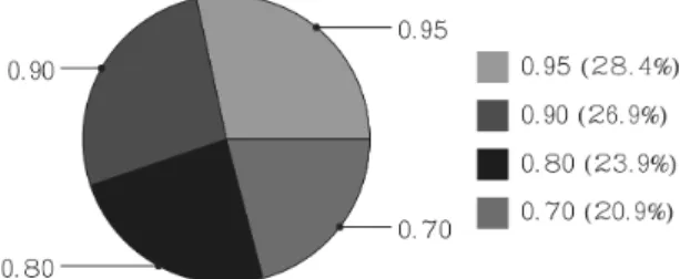
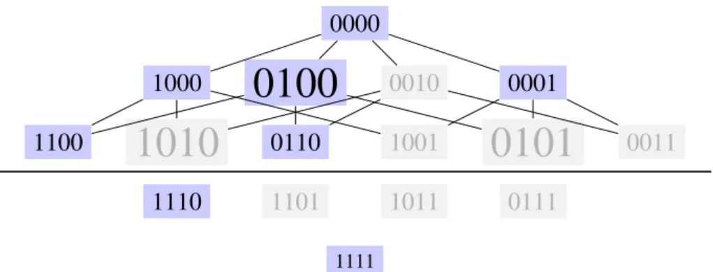
1. Shown here is diagram based on one used by Kohavi to represent the search space for 4 features [KJ97]. Each vertex is a possible subset of features and it’s size represents the result of it’s evalua-tion funcevalua-tion in relaevalua-tion to other verticies. Vertices that have been visited by the algorithm are colored blue and unvisited in gray. . . . 10 2. Sample F1 values of subsets given proportional value in the pie

chart based on their computednorm values. The edge of the pie chart is taken up based on the F1 score of the subset. . . 17 3. This brick chart details the GetWeightedSubset function in

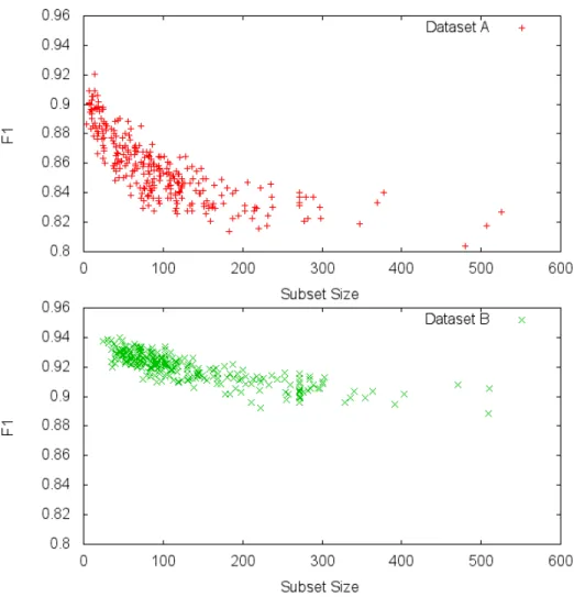
Algo-rithm 2.3.2. It shows the subsets depicted in Figure 2 but as rect-angles side by side. Each block contains it’s fitness score and also it’s normalized fitness value. . . 17 4. Subset size distributions and their F1 score on the datasets. These

are the resulting subsets from over 1200 runs of the algorithm. It is clear that the smaller the subset size the better the F1 is. . . 20 5. The SCCS algorithm restricts the search space by eliminating higher

cardinality vertices from selection. This upper bound is constructed with the mean of the highest performing vertices. Each vertex is a possible subset of features and it’s size represents the result of it’s evaluation function in relation to other vertices. . . 21 6. Datasets A (left) and B (right) are composed of 2 square sections

of the HRSC nadir panchromatic image h0905 0000 from [HRS]. The ground truth is overlaid on the image in white. The tile names from our public datasets are as follows. Dataset A is composed of 2 24 and 2 25 while Dataset B is composed of 3 24 and 3 25 . . . 25 7. Left: Crater detection pipeline, Right: Haar Masks used to extract

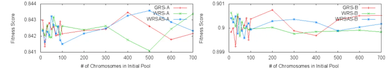
8. This figure shows the impact of the size of the initial pool of fea-tures subsets on the resulting F1 value of the final subset. The average of over 5000 runs of the algorithm are presented. For this experiment each run consisted of 1000 iterations, a population of 10 subsets, and a mutation rate of 1% Top: Dataset A, Bottom: Dataset B . . . 27 9. Average Percentage of Mutation verses fitness and resulting subset

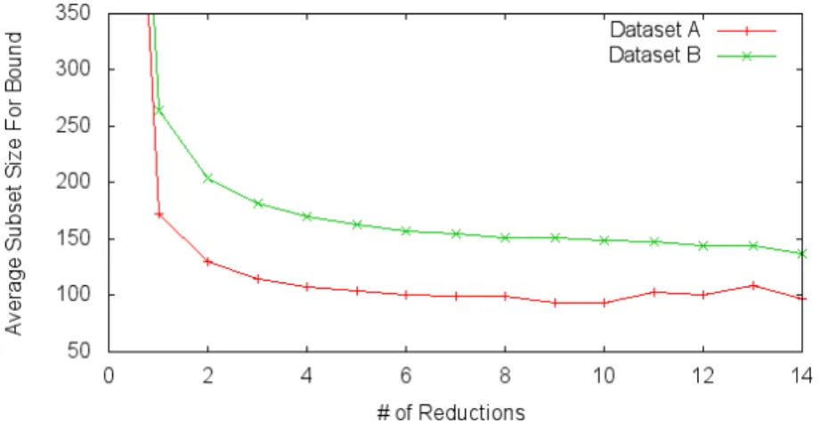
size. Left: fitness, Right: resulting subset size. The average of over 5000 runs of the algorithm are presented. The parameters for these experiments were Iterations=1000, Population=10, and Initial Pool=10. Top: Dataset A, Bottom: Dataset B . . . 29 10. The average bound size after x reductions on the datasets. The

starting bound, not shown, is the total numbers of features, 1089. . 30 11. Mutation rate effect on subset fitness using the SCCS method

con-figured with 5 reduction steps of 1000 iterations each, and a popu-lation and initial pool of 10.Top: Dataset A, Bottom: Dataset B . . 31 12. Comparison between the genetic feature selection process without

correcting the maximum size of the chromosome and a process that corrects the maximum size to be the mean size of the top per-forming chromosomes. . . 32 13. Overall results of all methods presented during 10-fold cross

val-idation. Left: Best average F1 scores, Right:Best average subset sizes, Top: Dataset A, Bottom: Dataset B . . . 33 14. Here the number of input features to the SCCS method is varied

from 50 to 1000 and binned into groups of 100. The average time required to perform the feature selection and train the classifier is shown over 500 experiments. SCCS is configured with 15 re-ductions with 1000 iterations each. The bottom half of dataset B (containing 727 instances) is used as a training set. . . 34

15. Here SCCS is used with 15 reductions of 1000 iterations each. A classifier for each half of the dataset is built using the other half (top/bottom). Correct detections are shown as a white circle. False detections, both positive and negative are shown as a red square. We achieve 0.844 accuracy on Dataset A and 0.888 on Dataset B. Classification of each instance took 0.5ms. . . 35

CHAPTER 1

INTRODUCTION

Craters are among the most studied geomorphic features in the Solar System because they yield important information about the past and present geological processes and provide the only tool for measuring relative ages of observed geologic formations. The work presented in this paper utilizes machine automation for crater detection.

A major challenge for planetary scientists is the magnitude of data available from missions to other planets such as Mars. With every mission to mars capturing higher and higher resolution imagery, the data to process will only grow. The High Resolution Stereo Camera [HRS] camera captures 12.5 meters per pixel and it’s successor High Resolution Imaging Science Experiment [HiR] captures 50 cm per pixel. Automatic methods to process this data are not trivial.

A previous study by [Tan86] concluded that the distribution of craters is exponential in relation to their size on Mars. This work aims to detect sub-kilometer craters and so must be able to deal with an exponential growth in complexity to analyse and draw significant new results on existing regions. This could result in billions of craters being identified on the surface of Mars during future planetary research.

If a scalable high-accuracy solution can be found it will enable many studies on large regions of planetary bodies including determining the geologically active regions of a

planet, relatively dating sections of a planet, and determining both landing and exploration sites for interplanetary probes/machines.

Classifiers primarily operate on numerical instance vectors. The challenge is to create an effective mapping between crater detection and machine learning classification

problems. The classifier is trained with instance vectors that are labeled and can then label instance vectors themselves. A trivial mapping into a standard machine learning problem would be to use sliding windows to generate candidates and have each pixel be an feature in the candidate. This is infeasible due to the large size and number of planetary images. This problem space must be reduced to something solvable in a reasonable amount of time.

Using techniques described by [BDS10] we can generate crater candidates using the highlight and shadow regions as well as the circular shape to narrow down the crater search space of a large image. This method of generating candidates is usable because it retains high recall. However it must be complemented with machine learning to increase the accuracy to a usable level. Haar feature masks were a breakthrough tool in face detection by [VJ04] because of their high accuracy and ability to achieve the speed necessary for real time face detection. These candidates can be processed using Haar feature masks to generate instance vectors for a classifier.

This previous research has reduced crater detection to machine learning. There are still problems that inhibit this pipelines ability to achieve high accuracy. One impediment is the number of Haar feature masks that must be generated for high accuracy. Crater detection is a harder task than face detection. The distinction between faces and other objects is more apparent than cratered ground and noncratered ground. Craters have rims that are circular but when aged they appear as piles of rubble. While detecting craters, both fresh and aged craters must be detected with high accuracy. Rubble piles can be

mistaken for rims of aged craters which makes it very hard to draw a solid line between crater and noncrater. The blur of this line is noise to the classifier that will both increase runtime with irrelevant crater features as well as reduce performance.

There are many crater features available in visible imagery from both simple and complex craters [Pik80]. For instance ejecta blankets surrounding craters provide a consistent frame for cropped crater imagery. Center uplifts and central peeks provide distinctive discrimination between unimpacked and overimpacked soil. The algorithm is designed to detect multi-anglular age-invariant impact craters with one single generic supervised algorithm that is robust enough for planetary scientists to automate their work.

The state of the art method of crater detection involves utilizing texture and contrast features of crater image candidates described by [DSM11] and [BDS11]. This is achieved by extracting many numerical features from an image, each representing a particular texture or contrast, constructing a representative instance vector, and then applying machine learning to decide if potential crater images are in fact craters. Haar features, a gray-scale image texture features, are especially useful because of their ability to be calculated in near constant time using a data structure called integral images described by [VJ04].

The challenge in using Haar features is that the number of Haar features can easily be tens of thousands. Many Haar features are redundant or even irrelevant. [DSM11] used AdaBoost to select crater image features and boost performance to between 79-90%. This paper aims to validate and improve those results.

Our work of machine learning applied to discriminative image features makes certain assumptions that are not considered when using AdaBoost. Each feature generated from the candidate crater images can be broken down into discriminate features and

classification. Indiscriminate features provide no information to the classifier or

misguiding information. Instead of weighting these features some negligible amount and continuing to extract them; they are simply removed.

To solve this new problem we want to find a subset of crater features that consists of only relevant features. By removing redundant and irrelevant features we both speed up classification and improve accuracy. There are two methods of feature selection we can use. Filter methods use domain knowledge to remove crater features without

consideration of the class label. On the other hand, wrapper methods explicitly use the class label to validate the quality of a subset of features. Wrapper methods provide higher accuracy when finding subsets because they take the global classification rates into account. The downside to wrapper methods is that they have aO(2n)price tag to find the optimal solution. This computational cost can be mitigated using a variety of methods.

In this paper we present feature subset selection methods to find a high performing subset of features for a given classifier. Feature subset selection is known to be NP-hard. Exhaustive search is the only way to find the optimal subset of a set of features. To find, for certain, the optimal solution all permutations must be considered. The search space is 2f where f is the number of features. For an example with only 58 features it would take 91 million years to compute all classifiers if a classifier took 0.10 seconds to create and evaluate.

CHAPTER 2

BACKGROUND AND METHOD

By the design of our feature extraction process, thousands of contrast image features can be extracted and many will be redundant or even irrelevant. A subset of these features can achieve higher accuracy when selected properly [CLD11, LDC11]. Our feature selection methods apply beyond the scope of crater detection and can apply to any wrapper based feature selection problem.

Once Haar features have been extracted from the candidate image we choose only those that are relevant and discriminative to our crater objective. This will not only increase the speed of the classifier but will increase the accuracy as well. Removing redundant and irrelevant features saves time during the feature extraction process because they don’t have to be written to disk or sent over a network. It also saves time during the classification process because a classifier does not have to consider these features during it’s classification phase.

In this paper we extend the three genetic algorithms presented in [CLD11] with new figures, explanations, and analysis. We also present a new modification to increase classifier performance without incurring a higher cost. An overview of the content of this publication follows:

• Four genetic algorithms are presented in total, each builds on the previous to increase the classification rate for our crater detection datasets.

• Three genetic parent selection algorithms are presented using the approaches of highest fitness selection, weighted random selection, and simulated annealing to select discriminate features that a classifier will use to classify images

• This paper shrinking cardinality chromosome genetic algorithm is presented to simultaneously reduce the resulting subset size while increasing the resulting fitness score.

• We provide an in depth analysis of a real world large dataset that is currently a challenge in the field.

2.1 Related Work

Crater detection is a well studied field of research along with many image object detection objectives. There have been many methods used to automatically detect craters. A few have incorporated genetic algorithms in different ways. The method proposed by [HIK02] builds a SOM using Hough transforms to extract geometric features, then performs best parameter selection to reduce duplicate detections using a genetic algorithm based on the center location and radius of the detected crater. A method by [DA10] applies genetic algorithms to fit an ellipse to the rim of a crater using detected edges. A method by [BPA03] named GENIE uses genetic algorithms to build candidate image-processing algorithms based on a predefined set of image filters.

[Mic03] first explored the concept of global automatic coverage in adjusting the catalogued coordinates of the approximately 20,000 craters on Mars exceeding 10kmin diameter. The goal here was to use an automated method to correct an existing dataset. This method employed Hough Transforms and focused on the circularity of the craters. [SU08] performed a global martian survey resulting in 75,919 craters ranging in size from

1.36kmto 347kmby identifying round depressions in the surface and then applying machine learning for higher accuracy. [SLM12] applied fuzzy edge detection and presents global coverage. Salamuniccar has many works relating to global coverage including [SL10, SL08] on Mars and [SLP11] on Phobos. One major connection between the above methods is that they all use DEM based datasets to achieve global coverage.

Visual imagery has many advantages over DEM datasets. Visual imagery is usually of higher resolution than DEM datasets. Visual imagery is also available in areas where DEM datasets are not. Our dataset contains 4 (1700 x 1700 pixel) tiles which represents 0.27% of the THEMIS Day IR Global Mosaic which is 92160 x 46080 pixels at 256 ppd.

[BSP07] utilized visual images and template matching to identify craters. This has been followed by many more works using visual imagery that form the basis for this work such as [BDS10], [LDC11], and [DSM11] which are discussed in detail later.

At the core of all crater detection methods there is some form of a classifier either implicit or explicit. This paper uses standard classification methods to determine the probability that an image is in fact a crater as inspired by [DSM11] and [BDS10]. The most similar indirect research has been [CJM03]. Y. Cheng used the concept of a

confidence evaluation to detect craters and [KMV05] used a fitness check to determine if the candidate was a crater or not.

This work utilizes Haar features to perform candidate image classification. Haar features were used by [DSM11], [BDS10], and [LDC11] and are the state of the art in crater detection because of their adaptive and discriminative ability. They are used in this work as crater image features. Haar features were first proposed by [POP98], then applied to face detection by [VJ04], and then applied to crater detection by [DSM11]. Haar features are attractive because the use of integral images can speed up the calculation of

Haar features to O(1) on average. [VJ04] showcased by the feasibility of using these features in domains which demanded performance.

Feature subset selection can be categorized into embedded approaches, filter approaches, and wrapper approaches. Embedded approaches naturally select features while a data mining algorithm is performed. For example, decision tree classifiers [BHV95, CS96]. Filter methods evaluate subset of features independent of learning algorithms [Hal99, KS96]. Filter methods were used as early as [AD91]. Filter methods combine feature selection and classifier evaluation. features are added or removed based on statistical measures instead of an induction algorithm. Wrapper methods by

[JKP94, DK82, CF94] use a specific data mining algorithm to evaluate a feature subset to guide their decisions to include or exclude a feature.

In this paper, we use a wrapper method to select features for a classifier. This is a very popular method in the field of machine learning but has only been applied to crater

detection in this line of research. A wrapper method was coined by [JKP94], but the technique was used originally by [DK82]. A collection of subsets combined with a wrapped classifier creates a space that has been explored before with various techniques. Greedy search was attempted by [CF94] and discovered that adding and removing features yielded better results. [KJ97] used forward and backward best-first search to search for subsets, but this approach is not suited for situations where there are significantly more irrelevant variables than relevant ones [SU04]. Genetic Algorithms have also been applied to this problem by [VD95], [CS96], and [ILE00].

This work extends our previous work in [CLD11] by including more detailed analysis of the datasets and method as well as a shrinking cardinality chromosome method. The shrinking cardinality chromosome method offers a significant increase in performance in conjunction with the genetic algorithm.

2.2 Genetically Enhanced Feature Selection

This section presents four genetic algorithms used for feature subset selection. Each algorithm builds upon the one before it in an attempt to achieve better results. The first algorithm is explained in detail and then only modifications are explained for the next three algorithms. First the main concepts of genetic algorithms, genetic representation, and fitness are discussed. For each algorithm there is an initial plan, explanation of steps, and a complexity analysis.

What we aim to maximize with these algorithms is a fitness function detailed in section 2.2.2. We use the F1 metric to evaluate classifiers built with the subsets that we generate. This allows a multiobjective approach focusing on precision and recall.

The four proposed methods of genetically enhanced feature selection are:

• GRS(Algorithm 2.3.1) - Picks the best two feature subsets and uses them as parents for future selection. This is a greedy approach.

• WRS(Algorithm 2.3.2) - Selects features at random but gives weights to the features based on their fitness score.

• WRSAS(Algorithm 2.3.3) - Selects features at random but gives weights to the features based on their fitness score. Pure randomness is encouraged more at the start and less towards the end of the process.

• SCCS(Algorithm 2.3.4) - The mean of the highest fitness chromosome from each iteration is used to bound the maximum size of all future chromosomes generated. The bound is changed at intervals during the process.

The first three methods vary in the way feature subsets are chosen to be crossed over and the fourth changes the way features are crossed over. The goal is to pick the best

feature subsets so that when combined they will generate a feature subset with a higher fitness score than either of the original. The first algorithm attempts to choose the best two feature subsets and use them as parents while the later algorithms attempt to introduce controlled randomness. Controlled randomness is introduced by randomly selecting from feature subsets that are weighted based on their fitness score. Simulated annealing is then used to introduce more randomness at the beginning of the algorithm and become less random at the conclusion. The last algorithm constrains the search space dynamically by shrinking the maximum cardinality of new child chromosomes. As the algorithm

progresses the maximum cardinality shrinks iff the mean of the top performing

chromosomes is less than the previous maximum size. Otherwise the maximum size will not shrink. 0000

1000

1100

Figure 1: Shown here is diagram based on one used by Kohavi to represent the search space for 4 features [KJ97]. Each vertex is a possible subset of features and it’s size represents the result of it’s evaluation function in relation to other verticies. Vertices that have been visited by the algorithm are colored blue and unvisited in gray.

2.2.1 Subset Representation as Chromosome

In these algorithms the genetic representation is a subset of features that are used in building a classifier. This is referred to in this work as a feature subset but is also called an

individual or chromosome. A collection of these will be called a population. The

representation is treated as a subset and as a vector. This is achieved using the concept of a bitvector to set features as on or off. Each index of the bitvector represents one feature. The contents of a chromosome are the features with their representative bit set to true in the bitvector. The cardinality of a chromosome is number of features enabled similar to the number of elements in a set. In Figure 1 each vertex represents a bitvector with and cardonality between 0 and 4 respectively.

2.2.2 Wrapped Classifier Multiobjective Fitness Function

The fitness function used in the following algorithms is modeled as an evaluation function in the F1 search space. This is possible because every chromosome can be used to build a unique classifier which can then be evaluated on a test set. In Figure 1 this is visualized with the size of each vertex. The F1 metric provides a single value as the harmonic mean between precision and recall of the classifier. This allows the algorithm to perform a multiobjective search using standard metrics. The algorithm will maximize precision and recall simultaneously. This simultaneous evaluation is important to provide a single comparable value to the genetic algorithm so it does not become biased by an imperfect multiobjective comparison procedure. The formula forF1 is shown below:

f itness=F1= ₁ 2

recall+ 1 precision

To explain precision and recall we must discuss how classifier output can be interpreted for this application

• true positive - a candidate has been correctly classified as a crater • true negative - a candidate has been correctly classified as a noncrater

• false positive - a candidate has been incorrectly classified as a crater • false negative - a candidate has been incorrectly classified as a noncrater

The calculation for precision, precision=_{truepositives}truepositives_{+f alsepositives}, takes into account how many candidates were classified as craters versus the number of craters in the dataset. The precision metric fails to completely describe a classifier’s output and can be

maximized if the classifier marks only a few candidates as craters and the rest as non craters.

Recall,recall=_{truepositives}truepositives_{+f alsenegatives}, describes the coverage of the classifier in regards to craters. The more craters that have been classified correctly the higher the recall. Recall by itself cannot describe the classifier because it does not take into account the case where the classifier marked everything as a crater.

2.2.3 Random CrossoverN

Instead of splitting the feature subset randomly in the middle, so the order is preserved at a loss for feature equality as in [Rus09], we use random crossover to ensure that element of the feature subset has an equal chance of being preserved. This change is due to the absence of order that is involved with our image features.

The random crossover used, denoted byN

and shown in Algorithm 2.2.1, is the process of merging two parent subsets to make a new child subset. This resulting child subset is composed of the parent subsets. This process is used to simulate the mixing of chromosomes during natures genetic process. If a feature is enabled in both parents then it will be enabled in the child. If it varies in the parents then there is a 50% chance it will be preserved in the child. If a feature is turned off in both parents it will be turned off in the child. If this method was used exclusively in the algorithms then the children would converge to a local maximum fitness. This convergence is not desired because we want to

avoid local maximums so the feature subsets are also mutated. This method merges vectors of the same length which is not the same as the cardinality. The length is of all possible features that could be enabled and the cardinality is the number of features that are enabled.

Algorithm 2.2.1:Perform Random CrossovervN

u

Input: v: Feature Subset Vector

u: Feature Subset Vector

Output: z: Feature Subset Vector

1 for0≤i<number of possible featuresdo 2 if0.5<Random(0,1)then

3 z[i]←v[i]

4 else

5 z[i]←u[i]

Algorithm 2.2.2:Perform Random MutationM(v,δ)

Algorithm:title

Input: v: Feature subset

δ : Percentage to mutate

Output: v0: Feature subset vector

1 v0←v//make copy 2 forδ of|v|do

3 r←Random(0,|v|)// random index 4 v0[r]← ¬v0[r]

2.2.4 Mutation

Mutation is used to avoid the convergence of algorithms at a local maximum. As shown in Algorithm 2.2.2; mutation involves randomly flipping a percentage of bits in the feature subset to enable or disable features. Mutation as described here takes a percentage as an

argument and mutates that percentage of the feature subset. This is used to simulate natures genetic mutations.

2.3 Algorithms

2.3.1 Greedy Random Search (GRS)

This algorithm is designed to greedily select the best two feature subsets. This would then concentrate the randomness to the crossover and mutation phases. The expectation is that combining good feature subsets will produce better feature subsets. This provides a foundation that the algorithms presented later will build on.

Algorithm 2.3.1:Greedy Search (GRS)

Input: Γ: Features

T : Iterations

s: Initial random subsets ofΓ

m: Percentage to mutate

size: Maximum size ofϒ Output: Γ0: Feature subset

1 Add a full instance ofΓtoϒ

2 Addsrandom subsets ofΓtoϒ

3 fori∈T do

4 {v₁|∀v∈ϒ,f itness(v1)≥ f itness(v)}

5 {v₂|∀v∈(ϒ− {v1}),f itness(v2)≥ f itness(v)} 6 v₃←v₁Nv₂// crossover subset

7 v0₃←M(v₃,m)// mutate subset m percent 8 ϒ←ϒ∪ {v0₃}// add v0₃to population

9 {Γ0∈ϒ|∀v∈ϒ,f itness(Γ0)≥ f itness(v)}// return highest fitness subset

The GRS steps are explained now. Step 1: seed the algorithm with a subset that contains all features. Step 2: seed the algorithm with an initial set of feature subsets. Step 3: we loop some number of times to simulate many generations of evolution. Step 4: we select a parent from the set of feature subsets that has the best fitness score. Step 5:

remove the already selected feature subset and then select the feature subset with the highest fitness score. Step 6: randomly crossoverv₁andv₂to createv₃. Step 7: mutate m percent of this new feature subset. Step 8: defineϒto contain the mutatedv3. Step 9:

define Gamma prime to be a feature subset that has the highest fitness score in upsilon.

Algorithm 2.3.2:Weighted Random Search

Input: Γ: Features

T : Iterations

s: Initial random subsets ofΓ

m: Percentage to mutate

size: Maximum size ofϒ Output: Γ0: Feature subset

1 Add a full instance ofΓtoϒ

2 Addsrandom subsets ofΓtoϒ

3 fori∈T do

4 v₁←GetWeightedSubset(ϒ)

5 v₂←GetWeightedSubset(ϒ− {v1}) 6 v₃←v₁Nv₂// crossover subset

7 v0₃←M(v₃,m)// mutate subset m percent 8 ϒ←ϒ∪ {v0₃}// add v0₃to population

9 {Γ0∈ϒ|∀v∈ϒ,f itness(Γ0)≥ f itness(v)}// return highest fitness subset

10 GetWeightedSubset :

Input: Current set of feature subsetsϒ Output: Feature subsetv

11 r←Random(0,1) 12 foreachv∈ϒdo

13 r←(r−norm_ϒ(v))// subtract probability of being selected 14 ifr<0then

2.3.2 Weighted Random Search

The greedy subset selection algorithm can converge on a local maximum if the mutations are not enough to escape it. However if we select parent subsets at random then we are no better than a pure random search. If the random parent selections are chosen

probabilistically weighted based on their fitness then the selections are biased towards higher performing subsets but not explicitly selected.

The objective for the weighted random search is to increase the probability that a feature subset with higher fitness will be chosen. The feature subsets are selected at random but the probability of their selection is weighted based on their fitness values. A functionnormis used to calculate the normalized weighted value that will be the

probability of selection. This is a function of a subsetuand allv∈ϒ. This function generates the probability that this subset will be selected as a parent subset during the current iteration.

norm_ϒ(v) = F1(v)

∑

u∈ϒ

F1(u)

Algorithm 2.3.2 differs from the previous algorithm by it’s feature subset selection method. Steps 4 and 5 are changed now to call the GetWeightedSubset method. In GetWeightedSubset Step 10 defines a sub routine.

In order to select a subset with the probability calculated bynormin the minimum time an algorithm is used with worst case O(n) where n is the number of subsets in the pool. Step 11 generates an r between 0 and 1 that we will subtract from to pick a feature subset. This is denoted by the selection arrow in the block chart. Step 12 loops for each feature subset. Step 13 subtracts the current feature subsets normalized fitness value from

Figure 2: Sample F1 values of subsets given proportional value in the pie chart based on their computednormvalues. The edge of the pie chart is taken up based on the F1 score of the subset.

Selection (r)

Subtracted

0.75 (28.4%) 0.90 (26.9%) 0.80 (23.9%) 0.70 (20.9%)

Figure 3: This brick chart details the GetWeightedSubset function in Algorithm 2.3.2. It shows the subsets depicted in Figure 2 but as rectangles side by side. Each block contains it’s fitness score and also it’s normalized fitness value.

value will vary between the location of every subset in the block chart so their probability of selection is based directly on theirnormvalue which determines how much of the random variables range it occupies.

Example: In Figure 2 sample F1 values of four subsets are the values 0.95, 0.90, 0.80 and 0.70. To the right of the image are values that have been normalized their probability of selection 28.4%, 26.9%, 23.9%, and 20.9%. These normalized F1 scores are also shown as a brick chart in Figure 3 to illustrate the steps formalized in Algorithm 2.3.2 line 10.

A random number, 0.44, was chosen and the normalized F1 scores are subtracted from left to right for each of the subsets inϒ. In this example two subsets are removed before

we have reduced the random value to below 0. The algorithm now selects the last subset to be subtracted which is the 2nd from the left.

2.3.3 Weighted Random with Simulated Annealing Search

Even with a probabilistic weighting based on fitness, the algorithm might still not be able to escape a local maximum. Introducing more randomness will allow the algorithm the opportunity to escape these maximums to reach higher fitness image subsets.

The idea for this algorithm is to initially weight all feature subsets the same during feature subset selection and then gradually weight them by their fitness score as the number of iterations increases.

As shown in Algorithm 2.3.3 the GetWeightedSubset method has been modified to take the total number of iterations and current iteration as an argument. These iteration values are used to control the randomness of the selections based on how far along the algorithm is. As shown below the previousnormfunction has been modified to choose more randomly as the value ofT−iis high and more like the WRS algorithm whenT−i

is low. WhereT is the total number of iterations andiis the current iteration. These correspond to the start and end respectively. This simulated annealing approach allows the algorithm to explore more diverse combinations of features at the start and then become more strict in selecting high performing feature subsets towards the end of the algorithm.

norm_ϒ,T,i(v) = F1(v) +T−i

∑

u∈ϒ

Algorithm 2.3.3:GetWeightedSubset w/ Simulated Annealing

Input: ϒ: Current set of feature subsets

T : Total iterations

i: Current iteration

Output: v: Feature subset

1 r←Random(0,1) 2 foreachv∈ϒdo

3 r←(r−norm_ϒ,T,i(v))// subtract probability of being selected 4 ifr<0then

5 return v

2.3.4 Shrinking Cardinality Chromosome Search (SCCS)

The nature of Haar features plagues the generation process with the creation of thousands of image features that overlap or are of indiscriminate areas. Our feature set is likely to contain redundant or irrelevant features. This makes these image features a excellent target for subset size reduction.

Analysis performed in Figure 4 implies that our datasets do in fact support that assumption. The more features we remove the better the prediction can become. Therefore the algorithm should be encouraged to produce small subsets as opposed to large ones. It should also support a dataset which contains a large number of relevant nonredundant features.

The objective of this method is to encourage a smaller resulting feature subset size. A visualization of the modified search space is shown in Figure 5, In order to integrate this objective into the algorithms presented and still retain the advantages of a genetic search we squeeze the chromosome cardinality based on the average best fitness cardinalities have been. This ensures that the best chromosomes will still be able to make slight changes and not be forcefully reduced in size. In order to not directly affect the

Figure 4: Subset size distributions and their F1 score on the datasets. These are the resulting subsets from over 1200 runs of the algorithm. It is clear that the smaller the subset size the better the F1 is.

algorithm to retain existing high fitness chromosomes if the offspring at the current bound does not obtain a higher fitness.

If a set of features contain a high number of relevant and nonredundant features then the mean would reflect this and the bound would not be reduced. Also if another subset is never found to be better than what is in the population the average will adjust itself to the sizes which are found in the population.

0000

1000

0100

1100

1010

0101

1111

Figure 5: The SCCS algorithm restricts the search space by eliminating higher cardinality vertices from selection. This upper bound is constructed with the mean of the highest performing vertices. Each vertex is a possible subset of features and it’s size represents the result of it’s evaluation function in relation to other vertices.

The upper bound is enforced after crossover and mutation occurs and will reduce their resulting chromosome randomly if their cardinality is greater than the maximum bound. A new operation is used to randomly reduce the chromosome size until it is no longer larger than the upper bound. This operation is denoted asdveb_{wherevis a subset vector andbis}

the upper bound.

Algorithm 2.3.4 is a modified version of the existing algorithms in this paper. Another loop has been added to make reductions of the upper bound after some number of

iterations has passed. On line 12 the cardinality is bounded and then added to the chromosome pool on the next line. If this new chromosome has a higher fitness if will influence the selection process after the next iteration. The new bounded size only influences the mean cardinality if it is selected by the subset selection method. In this algorithm the subset is chosen using WRS but any selection method presented in this paper can be used. This choice is evaluated in the results section.

Algorithm 2.3.4:Shrinking Cardinality Chromosome Search via Mean

Input: Γ: Features

i: Iterations

s: Initial random subsets ofΓ

m: Percentage to mutate

size: Maximum size ofϒ

reductions: Bound Reductions

Output: Feature subsetΓ0

1 meanSize← |Γ|

2 Add a full instance ofΓtoϒ

3 Addsrandom subsets ofΓtoϒ

4 forr∈reductionsdo

5 bound←meanSize//update bound based on average

6 fori∈T do

7 v₁←GetWeightedSubset(ϒ)

8 meanSize←include|v₁|in mean//include winner in average 9 v₂←GetWeightedSubset(ϒ∩ ¬{v1})

10 v₃←v₁Nv₂//crossover subset

11 v0₃←M(v₃,m)// mutate subset m percent 12 v00₃← dv₃ebound// bound subset size 13 {ϒ|v∈ϒ∪ {v00₃}}// add to pool

14 {Γ0|Γ0∈ϒ,v∈ϒ,f itness(Γ0)≥ f itness(v)} 2.3.5 Complexity

GRS is the most efficient algorithm out of the three. WRS and WRSAS have an added penalty due to the way they use randomness to avoid local maximums. The complexity of GRS isO(icΓ)whereiis the number of iterations,cis the complexity of the classifier used to calculate the fitness score, andΓis the number of features used.

In WRS the change from selecting the feature subset with the highest fitness score to weighting and selecting causes the algorithm to increase in complexity. All the fitness values must now be added to create a normalization term. This increases the complexity to

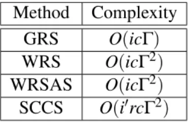
Method Complexity GRS O(icΓ) WRS O(icΓ2) WRSAS O(icΓ2) SCCS O(i0rcΓ2)

Table 1: The complexity of the algorithms presented.

O(icΓ2). A limit on the number of feature subsets inΓwould reduce the complexity but that method is not used in this algorithm.

The complexity of WRSAS does not increase the complexity of WRS because the only change is an addition during the computation of the normalization term.

The complexity of SCCS is similar to the others but the number of iterations is replaced as follows: i=i0rwherei0is the number of iterations per reduction andris the number of reductions. The true number of iterations are represented by the producti0r, as they together are the main control loops in the algorithm.

To move beyond a greedy algorithm the complexity is increased byΓto account for computing thenormfunction. The complexity of the last 3 algorithms is the same. SCCS splitsiintoi0andrbut effectively we achieve better results without increasing the total number of iterations.

CHAPTER 3

EXPERIMENTS

This algorithm is evaluated on a portion of the HRSC nadir panchromatic image

h0905 0000 from [HRS], taken by the Mars Express spacecraft. This image is located in the Xanthe Terra, centered on Nanedi Vallis and covers mostly Noachian terrain on Mars. Two smaller datasets are created from this image and shown in Figure 6. The selected image has the resolution of 12.5 meters/pixel and a size of 11,560,000 pixels (4 tiles x 1700 x 1700 ) pixels. A domain expert manually marked 1,269 craters for this image to be used as the ground truth to which the results of auto-detection are compared. The image represents a significant challenge to automatic crater detection algorithms. It covers terrain having spatially variable morphology and it’s contrast is rather poor. To make it easier for this work to be repeated the internal names of the datasets are used. The dataset can be found at the University of Massachusetts Boston Knowledge Discovery Lab’s website1

We detect craters larger than 16 pixels (200 m in the h0905 0000 image) but no larger than 400 pixels (5,000 m in the h0905 0000 image). Large craters have already been identified and smaller craters lack enough information to expect to be identified at this point.

Using the technique in Figure 7 originally described by [US09] and [BDS10] we can identify 2,404 crater candidates in our subdataset of h0905 0000. This preprocessing step allows us to avoid sliding window candidate generation which would generate a very large

Figure 6: Datasets A (left) and B (right) are composed of 2 square sections of the HRSC nadir panchromatic image h0905 0000 from [HRS]. The ground truth is overlaid on the image in white. The tile names from our public datasets are as follows. Dataset A is composed of 2 24 and 2 25 while Dataset B is composed of 3 24 and 3 25

number of candidates. This tradeoff however causes some craters to be unrecoverable in later phases. In generating our dataset of 1,269 craters, 72 are lost. We accept this loss in order to significatly reduce the number of candidates needed to be processed.

Figure 7: Left: Crater detection pipeline, Right: Haar Masks used to extract features from images.

Each crater candidate image block is normalized to a standard scale of 48 pixels before we extract features from the image in order to have a uniform feature addressing scheme.

To extract features from these images we use Haar feature masks. Haar features capture contrast information which gives insight into the texture of the crater. Other methods such as high or low pass filters do not encapsulate this contast information and provide less information per feature. Each of the nine kinds of Haar image masks as described by [VJ04], shown in Figure 7, probes the normalized image block in four different scales of 12 pixels, 24 pixels, 36 pixels, and 48 pixels, with a step of a third of the mask size (meaning 2/3 overlap), returning 121 scale independent feature values. In total 1,089 Haar-like features are extracted.

Haar features are described using feature masks that specify white and black regions. The masks are overlaid on the crater image and the sum of each region’s pixel values are calculated then the difference is taken. In Figure 7 the masks are shown as well as the full

Figure 8: This figure shows the impact of the size of the initial pool of features subsets on the resulting F1 value of the final subset. The average of over 5000 runs of the algorithm are presented. For this experiment each run consisted of 1000 iterations, a population of 10 subsets, and a mutation rate of 1% Top: Dataset A, Bottom: Dataset B

pipeline used and described by [DSM11]. The features extracted depend on the image format for precision and size. Haar features can be optimized for speed using an technique discussed by [VJ04] that allows for O(1) calculations of Haar features from an image that has had a corresponding Integral Image computed.

During these experiments lines are labeled with the convention Method-Dataset. For example the algorithm Greedy Random Search run on dataset B would be notated as GRS-B.

A challenge of experimenting with these algorithms is finding their optimal

parameters. This section will analyze the mutation rate, number of iterations, maximum number of feature subsets accumulated, the number of feature subsets generated for the initial pool, and the number of maximum cardinality corrections made.

To evaluate the proposed algorithms. Haar features are used in combination with a Bayesian classifier. The naive use of all features by the Bayesian classifier causes it to react drastically to changes in features. This gives the algorithm more feedback and allows it to acknowledge success or failure when removing or adding image features into the child subset.

Theinitial pool sizeis the set of feature subsets that are given to the algorithm to start the process. The minimum number of features is two. Values from 10 to 700 are used over 1000 iterations at 1% mutation to determine the optimal value. There does not seem to be any significant trend with this parameter in Figure 8 because the fluctuation is minimal and does not appear to have a significant trend.

Themaximum size ofϒvariable is the limit of feature subsets that will be maintained in memory during the program execution. It is also called the population. This is only used for WRS and WRSAS. Values were sampled from 3 to 1000 during 10000 iterations at 1% mutation and concluded no significant fluctuation or trend. The experiments start at 3 because otherwise it is GRS. GRS keeps only 2 feature subsets in memory so there is no collection of feature subsets to vary. However this value must be chosen greater than 2 so these algorithms differ from greedy search.

Amutationrate needs to be chosen for GRS, WRS, and WRSAS. The rate is the percentage of the feature subset that will be randomly turned on or off. A constant percentage is used for every iteration. The elements that are changed are randomly selected each iteration. Experiments were performed using 1000 iterations, 10 randomly generated initial feature subsets, and a Naive Bayes Classifier. In Figure 9 it appears that the best mutation rate is around 1%. If too much of the chromosome is mutated the fitness of the subsets suffers but if there is no mutation then the algorithm are missing out on a possible gain in fitness. Higher mutation rates also have a negative effect on the subset size, increasing it with higher mutation rates.

To establish insight into the runtime cardinality bound process of the SCCS algorithm, the average bound reductions are plotted in Figure 10. In this figure the best chromosome cardinalities are averaged across over 100 samples while varying the number of reductions at increments of 1 using intervals of 1000 iterations between reductions. It is clear that

Figure 9: Average Percentage of Mutation verses fitness and resulting subset size. Left: fitness, Right: resulting subset size. The average of over 5000 runs of the algorithm are presented. The parameters for these experiments were Iterations=1000, Population=10, and Initial Pool=10. Top: Dataset A, Bottom: Dataset B

more features are removed when using the shrinking cardinality chromosome than when it is not used. The bound appears to exponentially decrease and approach an asymptote as the number of reductions increases. The most significant decrease in bound is the first reduction. This is simply the mean of the highest performing subsets generated without any reductions. This is significant because the algorithm only shrinks the bound when the size of the subsets that achieve the same or better fitness use less image features than their parents. These continued reductions imply that bounding the maximum cardinality does in fact influence the reproductive process.

Figure 10: The average bound size afterx reductions on the datasets. The starting bound, not shown, is the total numbers of features, 1089.

To examine the shrinking cardinality chromosome algorithm, the method is used in conjunction with the genetic search methods presented in this paper to increase their performance. The only new variable is the number ofreductions. This method has an optimal mutation rate that differs from the selection methods presented. The mutation rate that causes the previous algorithms to perform optimally as well as the trend observed for mutation do not apply once SCCS is used. We will continue to use the previous initial pool value of 10 subsets, and a population limit of 10 subsets.

To explore the mutation rate, the previous experiment is modified to run with SCCS and a reduction rate of 5 reductions. 5 reductions allows the algorithm to take advantage of SCCS’s bounded searching while not requiring long runtimes. Figure 11 clearly shows a different trend than the previous analysis of mutation rates. In this plot, instead of reducing F1 as the mutation rate grows the opposite occurs. Also the subset size growth is not linear anymore. Using these experiments the mutation rate of 20% is chosen balance fitness with subset size.

Figure 11: Mutation rate effect on subset fitness using the SCCS method configured with 5 reduction steps of 1000 iterations each, and a population and initial pool of 10.Top: Dataset A, Bottom: Dataset B

Figure 12 presents 10-fold cross validation of each selection algorithm in this paper compared to it’s modified version using SCCS. Each column is a dataset and each row is a selection method run on a dataset. The results show that SCCS only outperforms the other presented algorithms on Dataset B. This is interesting because in Figure 4 it appeared that Dataset A would benefit greater from smaller subset sizes rather than Dataset B as it seems to not require small subsets to achieve a high F1 score.

For the situations that SCCS achieved higher F1 scores the results are immediate after only 2000 iterations. The differences in F1 between SCCS and non-SCCS method begins to converge as the iterations reach 15000. On the other hand in the situations that it did not

Figure 12: Comparison between the genetic feature selection process without correcting the maximum size of the chromosome and a process that corrects the maximum size to be the mean size of the top performing chromosomes.

achieve higher F1 scores it seems to remain at the same F1 level while the other algorithms presented continue to increase.

The overall results for each method are presented in Figure 13. These are the best mean values for each specific method between 1 and 1500 iterations. Naive Bayes is shown using all features to achieve the lowest F1 score. Naive Bayes is not only used

Figure 13: Overall results of all methods presented during 10-fold cross validation. Left: Best average F1 scores, Right:Best average subset sizes, Top: Dataset A, Bottom: Dataset B

internally for the presented feature selection methods but is also the classifier built using the subset generated by these methods. The subset size for Naive Bayes is 1089 because it utilizes all features extracted from the candidate images. AdaBoost is used as a baseline for comparison. AdaBoost was run using a Decision Stump classifier, 10 iterations, a weight threshold of 100, and no resampling.

For Dataset A the increase from Naive Bayes using all features to WRSAS selected features is almost 9% for F1 score. The best average subset size is a little more than 18 image features when using SCCS and WRSAS. With these methods we can achieve higher accuracy with only 1.6% of the original crater image features.

For Dataset B the increase in F1 is about 5% over Naive Bayes with all features when using WRSAS and SCCS selected features. Using SCCS does not result in a smaller subset but WRSAS alone results in an average subset size of only 21 image features. Our

methods are able to achieve better results using only 1.9% of the original crater image features.

Figure 15 shows the classification results of the SCCS method trained with half of dataset A and B respectively and then used to classify the other halves. These datasets generated 1,269 candidates that were able to be processed at 0.5ms/candidate.

Classifier training costs an average of 3msper instance with 1089 features. The time growth due to features is shown in Figure 14. All timing is based off a single thread of a 3.20GHz Intel i7 processor running 64-bit Linux.

Figure 14: Here the number of input features to the SCCS method is varied from 50 to 1000 and binned into groups of 100. The average time required to perform the feature selection and train the classifier is shown over 500 experiments. SCCS is configured with 15 reductions with 1000 iterations each. The bottom half of dataset B (containing 727 instances) is used as a training set.

Figure 15: Here SCCS is used with 15 reductions of 1000 iterations each. A classifier for each half of the dataset is built using the other half (top/bottom). Correct detections are shown as a white circle. False detections, both positive and negative are shown as a red square. We achieve 0.844 accuracy on Dataset A and 0.888 on Dataset B. Classification of each instance took 0.5ms.

CHAPTER 4

CONCLUSION

This paper presented four feature selection algorithms that increase the classification ability of the Naive Bayes classifier. This is necessary because during applications of machine learning the classifier is presented with discriminate and indiscriminate features which may be irrelevant or redundant. By removing these irrelevant or redundant features classification speed and ability can improve. The algorithms presented have shown their ability to boost the classification ability of a classifier on a real world large scale dataset for the task of automatic crater detection which is currently in demand by the planetary science community. We specifically present an algorithm that, using a property of crater image datasets, simultaneously reduces the subset size and increases the classification performance.

Acknowledgment

This research was supported in part by NASA Grant NNX09AK86G and NSF Grant 1062749.

REFERENCE LIST

[AD91] H. Almuallim and T. G Dietterich. “Efficient algorithms for identifying relevant features.” InProceedings of the Ninth Canadian Conference on Artificial Intelligence, pp. 38–45, 1991.

[BDS10] L. Bandeira, W. Ding, and T. F Stepinski. “Automatic Detection of Sub-km Craters Using Shape and Texture Information.” InProceedings of the 41st Lunar and Planetary Science Conference, The Woodlands, Texas, March 2010. [BDS11] L. Bandeira, W. Ding, and T. F. Stepinski. “Detection of sub-kilometer craters

in high resolution planetary images using shape and texture features.”

Advances in Space Research, 2011.

[BHV95] J. Bala, J. Huang, H. Vafaie, K. DeJong, and H. Wechsler. “Hybrid learning using genetic algorithms and decision trees for pattern classification.” In

International Joint Conference on Artificial Intelligence, volume 14, pp. 719–724, 1995.

[BPA03] S. Brumby, C. Plesko, and E. Asphaug. “Evolving automated feature extraction algorithms for planetary science.” InISPRS WG IV/9:

Extraterrestrial Mapping WorkshopAdvances in Planetary Mapping, 2003. [BSP07] L Bandeira, Jose Saraiva, and Pedro Pina. “Impact Crater Recognition on Mars

Based on a Probability Volume Created by Template Matching.” IEEE Transactions on Geoscience and Remote Sensing,45(12):4008–4015, December 2007.

[CF94] R. Caruana and D. Freitag. “Greedy attribute selection.” InProceedings of the Eleventh International Conference on Machine Learning, p. 2836, 1994. [CJM03] Y. Cheng, A. E Johnson, L. H Matthies, and C. F Olson. “Optical landmark

detection for spacecraft navigation.” Advances in the Astronautical Sciences,

114:1785–1803, 2003.

[CLD11] Joseph Paul Cohen, Siyi Liu, and Wei Ding. “Genetically Enhanced Feature Selection of Discriminative Planetary Crater Image Features.” InProceedings of the The 24th Australasian Joint Conference on Artificial Intelligence, Perth, Western Australia, December 2011.

[CS96] K. J Cherkauer and J. W Shavlik. “Growing simpler decision trees to facilitate knowledge discovery.” InProceedings of the Second International Conference on Knowledge Discovery and Data Mining, pp. 315–318, 1996.

[DA10] Mert Degirmenci and Shatlyk Ashyralyyev. “Impact Crater Detection on Mars Digital Elevation and Image Model.” Middle East Technical University, 2010. [DK82] P. A Devijver and J. Kittler.Pattern recognition: A statistical approach.

Prentice/Hall International, 1982.

[DSM11] W. Ding, T. F Stepinski, Y. Mu, L. Bandeira, R. Ricardo, Y. Wu, Z. Lu, T. Cao, and X. Wu. “Sub-kilometer crater discovery with boosting and transfer

learning.” ACM Transactions on Intelligent Systems and Technology,2(4), July 2011.

[Hal99] M. A Hall. Correlation-based feature selection for machine learning. PhD thesis, Citeseer, 1999.

[HIK02] R. Honda, Y. Iijima, and O. Konishi. “Mining of topographic feature from heterogeneous imagery and its application to lunar craters.” Progress in Discovery Science, pp. 27–44, 2002.

[HiR] HiRISE. “HiRISE|High Resolution Imaging Science Experiment.” http://hirise.lpl.arizona.edu/.

[HRS] HRSC. “HRSC Data Browser.”

http://europlanet.dlr.de/node/index.php?id=209, 2010.

[ILE00] I. Inza, P. Larranaga, R. Etxeberria, and B. Sierra. “Feature subset selection by Bayesian network-based optimization.” Artificial Intelligence,

123(1-2):157–184, 2000.

[JKP94] G. H John, R. Kohavi, and K. Pfleger. “Irrelevant features and the subset selection problem.” InProceedings of the eleventh international conference on machine learning, volume 129, pp. 121–129, 1994.

[KJ97] R. Kohavi and G.H. John. “Wrappers for feature subset selection.” Artificial intelligence,97(1-2):273–324, 1997.

[KMV05] J. R Kim, J. Muller, S. Van Gasselt, J. G Morley, and G. Neukum. “Automated crater detection, a new tool for Mars cartography and chronology.”

Photogrammetric engineering and remote sensing,71(10):1205, 2005.

[KS96] D. Koller and M. Sahami. “Toward optimal feature selection.” InProceedings of the Thirteenth International Conference on Machine Learning, pp. 284–292, San Francisco, CA, 1996.

[LDC11] Siyi Liu, Wei Ding, Joseph Paul Cohen, Dan Simovici, and Tomasz F.

Stepinski. “Bernoulli Trials Based Feature Selection for Crater Detection.” In

Proceedings of the 19th ACM SIGSPATIAL International Conference on Advances in Geographic Information Systems, Chicago, Illinois, November 2011. ACM.

[Mic03] G.G. Michael. “Coordinate registration by automated crater recognition.”

Planetary and Space Science,51(910):563–568, August 2003.

[Pik80] R.J. Pike. “Control of crater morphology by gravity and target type-Mars, earth, moon.” InLunar and Planetary Science Conference Proceedings, volume 11, p. 21592189, 1980.

[POP98] C. P Papageorgiou, M. Oren, and T. Poggio. “A general framework for object detection.” Center for Biological and Computational Learning Artificial Intelligence Laboratory, 1998.

[Rus09] Stuart Russell. Artificial intelligence. Pearson Education, Upper Saddle River N.J. ;;Harlow, 3rd ed. edition, 2009.

[SL08] G. Salamuniccar and S. Loncaric. “Open framework for objective evaluation of crater detection algorithms with first test-field subsystem based on MOLA data.” Advances in Space Research,42(1):6–19, July 2008.

[SL10] Goran Salamuniccar and Sven Loncaric. “Method for crater detection from Martian digital topography data using gradient value/orientation,

morphometry, vote analysis, slip tuning, and calibration.” Geoscience and Remote Sensing, IEEE Transactions on,48(5):23172329, 2010.

[SLM12] Goran Salamunicar, Sven Lonari, and Erwan Mazarico. “LU60645GT and MA132843GT catalogues of Lunar and Martian impact craters developed using a Crater Shape-based interpolation crater detection algorithm for

topography data.” Planetary and Space Science,60(1):236–247, January 2012. [SLP11] G. Salamuniccar, S. Loncaric, Pedro Pina, Louren\cco Bandeira, and Jos

Saraiva. “Integrated crater detection algorithm and systematic cataloging of phobos craters.” InImage and Signal Processing and Analysis (ISPA), 2011 7th International Symposium on, p. 591596, 2011.

[SU04] David J Stracuzzi and Paul E Utgoff. “Randomized Variable Elimination.” J. Mach. Learn. Res.,5:13311362, December 2004. ACM ID: 1044704.

[SU08] T. F. Stepinski and E. R. Urbach. “Completion of the first automatic survey of craters on Mars.” InProceedings of the 11th Mars Crater Consortium meeting, US Geological Survey in Flagstaff-AZ, 2008.

[Tan86] K. L Tanaka. “The Stratigraphy of Mars.” InProceedings of the Seventeenth Lunar and Planetary Science Conference, Houston, Texas, 1986.

[US09] E. R Urbach and T. F Stepinski. “Automatic detection of sub-km craters in high resolution planetary images.” Planetary and Space Science,

57(7):880–887, 2009.

[VD95] H. Vafaie and K. De Jong. “Genetic algorithms as a tool for restructuring feature space representations.” InTools with Artificial Intelligence, 1995. Proceedings., Seventh International Conference on, p. 811, 1995.

[VJ04] P. Viola and M. J Jones. “Robust real-time face detection.” International journal of computer vision,57(2):137–154, 2004.