Multi-Label Classification Using Higher-Order Label Clusters

Student Work

12-2018

Multi-Label Classification Using Higher-Order

Label Clusters

Dilanga Lakshitha Bandara Abeyrathna Galapita Mudiyanselage

University of Nebraska at Omaha

Follow this and additional works at:https://digitalcommons.unomaha.edu/studentwork Part of theComputer Sciences Commons

This Thesis is brought to you for free and open access by

DigitalCommons@UNO. It has been accepted for inclusion in Student Work by an authorized administrator of DigitalCommons@UNO. For more information, please [email protected].

Recommended Citation

Abeyrathna, Dilanga Lakshitha Bandara Galapita Mudiyanselage, "Multi-Label Classification Using Higher-Order Label Clusters" (2018).Student Work. 2921.

A Thesis Presented to the

Department of Computer Science, and the

Faculty of the Graduate College University of Nebraska

In Partial Fulfillment

of the Requirements for the Degree Master of Science in Computer Science

University of Nebraska at Omaha by

Dilanga Lakshitha Bandara Abeyrathna, Galapita Mudiyanselage December, 2018

Supervisory Committee: Dr. Parvathi Chundi Dr. Mahadevan Subramaniam

ProQuest Number:

All rights reserved

INFORMATION TO ALL USERS

The quality of this reproduction is dependent upon the quality of the copy submitted.

In the unlikely event that the author did not send a complete manuscript

and there are missing pages, these will be noted. Also, if material had to be removed, a note will indicate the deletion.

ProQuest

Published by ProQuest LLC ( ). Copyright of the Dissertation is held by the Author.

All rights reserved.

This work is protected against unauthorized copying under Title 17, United States Code Microform Edition © ProQuest LLC.

ProQuest LLC.

789 East Eisenhower Parkway P.O. Box 1346

Ann Arbor, MI 48106 - 1346 10982898

10982898

Dilanga Galapita Mudiyanselage, M.S. University of Nebraska, 2018 Adviser: Dr. Parvathi Chundi

Multi-label classification (MLC) is one of the major classification approaches in the context of data mining where each instance in the dataset is annotated with a set of labels. The nature of multiple labels associated with one instance often demands higher computational power compared to conventional single-label classification tasks. A multi-label classification is often simplified by decomposing the task into single-label classification which ignores correlations among labels. Incorporating label correlations into classification task can be hard since correlations may be missing, or may exist among a pair or a large subset of labels. In this study, a novel MLC approach is introduced calledMulti-Label Classification with Label Clusters (MLC–LC), which incorporates label correlations into a multi-label learning task using label clusters. MLC–LCuses the well-knownCover-coefficient based Clustering Methodology (C3_M)to

partition the set of labels into clusters and then employs either thebinary relevanceor the label powersetmethod to learn a classifier for each label cluster independently. A test instance is given to each of the classifiers and the label predictions are unioned to obtain a multi-label assignment. TheC3_{Mmethod is especially suited for constructing label}

clusters since the number of clusters appropriate for a label set as well the initial cluster seeds are automatically computed from the data set. The predictive of MLC–LCis compared with many of the matured and well known multi-label classification techniques on a wide variety of data sets. In all experimental settings,MLC–LC outperformed the other algorithms.

COPYRIGHT

ACKNOWLEDGMENTS

Firstly, I am very grateful for my advisor Dr. Parvathi Chundi, for all support and help she bestowed on me. Dr. Chundi extended her support not only to improve my research but funded my master’s studies as a Graduate Research Assistant. This

assistantship gave me a scope to extend my research work and gave me an opportunity to work in multiple projects which helped me gain enormous knowledge and opened me to a wide variety of new areas in technology. I express my deep gratitude for Dr. Chundi for the educational, financial and moral support from the beginning of my degree.

I would like to acknowledge Dr. Mahadevan Subramaniam, member of the

supervisory committee who I worked closely with, has always been a pillar of strength all through my master’s journey. I am grateful that I got an opportunity to work with Dr. Subramaniam, who has always been enthusiastically motivating me with not only my research but also guided me through tough times in my personal life and has been a great moral support. I would like to thank Dr. Abhishek Parakh, member of my

supervisory committee for his continuous support for my research and actively involving in improving my research.

I am thankful for my mate Ravi Teja, who helped me with the implementation ofC3

clustering in Java that was greatly helpful in my research. I would like to thank my fellow students Srikanth Vadla, Vidya Bommanapally and Shane McDermott for helping me in several ways and providing me with the gaming platformQuasimwhere I could readily apply for my research work.

My special thanks to Holland Computer Centre Resources and Crew, which is the main source of results in my research project, without which my thesis could have been very difficult.

This accomplishment would not have been possible without all your help. My sincere gratitude to all of you for having confidence in me and supporting me all through. Thank you!

Contents

List of Figures v

List of Tables vii

1: Introduction 1

1.1 Overview . . . 1

1.2 Aims and Objectives . . . 3

1.3 Structure of chapters . . . 5

2: Literature Review 6 2.1 Learning Algorithms . . . 6

2.2 Evaluation Matrices . . . 9

2.2.1 Label-based evaluation matrices . . . 10

2.2.2 Example-based evaluation matrices. . . 11

2.3 Cover Coefficient Clustering method . . . 12

3: METHODOLOGY 15 3.1 C3_MClustering . . . 15

3.2 MLC-LC . . . 19

3.3 Computational Complexity of MLC–LC . . . 21

4.1 Data Sets . . . 22

4.2 Results of Experiments . . . 25

4.2.1 Classification Accuracy of MLC–LC . . . 26

4.2.2 Classification Accuracy with Different Training Set Sizes . . . 32

4.2.3 Classification with Different Label Clustering Algorithms . . . 32

5: CONCLUSIONS AND FUTURE WORK 41

References 43

List of Figures

1.1 Beach scene . . . 2

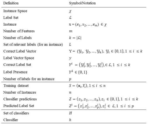
2.1 Symbols and Notations Used in this report . . . 7

2.2 BR method . . . 7

2.3 LP method . . . 8

2.4 RAkEL method . . . 8

2.5 Evaluation matrices categorization . . . 10

2.6 D matrix representing document-term matrix . . . 13

3.1 E matrix representing label assignment . . . 16

3.2 The Cover Co-efficient Matrix . . . 16

3.3 Non-overlapped label set training process . . . 20

3.4 Classification process . . . 21

4.1 micro-F1, macro-F1 and hamming Loss scores for 66% random sampling training set. Experimental results (mean±std) on data. ↑(↓) indicates the larger (smaller), the better . . . 27

4.2 micro-F1, macro-F1 and hamming Loss scores for 66% stratified sampling training set. Experimental results (mean±std) on data. ↑(↓) indicates the larger (smaller), the better . . . 28

4.3 Ranking of MLC methods according to their micro-F1, macro-F1 and ham-ming loss scores for 66% random sampling training set . . . 29

4.4 Ranking of MLC algorithms Based on micro-F1, macro-F1and hamming Loss

score for stratified sampling . . . 30

4.5 F1scores for Yeast data set with 66% random sampling training set and 34%

testing set . . . 31

4.6 micro-F1, macro-F1Scores and hamming loss values of Different MLC

meth-ods for Training Set Sizes 70% and Testing set size 30%. . . 33

4.7 micro-F1, macro-F1Scores and hamming loss values of Different MLC

meth-ods for Training Set Sizes 50% and Testing set size 50%. . . 34

4.8 micro-F1, macro-F1scores and hamming loss values of Different MLC

meth-ods for Training Set Sizes 30% and Testing set size 70%. . . 35

4.9 (a) Micro-F1and (b) Macro-F1scores of theMLC–LCClassifiers Obtained from

List of Tables

4.1 Multi-label Data Sets . . . 23

Chapter 1

Introduction

1.1

Overview

According to the machine learning literature, there are three main classification

categories namelybinary,multi-class, andmulti-labelclassification. This categorization is mainly based on the number of labels assigned to each instance in the dataset. When instances are associated with single label from a set which has two outcomes

positive/negative (or true/false) can be recognized as binary classification where as in Multi- class classification problems each instance in the dataset annotated with single label from a finite set of outcomes. As an example, detecting a mail whether it is spam or not (true/ false) is a binary classification problem and categorizing Iris flower into either an Iris Setosa, Iris Versicolour, or Iris Virginica is a multi-class classification problem. However, these two classification problems are commonly recognized asSingle label classification problem as final annotation is only having single label. Both of these classification problems learn a classifier (or a classifier ensemble) using a set of training instances and then use the classifier (or the ensemble) to assign a single label to a new (or a test) instance.

classification problem where each instance is associated with a set of labels. For example, according to the single label classification, Figure1.1can be annotated beach where as Multi-label classification approach can annotate the same image with beach, blue, water, chair, tree, sea for the image. Further, Multi-label classification problems are common in real-world applications. For example, a given email message may be labeled as both personalandimportant. Similarly, a news article may be classified asreligious,conservative, andliberal. Each input instance in a multi-label data set may be labeled with more than one label. Hence, the challenge is to annotate newer instances with multiple appropriate labels as possible.

Figure 1.1: Beach scene

Mainly there are two approaches to tackle multi-label classification problem known as problem transformation method and algorithm adaptation method. Problem

transformation method transfers a multi-label problem into a set of single label

classification problems so that they can be handled by a set of single-label classifiers and union the outputs to retrieve the final solution. One simple problem transformation

approach for predicting multiple labels for a given instance is to train a binary classifier for each label separately, which is also known as thebinary relevance (BR)method1

(Figure2.2). A test instance is given to each binary classifier to find all appropriate labels. However, using binary classification approach to solve a multi-label classification problem has severe drawback that it ignores the correlations among labels. For example, if an image (Ex: Figure1.1) is labeled withwater, it is more likely that it is labeled with blue. As these set of binary classifiers executes mutually exclusive manner there is no way to identify or preserve label dependencies. One way to incorporate correlations among labels is to treat each label combination as a distinct label and transform multi-label classification problem into multi-class classification problem, known as thelabel powerset (LP)method.1Here, each class label is a boolean vector of the size of all possible label set. If an instance contains a particular label, then the label in the boolean vector is set to 1, otherwise, it is set to 0. When a new instance is given to this classifier, it returns one boolean vector with possible label values set to 1. Though it is true that this approach can retrieve the complete label correlations, the upper bound of the combinations are

exponential (2n_{) and class imbalance issues can occur as the number of instances for}

each distinct class label may be sparse.

1.2

Aims and Objectives

Label correlation is one of the major criteria which should preserve while building a multi-label classifier yet it can be challenging with the computational complexities.2_Cost

of the classification task could vary from linear to an exponential with the number of possible labels. Not only the training task of the multi-label classification task but also a prediction for a new instance takes extra time as there could be a higher number of annotations to be done. Therefore, the issue of managing the accuracy of multi-label classification while preserving the label correlations has received a lot of attention. Some

of the previous studies3_{focused on categorizing label correlation strategies into three}

main categories as follows.

• Thefirst-order strategy: label correlations among labels are totally ignored and consider multi-label classification problem as a number of independent binary classification problems (Ex : BR method).

• TheSecond-order strategy: computes pairwise relations among labels to distinguish between relevant and non-relevant labels or to identify co-occurrences among labels.4–6

• TheHigher-order strategies: considers all possible correlations between all other labels on one label.2,7

This study is to incorporate a higher-order strategy for capturing label correlations in a multi-label data set and build multi-label classifiers that preserve the higher-order label correlations. The proposed method, which named asMulti-Label Classification

with Label Clusters (MLC–LC)first partitions the set of labels into clusters based on how

they co-occur in data set. Then employee two matured problem transformation to classify each and every cluster partitions depending on the size of the partition.

However, the clustering method used for this study was well-knownCover-Coefficient

Based Clustering Methodology (C3M)that computes the label clusters by identifying

labels that occur in many records in the data set. The co-occurrence pattern of labels is used byC3_{Mto compute the number of clusters sufficient for the data set as well the}

initial seeds (centroids) of these clusters. This unique feature ofC3_{M is exploited to}

compute label clusters where the label correlations are captured effectively. The number of classifiers in the proposed approach is the same as the number of label clusters generated using theC3M method, which tends to be significantly smaller than the

number of labels.8_{Consequently, the number of classifiers that need to be trained and}

The main contributions of the study are as follows –

• Proposed a simple, yet novel, a multi-label classification called theMLC–LCmethod that first partitions the label set into groups of correlated labels and trains an LP classifier for each label cluster separately.

• The predictive performance of MLC–LCmethod was compared with that of several established MLC methods such as the RAkELd, RAkELo, HOMER, LP, and BR on a range of diverse data sets. Our method achieved superior performance in almost all experimental scenarios for all the data sets.

• MLC–LCalso outperformed the established MLC methods even for smaller training set sizes.

1.3

Structure of chapters

A review of related work is presented in chapter 2. The multi-label techniques, evaluation and validation measures are discussed in chapter 3. Chapter 4 describes the design and implementation of the experimental environment and results. The dissertation

concludes with chapter 5, which summarizes the key findings and discusses avenues for future work.

Chapter 2

Literature Review

2.1

Learning Algorithms

Multi-label classification approaches can be mainly categorized into algorithm

adaptation methods and problem transformation methods.1,9,10_{Algorithm adaptation}

methods extend a specific learning algorithm in order to handle multi-label classification problem directly whereas problem transformation approaches convert a multi-label classification problem into several classification or regression problems such as binary classification or multi-class classification. Several methods have been proposed to incorporate label correlations and feature-label correlations into learning in both algorithm adaptation as well as problem transformation methods.4,6,10–13 _{This study}

focuses on problem-transformation methods in this study sinceMLC–LCis also of the same category.

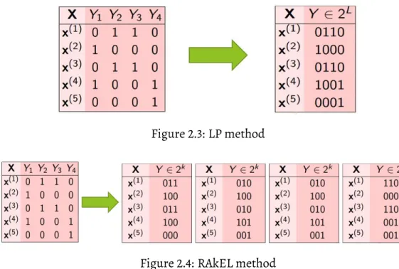
The Label Power set (LP) method14_{(Figure2.3)converts multi-label classification}

problem into a multi-class classification task while preserving label correlations by considering every label combination in the data set. However, it suffers from scalability and sparseness issues. Thepruned problem transformationmethod is proposed in15alleviate the scalability issues somewhat. TheRAndom k-labEL Set (RAkEL)approach7,11,14

Figure 2.1: Symbols and Notations Used in this report

Figure 2.2: BR method

(Figure2.4) is one of the popular approaches where the labels are randomly selected to form groups, each containingklabels (kis small compared to the total number of labels)

and an LP classifier is trained for each label set. A simple voting process determines the set of labels for each test instance.

Hullermeieret al16learnl(l−1)/2binary classifiers, one classifier for each pair of

Figure 2.3: LP method

Figure 2.4: RAkEL method

for which at least one of the labels in the pair is true, but not both. Furnkranzet alin6 introduced the notion of acalibration labelthat can be used to separate relevant and irrelevant labels predicted by pairwise classification methods to combine multi-class classification with ranking of labels.

There are also multi-label classification methods that incorporate higher-order label dependencies. A classic method is theclassifier chains17that generatelclassifiers by

incorporating the feature set of the data set given to each classifier by including the label associations assigned to each instance by the previously learned classifiers. Since the performance of a classifier chain may be influenced by the order in which labels are considered by the binary classifiers,probabilisticclassifier chains18have been proposed to predict the best chain ordering. In,3_{authors use association rules to compute the higher}

order label correlations which are used to select the best training examples. Then, cross-label uncertainty of predicted labels is used to extend the label set of the unseen examples which are then incorporated into the next learning step. Label correlations are also identified to combine predictions from multiple models in19_{to optimize for ranking}

TheMLC–LCmethodology is inspired by theRAkELmethods that generate groups of labels and learn an LP classifier for each group. The RAkELd method partitions the label set into equal size subsets, each containingklabels for some random integerkwhereas

RAkELo groups the labels into overlapping subsets.MLC–LCalso partitions the label set into subsets, however, the number of subsets and the size of each subset are determined by the correlations among labels existing in the data set. The cover-coefficient

methodology ofC3M is highly suited for finding the right number of label clusters and

the labels that should be grouped into each cluster. TheHOMER2algorithm for

multi-label classification also uses thebalanced clustering, specifically balancedK-means,

to distribute a label set intokgroups as evenly as possible. Then, it learns a hierarchy of

multi-label classifiers, each one learning a smaller label set compared to the classifiers at the previous level. Because of more balanced example distribution,HOMERalgorithm performed better than the BR method. The label clusters generated by our method MLC–LCmay not have balanced sizes. In fact, it is common for some of the label clusters to contain single labels and other label clusters may even have a dozen labels, all

depending on the data set. Despite this, the results of our experiments show superior predictive performance when compared to that of RAkELd, RAkELo, HOMER, BR, and LP methods.

2.2

Evaluation Matrices

Evaluation matrices are an important component in implementing and maintaining supervised learning model in order to estimate the performances and optimization. Accuracy, the area under the ORC curve (Receiver Operating Characteristic curve), precision and recall are used to evaluate supervised learning models for performances in general. However, evaluating multi-label classification problem is complex than single label classification problem. Multi-label classification performances should be evaluated

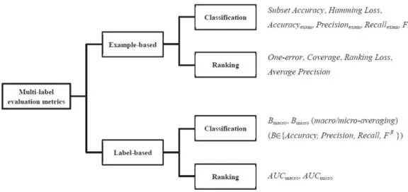
Figure 2.5: Evaluation matrices categorization

both in example wise as well as label wise. Therefore the two main categories of evaluation matrices are employed for multi-label classification. Example based evaluations consider the average prediction difference between actual data in test set where as label based evaluations consider label at a time and average overall label prediction performances (see Figure 2.5).

A classifier may assign all/none/few labels wrongly to a test instance during the prediction phase. Therefore, performance evaluation must take into account each label that was incorrectly predicted. It is also important to consider partial performances during the prediction. To cover most of these aspects, there are many evaluation

matrices introduced and most of the evaluation matrices are implemented to capture the correctness/loss in percentage.

2.2.1

Label-based evaluation matrices

• Macro / micro F1-measure

Recall thatLis the set of all labels of a multi-label data set. LetT ={(xi, Zi)}

(1≤i≤t) be a multi-label test set witht-test instances whereZi ⊆Lis the set of

true labels for theith_{instance. LetY}

multi-label classifier for theith_{instance. The precision of a multi-label classifier}

computes the ratio of relevant labels predicted by the classifier whereas recall measures the proportion of predicted labels that are relevant. AnF1-measureis

the harmonic mean of the precision and recall values. It is one of the most frequently used predictive performance-based evaluation metric in the field of classification.20_{The higher theF}

1-measure, better the performance.

precision=1 t Pt i=1 |Yi∩Zi| Zi recall=1 t Pt i=1 |Yi∩Zi| Yi .

There are many different evaluation metrics for multi-label classification (see1_).

We use the following three metrics, in order to compare our work with other popular methods.(1)Micro and MacroF1scores: Themicro-F1score is the

cumulativeF1-measure of over all labels inLwhereas themacro-F1score computes

theF1-measure for each label independently and averages these values over|L|to

obtain one final measure.1,10_{The formulas for computing the micro-F} 1and

macro-F1scores are given below. Here,Zij= 1 if theithinstance contains labeljas

one of the true labels, otherwise it is set to 0. Similarly,Y_ij= 1 if labeljis predicted

as true for theithinstance, otherwise it is set to 0.

micro-F1= 2P|L| j=1 Pt i=1Z j iY j i P|L| j=1 Pt i=1Z j i+ P|L| j=1 Pt i=1Y j i macro-F1=|L1| P|L| j=1 2Pt_i=1Z_ijY_ij P|L| j=1 Pt i=1Z j i+ P|L| j=1 Pt i=1Y j i

2.2.2

Example-based evaluation matrices

• Subset Accuracy: This matrix evaluates the fraction of exactly correct classified examples. However, subset accuracy evaluation matrix performs poorly when the label set size of the data set is really high as the evaluation criteria are

subsetaccuracy= 1 t Pt i=1 |Yi=Zi| |L|

• Hamming Loss (HL): Hamming loss is the most commonly used metric to evaluate the performance of a multi-label classifier. It is the size of the average symmetric difference between the set of true labels and the set of predicted labels of a data set. It is computed as follows. HL= 1 t Pt i=1 |Yi∆Zi| |L|

• One-error: One-error evaluates the fraction of examples such a way that, top-ranked label is not in the relevant label set.

• Coverage: This matrix evaluates how many instances should be travels through on average to cover all the relevant labels if the example.

All the above-mentioned evaluation matrices and other matrices have diverse methods to evaluate predictive and model generalization performances. It is important to select proper evaluation matrices to evaluate the interesting aspects of classification results and performances. However, to make evaluation phrase unbiased and precise, a classification system should be tested with multiple matrices to have a general overview of quality of classification performance from a different perspective.

2.3

Cover Coefficient Clustering method

According to the Information Retrieval System (IRS) concepts, document-based information retrievals mainly related to their terms. Similarity functions are used to determine the relevance of documents. As shown in Figure2.6document-term matrix can be built to process the queries. If the element of this matrix isdijwheremnumber of

documents andnnumber of terms then,dij = (1≤i≤m, 1≤j≤n),indicates the

D=           t1 t2 t3 t4 t5 t6 t7 d1 X X X X X X X d2 X X X X X X X d3 X X X X X X X d4 X X X X X X X d5 X X X X X X X d6 X X X X X X X          

Figure 2.6:D matrix representing document-term matrix

weighted. As clustering hypothesis is closely associated documents tend to be relevant to the given query.C3M method belongs to partitioning based clustering approach for

document based document retrieval.

This method is first proposed by Fazli-Can et.al8_{to cluster text documents based on}

word similarities.C3_{M method is a partitioning based clustering algorithm which}

chooses a set of documents as seeds and then all the non-seeds documents are assigned into seed documents so that the set of documents partitioned into clusters lead by seeds. The base concept ofC3M method is Cover Coefficient concept, which serves to identify

relationships among documents using document term matrices. Determination of the number of clusters (selecting cluster seeds using cluster seed power) and correlate the documents are done by Cover coefficient concepts. The resultant clustering is

guaranteed non-hierarchical clustering and seed based. The Cover Coefficient method determines document relationships of coverage and similarities in multi-dimensional space.C3_M method employees another matrix called C matrix to reflect the

above-mentioned coverage and similarities. C matrix is a Document-by-Document matrix which single element,Cij(1≤i,j≤m)indicates the probability of selecting any

term of difromdj.

C matrix has the information of the relationship between document-based on two-stage probability experiment. This experiment randomly select terms (t) from

documents (d) in two stages. In the first stage, if tkis the term selected randomly of

dj. However, to apply the Cover Coefficient concept, the entries of the D matrix must

satisfy the following two conditions. The first condition is no document can be empty which is each document must have at least one term. The second condition is, there should not be any term which does not appear in any document. Further, the C matrix have properties which can be listed as follows,

• Ci1+Ci2+Ci3+...+Cim= 1(All the rows should be sum up to 1)

• Fori6=j, 0≤cij ≤ciiandcii >0

• Ifcij = 0, thencji= 0and ifcji>0, thencji>0.

• If a term ofdiis appeared in another document, thenciiis always less than 1. If

not, it is equal to 1.

• cii =cjj =cij =cjiiff coupling and decoupling ofdianddj are equal.

C3_{M method has several characteristics which grab the attention for this study.}

Some of the characteristics ofC3_{Mare, its capability of determining the number of}

clusters suitable for a given document set, document distributions within clusters are uniform which ensures moderate cluster sizes (not too large in cluster size or not too large singleton clusters), Cover Coefficient concept guaranteed the independence of the order of the documents clustered in the clustering process. This method is further explained in detail in the methodology section including examples of how it is employed in this study.

Chapter 3

METHODOLOGY

3.1

C

3

M

Clustering

The proposed approach uses theC3_{Mclustering method}8_{to partition labels into clusters}

of potentially dependent labels. This section briefly describes the main steps ofC3_M

method with simple examples below. The input to the algorithm is anm×nBoolean

matrix,E, whose rows are indexed by the set of labels,L= {l−1,· · ·,lm}, and columns

are indexed by the elements of set of records,R= {r1,· · ·,rn}. If labelliis assigned to the

recordru,E(i,u) = 1. Theassignment profileof labelliis given by theithrow ofEand the

labeling profileof recordruis given by theuthcolumn ofE. The matrixEdoes not contain

any zero columns or zero rows1_{The output of the method is a clustering of labels with the}

number of clusters being automatically determined by the method. TheC3_Mmethod

uses a notion of coverage among labels to group them into clusters. The main steps of the

C3_Mmethod are given below.

Consider theEmatrix in Figure3.1with 6 labels and 7 records. Each row specifies the

labels that are assigned to the records. For instance, first row ofEdenotes that testl1is

1_{Note that no labels may assigned to a record leading to a zero column corresponding to that record.}

Such columns are converted to non-zero columns by assigning to an extra "all-zero" label. If a label is not assigned to any of the records, then the corresponding zero row and the label are removed fromEandL respectively. More details are provided in the next section.

E =           r1 r2 r3 r4 r5 r6 r7 l1 1 0 0 1 1 0 0 l2 1 1 0 0 1 0 1 l3 0 0 1 0 0 0 0 l4 1 1 0 1 0 1 0 l5 0 1 1 1 0 1 1 l6 1 1 0 1 1 1 0          

Figure 3.1:E matrix representing label assignment

C =           l1 l2 l3 l4 l5 l6 l1 0.278 0.194 0.000 0.167 0.083 0.278 l2 0.146 0.333 0.000 0.125 0.188 0.208 l3 0.000 0.000 0.500 0.000 0.500 0.000 l4 0.125 0.125 0.000 0.271 0.208 0.271 l5 0.050 0.150 0.100 0.167 0.366 0.167 l6 0.167 0.167 0.000 0.216 0.167 0.283          

Figure 3.2:The Cover Co-efficient Matrix assigned to recordsr1,r4, andr5.

Cover Coefficients: The first step ofC3_M method takes_Eas input and outputs an_m×

msquare matrixCindexed by the setL. The entries ofCdenote pairwisecover coefficients values among the labels. Thecover coefficientcijof a labelliwith respect to a labellj is the

probability that a recordrulabeled byliis also labeled bylj. Informally, the cover

coefficient of a label with respect to another denotes the extent to which the assignment profile of the first label is covered by that of the second one. Letαiandβuare the

reciprocals of the sum of the entries in theith_{row and theu}th_{column of theEmatrix}

respectively. The entrycij inCis obtained using

cij =αi×rij where rij = n

X

k=1

(Eik×βk×Ejk). (3.1)

Applying Equation (1) to theEmatrix of the previous example to obtain theCmatrix

depicted in Figure3.2. For instance,c14=α1×[(E11×β1×E41) + (E12×β2×E42) +· · ·

(1/4)×1) + (1×(1/3)×0) + (0×(1/3)×1) + (0×(1/4)×0)] = (1/3)×(1/4 + 1/4) = 0.167.

As mentioned in Chapter 2, the cover coefficient valuecijcan be determined using a

two-stage selection process –a) select a recordrkthat is assigned the labelli, andii)

select labelljfrom the labels assigned to that record. In Equation (1), the first step of

selecting a recordrkthat is assigned the labelliis given by the productαi×Eik. The

second step of arbitrarily selecting the labelljfrom all the labels that have been assigned

the recordrkis given by the productβk×Ejk. To determine the extent to which the

assignment profile ofliis covered by that oflj, it is needed to consider all the recordsr1,

· · ·,rnindexing theEmatrix and this is given by the sumrij (The sumrij is called the

row-coveringof rowiby the rowj).

Note that the computation of the entrycij uses assignment profiles of all the labels.

In particular, the value ofcijdoes not equal the ratio of the common number of records

assigned both the labels over the total number of records assigned labelli.

Partitioning Labels into Clusters: The second step of theC3M method takes the matrix Cas input and outputs the number of clusters and the cluster seeds. Each cluster in C3_{Mconsists of a group of labels that are covered maximally by the seed of that cluster.}

Cluster seeds are labels with distinguishing assignment profiles i.e., they are not likely to be covered by other labels. If a label has a distinguishing assignment profile then it is assigned to records that others are not assigned to, and hence its profile is unlikely to be covered by that of the others. The magnitude of a diagonal entry in theCmatrix is used

to identify labels with distinguishing profiles. The entryciiof theithrow is called the

decoupling coefficientof that row. The decoupling coefficient of theCmatrix,δ, is the mean

value of the decoupling coefficients of its rows. The number of clusters,nc, is:nc=m×δ.

: Continuing, with the running example, the decoupling coefficient for theCmatrix in

Figure3.2isδ= (0.278+0.333+0.500+0.271+0.366+0.283)/6=0.339. The estimated

number of clusters isnc=0.339×6'3.

decreases, the value of the diagonal entryciiincreases. The entry has a maximum value

of1when there is no sharing among the records assigned the labelliand assigned other

labels. In other words, if labellihas a high de-coupling coefficient, then it is not likely to

be covered by the other labels and hence is likely to create to its own cluster.It is easy to see that if every label has a high decoupling coefficient, thennc=mas desired since the

decoupling coefficient of theCmatrixδ= 1 in this case. It can also be verified that if all

the labels have identical profiles, thennc= 1.

Theclustering powerof labelliis

Pi =cii×(1−cii)× n

X

k=1

Eik (3.2)

The labels are ranked based on their clustering power and the topnclabels are

chosen as cluster seeds and are assigned to one cluster each. Ties are broken arbitrarily. A labelljis considered afalse seedand eliminated if there exists a seedliwhose cluster

seed power is within a specified thresholdδof that oflj and the coefficientscii,cjj,cji

andcij are sufficiently close, i.e., the magnitude of the pairwise difference ofcii,cjj,cij

andcjiare all within a specified threshold. In this case, the false seed is eliminated and

the next seed in the sorted order is picked. A threshold value of=0.001was used based

on the spread of the seed values in the experiments. Each remaining labelliinLis

assigned to a cluster whose seedljmaximally coversli, i.e.,cijis a maximal value, for1≤

j≤nc. If more than one seed maximally coverslithen the label is assigned to the cluster

whose maximal covering seed has the higher clustering power (ties are broken arbitrarily). If there exist labels inLthat cannot be assigned to any of the clusters

because none of the seeds cover them, i.e.,cij =0for all seed teststjthen these tests are

collected into an additionalragbagcluster, [(nc+1)thcluster].

The clustering powers for the six labels in our running example areP1= 0.602,P2=

andl6. The clusters obtained areC1= {l2},C2= {l3,l5},C3= {l1,l4,l6}.

3.2

MLC-LC

LetDbe a multi-label data set whereD= {(xi,Zi) | 1 ≤ i ≤ n}, wherexiis a feature

vector andZiis a subset of a set of labelsL= {l1,· · ·,lm}. First,MLC–LCprocessesDto

produce anm×nBoolean matrix,E, whose rows are indexed by the elements ofLand

the columns are indexed by the elements of the set of records,R= {r1,· · ·,rn}. If labelli

∈Zuand (xu,Zu)∈D, thenE(i,u) = 1, meaning that labelliis assigned to the recordru.

Theassignment profileof labelliis given by theithrow ofEand thelabeling profileof

recordruis given by theuthcolumn ofE. We assume that all the assignment and

labeling profiles inEto be non-zero, i.e., every record has at least one label assigned to it

and every label is assigned to at least one record. Next, the matrixEis input to theC3_M

clustering method to partition the label setLinto a disjoint set of label clustersL1,· · ·,

Lc.

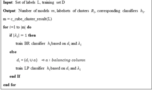
Then,MLC–LClearnscclassifiers, one for each label cluster. TheMLC–LCuses the BR method to learn the classifier for label clusters with a single label and uses the LP method otherwise. The training data for a classifier corresponding a singleton label clusterLk= {l} is obtained fromDby replacing each pair (xi,Zi) by the pair (xi,1) ifl

belongs toZiand is replaced by the pair (xi,0) otherwise. IfLkhas more than one label,

then we add a new labelaltoLk, the training data is obtained fromDby replacing each

pair (xi,Zi) by the pair (xi,Zi∩Lk). In cases whereZi∩Lk= {},(xi, Zi)is replaced by

(xi,{al}). It should be clear that the pair(xi,{al})is simply a placeholder for a feature

vectorxibeing assigned all zero values for each of the labels inLk. Note thatMLC–LC

generates at mostc/2new labels. However, this overhead is usually small since the

number of clustersc << m, the number of labels. Further, extra-label is added to

Figure 3.3: Non-overlapped label set training process

At the end of the training process,cclassifiers are obtained using the training data.

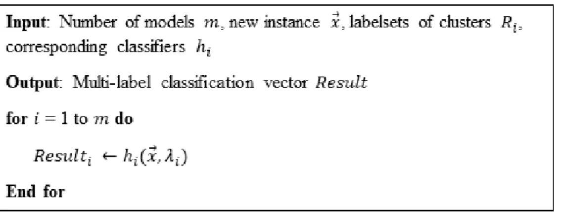
Some of these classifiers are BR classifiers and others LP classifiers. A test (or a previously unseen) instance is given to each classifier to get a label assignment. The resulting label assignments, which are disjoint, are simply unioned to obtain an assignment of multiple labels to the test instance. The new labels (i.e;al) added while

constructing the training set for LP classifiers are removed in the final assignment of labels to the test instances since eachalis just a place-holder to capture negative

instances with respect to a set of labels.

In the process of MLC-LC, clustered label sets(Ri)are classified using most popular

problem transformation methods, that is BR and LP methods appropriately. Resultant label clusters use to partition the multi-labeled dataset and run multi-label classification task for individual partitions. Partition sizes are dynamic as the label contained inRi

could be in the range of 1 to L. However, cluster sets have relatively small number of labels(λ << L)for most of the multi-label datasets, so that label dimension reduction is

done while preserving the label correlations. Hence both BR and LP methods perform efficiently on these smaller partitions of data sets.

Figure 3.4: Classification process

In the training process, single labeled clusters(|λ|= 1)are joined and compute BR

method. Clusters with more than one label(|λ|>1)train using LP method. Both BR and

LP methods use C5.0 decision tree algorithm on training.

3.3

Computational Complexity of MLC–LC

TheMLC–LCalgorithm has two phases – the label clustering phase and the training phase. The time complexity of theC3Malgorithm isO(m×xd×tgs)wheremis the

number of labels,xdis the average number of distinct records per label, andtgsis the

average number of seeds per record.8_Althoughx

dis bounded above byn(nis the

number of instances in the data set), it is much smaller in practice2_{. Also, the number of}

seeds is typically much smaller thanmand therefore,tgsis also a small value. Therefore,

C3_Mmethod can compute label clusters efficiently which was also observed in our

experimental set up. Once the label clusters are computed, the training phase learns as many BR/LP classifiers as the number of label clusters. If the complexity of a BR or a LP classifier isO(g(n))wherenis the size of the training set, and there arecclusters, then

the training phase takesO(cg(n))time to complete.

Chapter 4

EXPERIMENTAL SETUP

This section contains experimental setup in detail with environment used and experiment results. The main target of this experiment is to compareMLC–LC performances with respect to the matured and well-established methods (BR, LP, RAkELd, RAkELo, and HOMER) in the field of multi-label classification. Section4.1

describes the multi-label data sets, Section2.2contains the description of evaluation metrics used, and Section4.2is dedicated to results and discussion.

4.1

Data Sets

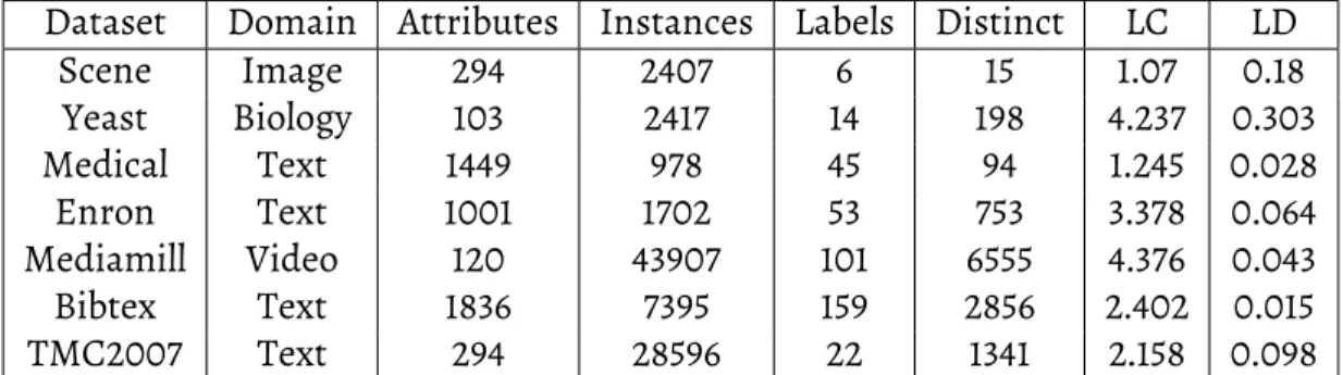
For these experiments, a variety of data sets from different domains are used. All the data sets used to conduct the experiment are listed in Figure4.1. The first column,Dataset, lists the name of the data set. Thedomaincolumn lists the domain the data collection related to. ColumnsInstances,Attributes, andLabelsshow the number of instances, number of attributes and number of labels respectively in the data set. Another important characteristic of a data set is the proportion of distinct label combinations listed in columnDistinct. Distinct label combinations capture the complexity of a labeling scheme.

LetDbe a multi-label data set consisting of|D|multi-label examples(xi, Zi)where

Dataset Domain Attributes Instances Labels Distinct LC LD Scene Image 294 2407 6 15 1.07 0.18 Yeast Biology 103 2417 14 198 4.237 0.303 Medical Text 1449 978 45 94 1.245 0.028 Enron Text 1001 1702 53 753 3.378 0.064 Mediamill Video 120 43907 101 6555 4.376 0.043 Bibtex Text 1836 7395 159 2856 2.402 0.015 TMC2007 Text 294 28596 22 1341 2.158 0.098

Table 4.1: Multi-label Data Sets

Label cardinality(LC) ofDis the average number of labels assigned to the examples inD.

It is also known as the standard measure of multi-labeled-ness. TheLabel density(LD) is the average number of labels of the examples inDdivided by|L|. The last two columns of

the table list these two measures.

LC(D)=_|D1_|P|D| i= 1|Zi| LD(D)= _|D1_|P|D| i= 1 |Zi| |L|

The Scene21_{data set consists of 2407 natural scene images annotated with up to 6}

concepts (beach, sunset, field, fall foliage, mountain and urban). Many images contain more than one scene and feature representation is based on spatial color moments of each image. The Yeast22_{data set consists of micro-array expressions and phylogenetic}

profiles for 2417 yeast genes. Functional classes from the Comprehensive (e.g. metabolism, energy, etc) from the top level of the functional catalog (FunCat) are annotated as 14 labels.

The TMC200723_{data set is a collection of text data related to aviation safety reports. The}

original data set contains 28596 safety reports in text form and 22 problem types that appear during flights annotated as labels. Text representation is based on Boolean bag-of-words method. However, in this experiment, the feature set of the TMC2007 data set was reduced to 500 most relevant features for consistent comparison with other methods and manageable computation.

The Medical24_{data set is another text-based data set consisting of documents with free}

text summaries, patient symptoms histories and prognoses, which were used to predict insurance codes. This data set consists of 978 clinical reports annotated with one or more of 45 disease codes. Enron25_{is another popular text-based multi-label data set which}

contains collection of email messages exchanged between Enron corporation employees. The number of email messages in the data set is 1702 and each email message is assigned multiple labels from a total of 53 topics.

The Mediamill data set26_{consists of 43907 video frames annotated with 101 labels (e.g.}

military, desert, basketball, etc). This data collection was part of the Mediamill challenge for automated detection of semantic concept in 2006. Video frames were represented as a set of 120 visual features. The Bibtex data set27_{consists of labels of the Bibtex and}

Bookmarks corresponds to tags assigned to publications and bookmarks respectively by users of the social bookmark and publication sharing system Bibsonomy. It contains 7395 bibtex entries from the BibSonomy.

As can be observed from Figure 4.1, the size of the label sets ranges from 6 to 159. Although the distinct label combinations are only a fraction of the possible exponential number of label combinations, the number of label combinations is still too high to learn a model for each distinct label combination (In case of Bibtex data set, the number of models needed would be 811). The label density values range from 0.015 for the Bibtex data set to 0.303 for the Yeast data set. This shows that our experiments included data sets where the training data set for a label combination might be sparse, as well as the data sets where the training data set may have a large number of training instances for each label combination.

All the data sets were pre-processed and available in the MLDRRpackage20except

the Scene data set that was obtained from Mulan data repository1_{, which was used in our}

experiments.

4.2

Results of Experiments

The implementation ofMLC–LCis mainly done in Java andRstatistical programming

language and is compared with some of the popular existing multi-label classification approaches. TheC3M algorithm was implemented in Java. TheC3M clustering of the

label sets of these sets resulted in 3 clusters for the Yeast data set, 31 clusters for the Medical data set, 15 clusters for the Enron data set, 19 clusters for the Mediamill data set, 9 clusters for the TMC2007 data set, 66 clusters for the Bibtex data set and 6 clusters for the Scene data set. Ragbag cluster was not generated for any of the data sets.

The classification was done inRusing the packages –utiml(Utilities for Multi-Label Learning)28_{andmldr(Exploratory Data Analysis and Manipulation of Multi-Label Data}

Sets).20 _{We compared the performance ofMLC–LCmethod to BR, LP, RAkELd, RAkELo,}

and HOMER methods. All of these methods were available in theutimlRpackage. The

RAkELd and RAkELo methods were used with the default setting ofk = 3andm= 2|L|,

the same parameter values used in.7,11_{The C5.0 decision tree learning algorithm was}

used as the base-level binary classification algorithm forBR,HOMER, and the LP classifiers of RAkELandMLC–LCin our experiments. For the HOMER method, the default cluster size was set to 3 and the method is set tobalanced.

All experiments are performed in the Tusker supercomputer cluster hosted by the Holland Computing Center (HCC), configured with 80 GB memory. The evaluation measures are estimated using the holdout cross-validation method using both random sampling and stratified sampling. As the previous studies28_{suggest, feature set}

normalization and re-scaling are done as dataset preprocessing in order to produce acceptable results.

4.2.1

Classification Accuracy of

MLC–LC

To validate the performance of the proposed method, the experiment was conducted on above mentioned multi-label datasets (Scene, Yeast, Medical, Enron, Mediamill, Bibtex and TMC2007). We compared the classification accuracy ofMLC–LCto that of some previous methods including BR, LP, RAkELd, RAkELo, and HOMER. Each multi label dataset partitioned into two parts having 66% for the training set and rest for the testing set, according to holdout cross-validation method. All MLC algorithms including

MLC–LCwere trained using the training set and the predictive performance of the models was collected using the test data set. These steps were iterated for 10 times and collected macro-F1, micro-F1scores, and hamming loss values.

For selection of training and testing sets in holdout method, both random sampling selection, as well as stratified sampling selection was employed, where random selection provides blind selection over the dataset and stratified selection divides the dataset into some logical groups (strata) and then samples randomly within those groups. To obtain more representative results, each dataset with each MLC algorithm ran multiple times and averaged evaluation results of macro-F1, micro-F1scores and hamming loss values

over the iterations.

Ranking representation mentioned in the previous study7_{used to rank the}

performances of each MLC algorithm on each dataset. The algorithm that performs the best on a data set (that is the highest micro-F1/ highest micro-F1score / lowest

hamming loss) gets a rank of 1, the MLC algorithm with the next best performance gets a rank of 2, etc. Then the average of ranks of each algorithm is calculated over all the data sets. The MLC algorithm with the lowest average rank is considered the best performing MLC algorithm of all the MLC algorithms that were studied in the experiment.

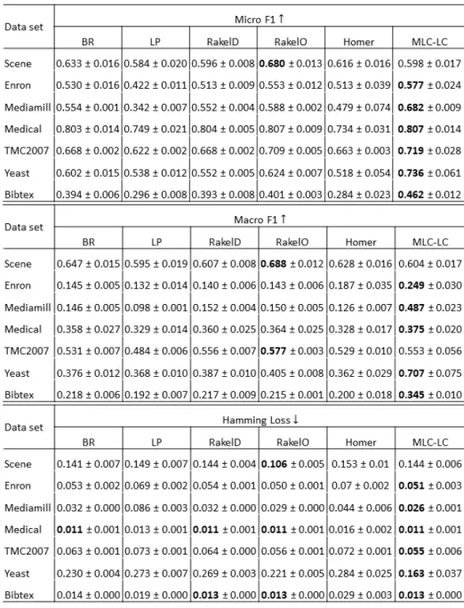
Figure 4.1presents the average and standard deviation of the micro-F1, macro-F1

and hamming loss score measure for all MLC method-dataset pairs, for random sampling whereas 4.2shows the same for stratified sampling. Overall,MLC–LCshows

Figure 4.1: micro-F1, macro-F1and hamming Loss scores for 66% random sampling

train-ing set. Experimental results (mean±std) on data.↑(↓) indicates the larger (smaller), the

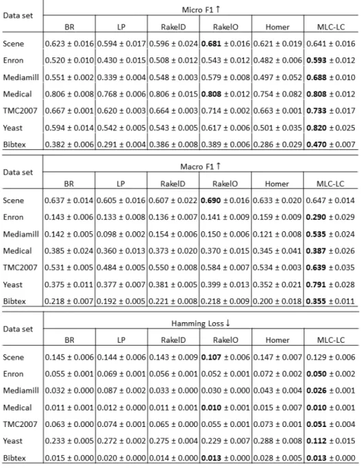
Figure 4.2: micro-F1, macro-F1 and hamming Loss scores for 66% stratified sampling

training set. Experimental results (mean±std) on data.↑(↓) indicates the larger (smaller),

Figure 4.3: Ranking of MLC methods according to their micro-F1, macro-F1and hamming

loss scores for 66% random sampling training set

comparatively best results for micro-F1and macro-F1scores over all the other MLC

algorithms except for Scene data set. It is same for hamming loss values, asMLC–LC shows the lowest loss for both random sampling and stratifies sampling results. For Scene data set, MLC-LC method performs almost same as BR method, since Scene data set is clustered into six singleton clusters byMLC–LCclustering approach. As can be seen from these tables, all the evaluation results for stratified sampling are higher than

random sampling due to the higher quality of training set selection.

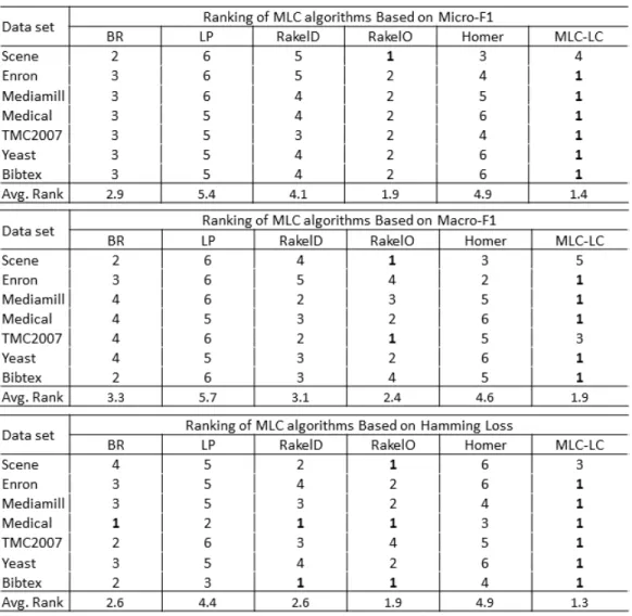
Figures 4.3and4.4show the ranking of different MLC algorithms on different data sets based on evaluation scores for random and stratified sampling respectively. The

Figure 4.4: Ranking of MLC algorithms Based on micro-F1, macro-F1and hamming Loss

score for stratified sampling

rows in the tables are the data sets and the columns list the MLC algorithms, except the last row which lists the average rank of each MLC algorithm. For an example, an entry in rowiand columnjin the first table in 4.3lists the rank of the micro-F1score on the data

setiof the micro-F1of the MLC algorithm corresponding toj. As can be seen from the

average rankrows of these two tables,MLC–LChas the best performance over all other MLC algorithms and RAkELo has the next best performance.

To explain further insights of MLC–LCperformances, sub-experiment was conducted on label level evaluation. Figure 4.5shows the label-wiseF1score for all the

Figure 4.5: F1 scores for Yeast data set with 66% random sampling training set and 34%

testing set

labels in Yeast data set, which shows significantly higher micro-F1and macro-F1

compare to the other MLC algorithms. The superior performance ofMLC–LCcan be clearly seen from this figure as partitioning method uses inMLC–LCenhances the predictive performances by categorizing labels by preserving the label dependencies.

Another additional feature introduced inMLC–LCis balancing column (a). It is a

common characteristic in most of the multi-label datasets that label per instance is low compared to all possible labels in the dataset (Label density). Hence, partitioning the label space into smaller parts introduces a large number of all zero LP label combinations within partitions. This leads to decrease predictive performances for some of the labels with positive bias also known as class imbalance problem.MLC–LCalgorithm considers about the biasness statistics of the labels within clusters in the training set and

determines whether or not to append balancing column into it. This is another reason for higher predictive performances of the proposed method.

4.2.2

Classification Accuracy with Different Training Set Sizes

This experiment is to illustrate how training set size effects on the predictive performance of MLC-LC compared to the other MLC methods. For this experiment different holdout partitions with 70%, 50%, and 30% of the datasets considered as the training and rest as the testing set. The holdout partitioning is done for both random and stratified as mentioned in the section IV(D). Multi-label classifiers were built using BR, LP, HOMER, RAkELd, RAkELo, andMLC–LCmethods. The results are evaluated using micro-F1, macro-F1and Hamming Loss matrices. Figure 4.6, Figure 4.7and

Figure 4.8show the results for 70%, 50%, and 30% training set and testing set selections respectively.

It can be seen thatMLC–LCmethod outperforms all the other MLC methods, even with small training set sizes such as 30%. At the same time, it is clear that RAkELo is the only MLC method which performs closer to theMLC–LCresults. Superior results of MLC-LC obviously hold as the training size increases despite of the diversity of the dataset it tested. We also ranked the relative performances (micro-F1, macro-F1and

hamming loss) of each MLC algorithm on each dataset for different training set sizes. According to the average ranking of the performances (given a rank 1, indicates the best performance for a given evaluation score and rank of 2 if it achieves the second highest score, etc),MLC–LCmethod shows smaller value as it consistently outperforms other MLC methods. Hence, in all case, both random and stratified sampling for the training set,MLC–LCperformed better compared to all the other MLC methods it was compared with.

4.2.3

Classification with Different Label Clustering Algorithms

This experiment compared the performance of anMLC–LCclassifier using the label clusters obtained fromC3_M with those obtained from two popular clustering methods –

Figure 4.6: micro-F1, macro-F1Scores and hamming loss values of Different MLC

Figure 4.7: micro-F1, macro-F1Scores and hamming loss values of Different MLC

Figure 4.8: micro-F1, macro-F1 scores and hamming loss values of Different MLC

these clustering methods lack a crucial aspect – estimating the number of clusters appropriate for a data set. However, this is a central feature of theC3_{M method. It}

automatically estimates the number of clusters appropriate for a given data set. The number of clusters play a crucial role in the overall performance since they determine the number of classifiers (LP and BR) as well their complexity.

For each data set, we estimated the number of clusters usingC3Mmethod by

de-constructing theC3M estimation component and coupling this with other clustering

approaches. The multi-label classifiers generated from these clusters were then compared in terms of accuracy. TheC3_{Mestimation component was combined with}

K-means(C3K) and hierarchical agglomerative(C3H) clustering methods to partition

the label set into the specified number of label clusters.

TheK-means clustering, given the number of clusters (K) and randomly chosenK

labels as centroids (or seeds), iteratively groups labels with the centroids based on a similarity (or a distance) metric. InC3K, the estimation component ofC3M provides

the parameter valueKand the required number of centroids are randomly chosen. We

executed theK-means algorithm for 10 iterations, each iteration with different

randomly chosen seeds and merged the label clusters obtained from the 10 iterations. We used the Euclidean distance metric to compute the clusters.

Hierarchical agglomerative clustering is a bottom-up clustering method where clusters have sub-clusters. For this clustering method, clustering starts with each single label as a separate cluster. Then for each successive iteration, it merges the closest pair of clusters by satisfying some similarity criteria, until all the data is in one cluster. This method provides three different approaches to manipulate the cluster sizes, namely single linkage, complete linkage, and average linkage.29_{We used the complete linkage}

method forC3Hbecause it defines the dissimilarity value between two clusters to be the

maximum dissimilarity value between any single data point in the first cluster and any single data point in the second cluster. Then, in each stage of the clustering process two

clusters with the smallest dissimilarity score among them are combined into one cluster. Clusters are repeatedly merged until the number of clusters matches those estimated by theC3_{M algorithm for the given data set. We employed the Euclidean distance to}

compute the dissimilarity scores.

Table4.2shows the statistics of label clusters obtained from the three different methods. This experiment was conducted using the Yeast, Medical, Enron, Mediamill, and tmc2007 data sets. The first column in the table lists the name of the data set, second, third, and fourth columns list the minimum and maximum size of a cluster obtained fromC3_{M,C3KandC3Hclustering methods respectively. The last three}

columns list the standard deviation in the cluster sizes obtained fromC3_M,C3Kand

C3Hclustering methods respectively.

As can be seen from the table, although the number of label clusters for each data set is held constant for the three cluster methods, the actual partitioning of label set into different clusters was different in different methods. If we observe the standard deviation of the cluster sizes (columns namedsdM, sdK, andsdH),C3Mhas the least

value for most data sets. This is because the clusters generated fromC3_{M contain either}

many singleton clusters or a small number of larger size clusters. TheC3_Malgorithm

does not attempt to balance the cluster sizes and groups labels completely based on cover-coefficient values and do not typically group unrelated labels into the same cluster. However, the deviation in cluster sizes among the three methods did not have a

significant impact on the classification accuracy as discussed below. Perhaps, this is because the labels grouped into the same cluster by the three different methods were largely similar.

Once the label clusters are constructed, the steps outlined in Section3.2were repeated and trained a BR or an LP classifier based on the size of a label cluster. We then performed holdout cross-validation with the random sample of 66% for training and rest for testing. Testing results are evaluated using micro-F1and macro-F1values, which are

Data M K H sdM sdK sdH Yeast 1,10 4,6 2,8 4.72 1.54 3.1 Medical 1,8 1,15 1,15 1.3 2.5 2.5 Enron 1,22 1,35 1,28 5.5 8.7 9.5 Mediamill 1,25 1,74 1,79 7.0 16.6 17.8 tmc2007 1,11 1,14 1,14 3.3 4.3 4.3

Table 4.2: Label Clustering using C3M, C3K, and C3H methods

displayed in Figure4.9. From this figure, it can be seen that the predictive performance of the three multi-label classifiers obtained from the three different cluster methods is approximately the same with respect to the micro-F1and macro-F1measures. The small

fluctuations in the micro and macro-F1scores are perhaps due to the small variations in

the set of labels grouped into the same cluster by the three different clustering methods. We also computed the Hamming loss of the three multi-label classifiers. We

observed that the Hamming loss was small at most 0.189 and as small as 0.009. The Hamming loss of the three multi-label classifiers was almost the same for the Enron, Mediamill, and the tmc2007 data sets. In case of the Yeast and the Medical data sets, the multi-label classifier obtained fromC3Hhad the smallest Hamming loss.

This experiment shows that the choice of clustering method may not affect the predictive performance of the multi-label classifier. However, estimating the

appropriate number of clusters for a data set usingC3_M can be a powerful tool that can

be combined with any clustering algorithm such as theK-means to obtain appropriate

partitioning of the data set. Although there are other methods for estimating the number of clusters such as thegap statistic30method for a given data set, the estimation method used byC3Manalyzes the data dependencies to compute the number of clusters, and

hence, possibly more accurate.

In case of sparse label sets, the implementation ofC3_{Mis typically more efficient}

since it exploits the sparsity in the data. Therefore, one can say that combining the number of clusters estimation fromC3_Mand then using any other clustering algorithm

Figure 4.9: (a) Micro-F1and (b) Macro-F1scores of theMLC–LCClassifiers Obtained from

Different Clustering Methods

to find clusters may not be more time-consuming. We are currently studying the cost of executingC3KandC3Hon large data sets.

In our experiments, we observed that the RAkELo method was performing either as well asMLC–LCor as the next best algorithm on most data sets and experimental

settings. This is not surprising as bothMLC–LCand RAkELo attempt to incorporate label correlations into the classification process. In RAkELo, overlapping subsets of labels are created so that label correlations get appropriate coverage and the voting system

ultimately chooses the appropriate label combination for a given instance during the testing phase. In contrast,MLC–LCcomputes the label clusters while preserving the label correlations and the prediction phase is a simple union of predicted labels from multiple LP/BR classifiers.

Chapter 5

CONCLUSIONS AND FUTURE WORK

The multi-label classification methodology which incorporates higher-order label correlations into learning called themulti-label classification with label clusters (MLC–LC) proposed in this study is a problem-transformation method. The label set is first partitioned into label clusters depending on how they co-occur in the data set. The training set is constructed from the original data set for each label cluster by including only the labels that occur in the label cluster for each training instance to train a classifier. Therefore, there are as many classifiers as the number of label clusters. Each classifier predicts a set of labels for each test instance. These labels are then unioned to generate the final set of labels.C3_M, a novel clustering algorithm, is used to generate

label clusters. Unique features ofC3_M include automatically estimating the appropriate

number of clusters for a given data set and automatically selecting the cluster seeds. Based on our experimental results, theMLC–LChas superior predictive performance over established MLC techniques such as RAkELd, RAkELo, HOMER, etc., on several diverse multi-label data sets. The superior predictive performance of theMLC–LCdoes not suffer even when the training set size is reduced to just 30% of the data set. The classification accuracy of theMLC–LCtechnique when the label clusters are generated is compared using well-known clustering techniques –K-means and complete linkage

HAC. The number of label clusters appropriate for each label set computed byC3_{M was}

provided to these algorithms as an input. It may be because of these reasons that the classification accuracies of the MLC classifiers constructed using label clusters from all three clustering methods were very similar.

In future, we plan to study how to incorporate the effect of feature vector similarity (or dissimilarities) into label correlations. Also, this study can be further improved to accommodate databases with missing labels. Missing labels is one of the major problems that reduces the performance of classification as for some instances are not assigned labels completely. AsC3_{M method is capable enough to extract label dependencies, it is}

possible to extend the current study to impute missing labels. Further, we planned to improve the performance of multi-label classification in data streams as another possible future direction since it requires updating the models incrementally. In stream data, it is challenging to maintain label dependencies as new labels may be added or removed as new instances are continuously Incorporated into the analysis.

References

[1] Eva Gibaja and Sebastian Ventura. A tutorial on multi-label learning. ACM Computing Surveys, 47, 04 2015.

[2] G. Tsoumakas, I. Katakis, and I. Vlahavas. Effective and Efficient Multilabel

Classification in Domains with Large Number of Labels. InProc. ECML/PKDD 2008 Workshop on Mining Multidimensional Data (MMD’08), page XX, 2008.

[3] B. Zhang, Y. Wang, and F. Chen. Multilabel image classification via high-order label correlation driven active learning.IEEE Transactions on Image Processing,

23(3):1430–1441, March 2014.

[4] Eyke HÃijllermeier, Johannes FÃijrnkranz, Weiwei Cheng, and Klaus Brinker. Label ranking by learning pairwise preferences.Artificial Intelligence, 172(16):1897 – 1916, 2008.

[5] Nadia Ghamrawi and Andrew McCallum. Collective multi-label classification. In Proceedings of the 14th ACM International Conference on Information and Knowledge Management, CIKM ’05, pages 195–200, New York, NY, USA, 2005. ACM.

[6] Johannes Fürnkranz, Eyke Hüllermeier, Eneldo Loza Mencía, and Klaus Brinker. Multilabel classification via calibrated label ranking. Mach. Learn., 73(2):133–153, November 2008.

[7] Grigorios Tsoumakas and Ioannis Vlahavas. Random k-Labelsets: An Ensemble Method for Multilabel Classification, pages 406–417. Springer Berlin Heidelberg, Berlin, Heidelberg, 2007.

[8] Fazli Can and Esen A. Ozkarahan. Concepts and effectiveness of the

cover-coefficient-based clustering methodology for text databases. ACM Trans. Database Syst., 15(4):483–517, December 1990.

[9] M. Zhang and Z. Zhou. A review on multi-label learning algorithms. Knowledge and Data Engineering, IEEE Transactions on, PP(99):1, 2013.

[10] C.X. Li. Exploiting Label Correlations for Multi-label Classification. University of California, San Diego, 2011.

[11] Grigorios Tsoumakas, Ioannis Katakis, and Ioannis Vlahavas. Random k-labelsets for multi-label classification.IEEE Transactions on Knowledge and Data Engineering, 99(1), 2010.

[12] Shan Wu, Shangfei Wang, and Qiang Ji. Capturing dependencies among labels and features for multiple emotion tagging of multimedia data. InAAAI, 2017.

[13] Shangfei Wang, Jun Wang, Zhaoyu Wang, and Qiang Ji. Enhancing multi-label classification by modeling dependencies among labels.Pattern Recognition, 47(10):3405 – 3413, 2014.

[14] Grigorios Tsoumakas and Ioannis Katakis. Multi-label classification: An overview. Int J Data Warehousing and Mining, 2007:1–13, 2007.

[15] Jesse Read. A pruned problem transformation method for multi-label classification. InIn: Proc. 2008 New Zealand Computer Science Research Student Conference (NZCSRS, pages 143–150, 2008.