HYSY
S
3.2
Hyprotech is the owner of, and have vested in them, the copyright and all other intellectual property rights of a similar nature relating to their software, which includes, but is not limited to, their computer programs, user manuals and all associated documentation, whether in printed or electronic form (the “Software”), which is supplied by us or our subsidiaries to our respective customers. No copying or reproduction of the Software shall be permitted without prior written consent of Aspen Technology,Inc., Ten Canal Park, Cambridge, MA 02141, U.S.A., save to the extent permitted by law.
Hyprotech reserves the right to make changes to this document or its associated computer program without obligation to notify any person or organization. Companies, names, and data used in examples herein are fictitious unless otherwise stated.
Hyprotech does not make any representations regarding the use, or the results of use, of the Software, in terms of correctness or otherwise. The entire risk as to the results and performance of the Software is assumed by the user.
HYSYS, HYSIM, HTFS, DISTIL, and HX-NET are registered trademarks of Hyprotech. PIPESYS is a trademark of Neotechnology Consultants.
Multiflash is a trademark of Infochem Computer Services Ltd, London, England.
PIPESIM2000 and PIPESIM are components of the PIPESIM Suite from Baker Jardine and Associates, London, England. All references to PIPESIM in this document refer to PIPESIM 2000.
Microsoft Windows 2000, Windows XP, Visual Basic, and Excel are registered trademarks of the Microsoft Corporation.
1 Black Oil ... 1-1
1.1 Black Oil Tutorial Introduction...1-2 1.2 Setting the Session Preferences ...1-4 1.3 Setting the Simulation Basis...1-9 1.4 Building the Simulation ...1-16
A Neotec Black Oil Methods ... 1-38
A.1 Neotec Black Oil Methods and Thermodynamics...1-39
B Black Oil Transition Methods ... 1-68 2 Multiflash for HYSYS Upstream... 2-1
2.1 Introduction...2-2 2.2 Multiflash Property Package...2-3
3 Lumper and Delumper ... 3-1
3.1 Lumper ...3-2 3.2 Delumper ...3-20 3.3 References ...3-36 4 PIPESIM Link ... 4-1 4.1 Introduction...4-2 4.2 Installation ...4-4 4.3 PIPESIM Link View...4-8 4.4 PIPESIM Link Tutorial ...4-22
5 PIPESIM NET ... 5-1
5.1 Introduction...5-2 5.2 PIPESIM NET...5-2
1 Black Oil
1.1 Black Oil Tutorial Introduction ...2
1.2 Setting the Session Preferences...4
1.2.1 Creating a New Unit Set...5
1.2.2 Setting Black Oil Stream Default Options...8
1.3 Setting the Simulation Basis ...9
1.3.1 Selecting Components ...9
1.3.2 Creating a Fluid Package ... 11
1.3.3 Entering the Simulation Environment ...13
1.4 Building the Simulation...16
1.4.1 Installing the Black Oil Feed Streams ...16
1.4.2 Installing Unit Operations ...26
1.1 Black Oil Tutorial Introduction
In HYSYS, Black Oil describes a class of phase behaviour and transport property models. Black oil correlations are typically used when a limited amount of oil and gas information is available in the system. Oil and gas fluid properties are calculated from correlations with their respective specific gravity (as well as a few other easily measured parameters). Black Oil is not typically used for systems that would be characterized as gas-condensate or dry gas, but rather for systems where the liquid phase is a non-volatile oil (and consequently there is no evolution of gas, except for that which is dissolved in the oil).In this Tutorial, two black oil streams at different conditions and compositions are passed through a mixer to blend into one black oil stream. The blended black oil stream is then fed to the Black Oil Translator where the blended black oil stream data is transitioned to a HYSYS material stream. A flowsheet for this process is shown below.
The following pages will guide you through building a HYSYS case for modeling this process. This example will illustrate the complete
construction of the simulation, from selecting the property package and components, to installing streams and unit operations, through to examining the final results. The tools available in the HYSYS interface will be used to illustrate the flexibility available to you.
The simulation will be built using these basic steps: 1. Create a unit set and set the Black Oil default options. 2. Select the components.
3. Add a Neotec Black Oil property package. 4. Create and specify the feed streams.
5. Install and define the unit operations prior to the translator. 6. Install and define the translator.
1.2 Setting the Session Preferences
1. To start a new simulation case, do one of the following:• From the File menu, select New and then Case. • Click the New Case icon.
The Simulation Basis Manager appears:
Next you will set your Session Preferences before building a case.
Figure 1.2
2. From the Tools menu, select Preferences. The Session Preferences view appears. You should be on the Options page of the Simulation
tab.
3. In the General Options group, ensure the Use Modal Property Views
checkbox is unchecked so that you can access multiple views at the same time.
1.2.1 Creating a New Unit Set
The first step in building the simulation case is choosing a unit set. Since HYSYS does not allow you to change any of the three default unit sets listed (i.e., EuroSI, Field, and SI), you will create a new unit set by cloning an existing one. For this example, a new unit set will be made based on the HYSYS Field set, which you will then customize.
To create a new unit set, do the following:
1. In the Session Preferences view, click the Variables tab. 2. Select the Units page if it is not already selected.
3. In the Available Unit Setsgroup, highlight Field to make it the active set.
4. Click the Clone button. A new unit set named NewUser appears. This unit set becomes the currently Available Unit Set.
5. In the Unit Set Name field, rename the new unit set as Black Oil. You can now change the units for any variable associated with this new unit set.
In the Display Units group, the current default unit for Std Gas Den is lb/ft3. In this example we will change the unit to SG_rel_to_air.
Figure 1.4
The default Preference file is named hysys.PRF. When you modify any of the preferences, you can save the changes in a new Preference file by clicking the Save Preference Set button. HYSYS prompts you to provide a name for the new Preference file, which you can load into any simulation case by clicking the Load Preference Set button.
6. To view the available units for Std Gas Den, click the drop-down arrow in the Std Gas Den cell.
7. Scroll through the list using either the scroll bar or the arrow keys, and select SG_rel_to_air.
8. Next change the Standard Density unit to SG 60/60 api. Your Black Oil unit set is now defined.
1.2.2 Setting Black Oil Stream Default Options
To set the Black Oil stream default options:
1. Click on the OilInput tab in the Session Preference view. 2. In the Session Preferences view, select the Black Oils page.
3. In the Black Oil Stream Options group, you can select the methods for calculating the viscosity, and displaying the water content for all
the black oil streams in your simulation. For now you will leave the settings as default.
4. Click the Close icon (in the top right corner) to close the Session Preferences view. You will now add the components and fluid package to the simulation.
Figure 1.6
1.3 Setting the Simulation Basis
The Simulation Basis Manager allows you to create, modify, and manipulate fluid packages in your simulation case. As a minimum, a Fluid Package contains the components and property method (for example, an Equation of State) HYSYS will use in its calculations for a particular flowsheet. Depending on what is required in a specific flowsheet, a Fluid Package may also contain other information such as reactions and interaction parameters. You will first define your fluid package by selecting the components in this simulation case.1.3.1 Selecting Components
HYSYS has an internal stipulation that at least one component must be added to a component list that is associated to a fluid package. To fulfil this requirement you must add a minimum of a single component even when the compositional data is not needed. For black oil streams, depending on the information available, you have the option to either specify the gas components compositions or the gas density to define the gas phase of the stream.
To add components to your simulation case:
1. Click on the Components tab in the Simulation Basis Manager. 2. Click the Add button. The Component List view is displayed.
In this tutorial, you will add the following components: C1, C2, C3, i-C4,
n-C4, i-C5, n-C5, and C6.
For more information on adding and viewing components, refer to
Chapter 1 - Components in the Simulation Basis.
3. Close the Component List View to return to the Simulation Basis Manager view.
Figure 1.7
If the Simulation Basis Manager is not visible, select the Home View icon from the tool bar.
1.3.2 Creating a Fluid Package
In this tutorial, since a Black Oil Translator is used in transitioning a Black Oil stream to a HYSYS compositional stream, two property packages are required in the simulation. You will first add the Neotec Black Oil property package and later in the tutorial after, you have installed the black oil translator, you will add the Peng-Robinson property package.
Adding the Neotec Black Oil Property Package
To add the Neotec Black Oil Property Package to your simulation: 1. From Simulation Basis Manager, click the Fluid Pkgs tab.2. Click the Add button in the Current Fluid Packages group. The Fluid Package Manager appears.
3. In the Component List Selection group, select Component List - 1
from the drop-down list.
4. From the list of available property packages in the Property Package Selection group, select Neotec Black Oil. The Neotec Black Oil selection view appears.
5. In the Basis Field, rename the newly added fluid package to Black Oil.
Figure 1.8
You can also filter the list of available property packages by clicking the
Miscellaneous Type radio button in the Property Package Filter group. From the filtered list you can select Neotec Black Oil.
The Advanced button allows you to return to the Fluid Package Manager view.
6. Click the Launch Neotec Black Oil button. The Neotec Black Oil Methods Manager appears.
The Neotec Black Oil Methods Manager displays the nine PVT behaviour and transport property procedures, and each of their calculation methods.
7. In this tutorial, you want to have the Watson K Factor calculated by the simulation. The default option for the Watson K Factor is set at Specify. Thus, you will change the option to Calculate from the Watson K Factor drop-down list, as shown below.
Figure 1.9
Figure 1.10
The User-Selected radio button is automatically activated when you select a Black Oil method that is not the default.
Refer to Appendix A - Neotec Black Oil Methods for more information on the black oil methods available and other terminology.
You can restore the default settings by clicking on the Black Oil Defaults radio button.
8. Click the Close button to close the Neotec Black Oil Methods Manager.
The Black Oil fluid package is now completely defined. If you click on the Fluid Pkgs tab in the Simulation Basis Manger you can see that the list of Current Fluid Packages now displays the Black Oil Fluid Package and shows the number of components (NC) and property package (PP). The newly created Black Oil Fluid Package is assigned by default to the main flowsheet. Now that the Simulation Basis is defined, you can install streams and operations in the Main Simulation environment. To leave the Basis environment and enter the Simulation environment, do one of the following:
• Click the Enter Simulation Environment button on the Simulation Basis Manager view.
• Click the Enter Simulation Environment icon on the tool bar.
1.3.3 Entering the Simulation Environment
When you enter the Simulation environment, the initial view that appears depends on your current Session Preferences setting for the Initial Build Home View. Three initial views are available:
1. PFD
2. Workbook
3. Summary
Enter Simulation Environment icon
Any or all of these can be displayed at any time; however, when you first enter the Simulation environment, only one appears. In this example, the initial Home View is the PFD (HYSYS default setting).
There are several things to note about the Main Simulation
environment. In the upper right corner, the Environment has changed from Basis to Case (Main). A number of new items are now available in the menu bar and tool bar, and the PFD and Object Palette are open on the Desktop. These latter two objects are described below.
Before proceeding any further, save your case. Do one of the following:
• Click the Save icon on the tool bar. • From the File menu, select Save. • Press CTRLS.
If this is the first time you have saved your case, the Save Simulation Case As view appears.
Objects Description
PFD The PFD is a graphical representation of the flowsheet topology for a simulation case. The PFD view shows operations and streams and the connections between the objects. You can also attach information tables or annotations to the PFD. By default, the view has a single tab. If required, you can add additional PFD pages to the view to focus in on the different areas of interest.
Object Palette A floating palette of buttons that can be used to add streams and unit operations.
Figure 1.12
You can toggle the palette open or closed by pressing F4, or by selecting the Open/Close Object Palette command from the Flowsheet menu.
By default, the File Path is the Cases sub-directory in your HYSYS directory. To save your case, do the following:
1. In the File Name cell, type a name for the case, for example
BlackOil. You do not have to enter the .hsc extension; HYSYS automatically adds it for you.
2. Once you have entered a file name, press the ENTER key or click the
Save button. HYSYS saves the case under the name you have given it when you save in the future. The Save As view will not appear again unless you choose to give it a new name using the Save As
command. If you enter a name that already exists in the current directory, HYSYS will ask you for confirmation before over-writing the existing file.
1.4 Building the Simulation
1.4.1 Installing the Black Oil Feed Streams
In this tutorial, you will install two black oil feed streams. To add the first black oil stream to your simulation do one of the following:
1. From the Flowsheet menu, select Add Stream. The Black Oil Stream property view appears.
OR
1. From the Flowsheet menu, select Palette. The Object Palette appears.
2. Double-click on the Material Stream icon. The Black Oil Stream property view appears.
When you choose to open an existing case by clicking the
Open Case icon , or by
selecting Open Case from the File menu, a view similar to the one shown in Figure 1.12 appears. The File Filter drop-down list will then allow you to retrieve backup (*.bk*) and HYSIM (*.sim) files in addition to standard HYSYS (*.hsc) files.
You can also add a new material stream by pressing the F11 hot key.
You can open the Object Palette by clicking the Object Palette icon.
Object Palette icon
HYSYS displays three different phases in a black oil stream. The three phases are:
• Gas • Oil • Water
The first column is the overall stream properties column. You can view and edit the Gas, Oil, and Water phase properties by expanding the width of the default Black Oil stream property view (Figure 1.13). You can also use the horizontal scroll bar to view all the phase properties.
The expanded stream property view is shown below.
3. You can rename the stream to Feed1 by typing the new stream name directly in the Stream Name cell of the Overall column (first column).
Figure 1.14
You can only rename the overall column, and that name will be
displayed on the PFD as the name for that black oil stream. You cannot change the phase name for the stream.
Next you will define the gas composition in Feed 1.
1. On the Worksheet tab, click on the Gas Composition page to begin the compositional input for the stream.
2. Check the Activate Gas Composition checkbox to activate the Gas Composition table.
The Activate Gas Composition checkbox allows you to specify the compositions for each base component you selected in the Simulation Basis manager. After you have defined the gas composition for the black oil stream, HYSYS will automatically calculate the specific gravity for the gas phase. If gas composition information is not available, you can provide only the specific gas gravity on the Conditions page to define the black oil stream.
3. Click on the Edit button. The Input Composition for Stream view appears. By default, you can only specify the stream compositions in mole fraction.
4. Enter the following composition for each component:
5. Click the OK button, and HYSYS accepts the composition.
Figure 1.16
Component Mole Fraction
Methane 0.3333 Ethane 0.2667 Propane 0.1333 i-Butane 0.2000 n-Butane 0.0677 i-Pentane 0.0000 n-Pentane 0.0000 n-Hexane 0.0000
Once you have specified the composition for C1 to n-C4, you can click the Normalize button, and HYSYS will ensure that the Total is equal 1.0, while also specifying any <empty> compositions (in this case, i-C5 to C6) as zero.
6. Click on the Conditions page on the Worksheet tab.
Next you will define the conditions for Feed 1.
1. In the overall column (first column), specify the following conditions:
HYSYS should automatically assign the same temperature and pressure to the Gas, Oil, and Water phases.
2. Specify the Specific Gravity for the Oil phase and Water phase to
0.847 SG_60/60 api and 1.002 SG_60/60 api, respectively. Next you will specify the bulk properties for Feed 1.
1. In the Bulk Properties group, specify a Gas Oil Ratio of 1684 SCF/ bbl, and Water Cut of 15%.
Figure 1.17
In this cell... Enter...
Temperature (°C) 50
Pressure (kPa) 101.3
Volumetric Flow (barrel/day) 4500
The Gas Oil Ratio is the ratio of the gas volumetric flow to oil volumetric flow at stock tank conditions. The Gas Oil Ratio will be automatically calculated if the volumetric flows of the gas, oil, and water phases are known. In this tutorial, the volumetric flowrates for the three phases are calculated by the Gas Oil Ratio and Water Cut.
The water content in the Black Oil stream can be expressed in two ways:
• Water Cut. The water cut is expressed as a percentage.
where: Vwater = volume of water Voil = volume of oil
• WOR. A ratio of volume of water to the volume of oil.
You can select your water content input preference from the drop-down list.
Next you will specify a method for calculating the dead oil viscosity. 1. Click on the Viscosity Mtd button. The Black Oil Viscosity Method
Selection view appears.
(1.1)
(1.2)
Figure 1.19
Water Cut Vwater
Voil+Vwater ---= WOR Vwater Voil ---= Viscosity Mtd button
Displays the current selection of the Dead Oil Viscosity Equation. You can change this equation in the Neotec Black Oil Methods Manager. Refer to Dead Oil Viscosity Equation in Appendix A.1 - Neotec Black Oil Methods and Thermodynamics for more information.
You can select the calculation methods from the Method Options drop-down list. Neotec recommends the user to enter two or more viscosity data points. In the event that only one data point is known, this is also an improvement over relying on a generalized viscosity prediction. 2. Click on the Method Options drop-down list and select Twu. 3. Close the Black Oil Viscosity Method Selection view.
Now Feed 1 is fully defined.
The Surface Tension and Watson K are automatically calculated by HYSYS as specified in the Neotec Black Oil Methods Manager. You can view the property correlations for each phase by clicking on the Properties page where you can add and delete correlations as desired.
Next create a second black oil feed stream, Feed 2 and define it with the following data:
In these cells... Enter...
Conditions
Temperature (°F), Overall 149 Pressure (psia), Overall 29.01 Volumetric Flow (barrel/day), Overall 6800 Specific Gravity (SG_60/60 api) Oil: 0.8487
Water: 1.002
Gas Oil Ratio 1404 SCF/bbl
Water Cut 1.5
Viscosity Method Options Beggs and Robinson Gas Composition
Methane 1.0
1.4.2 Installing Unit Operations
Now that the two black oil feed streams are fully defined, the next step is to install the necessary unit operations for the transitioning process.
Installing the Valve
The first operation that will be installed is a Valve, used to decrease the pressure of Feed 1 before it is blended with Feed 2.
1. Double-click on the Valve icon in the Object Palette. The Valve property view appears.
2. On the Connections page, open the Inletdrop-down list by clicking on .
3. Select Feed 1 from the list.
4. Move to the Outlet field by clicking on it. Type ValveOut in the Outlet cell and press ENTER.
The status indicator displays ‘Unknown Delta P’. To specify a pressure drop for the Valve:
1. Click on the Parameters page. 2. Specify 5 kPa in the Delta P field.
Now the status indicator has changed to green OK, showing that the valve operation and attached streams are completely calculated.
Figure 1.23
The following unit operations can support black oil streams:
• Valve • Mixer • Pump • Recycle • Separator • Pipe Segment • Heat Exchanger • Expander • Compressor • Heater • Cooler Valve icon
Alternatively, you can make the connections by typing the exact stream name in the cell, then pressing ENTER.
Installing the Mixer
The second operation that will be installed is a Mixer, used to blend the two black oil feed streams.
To install the Mixer:
1. Double-click on the Mixer icon in the Object Palette. The Mixer property view appears.
2. Click the <<Stream>> cell to ensure the Inlets table is active. The status bar at the bottom of the view shows that the operation requires a feed stream.
Figure 1.24
3. Open the <<Stream>> drop-down list of feeds by clicking on or by pressing the F2 key and then the Down arrow key.
4. Select ValveOut from the list. The stream is transferred to the list of Inlets, and <<Stream>> is automatically moved down to a new empty cell.
5. Repeat steps 3-4 to connect the other stream, Feed 2.
The status indicator now displays ‘Requires a product stream’. Next you will assign a product stream.
6. Move to the Outlet field by clicking on it, or by pressing TAB.
Figure 1.25
Alternatively, you can make the connections by typing the exact stream name in the cell, then pressing ENTER.
7. Type MixerOut in the cell, then press ENTER. The status indicator now displays a green OK, indicating that the operation and attached streams are completely calculated.
8. Click the Parameters page.
9. In the Automatic Pressure Assignment group, leave the default setting at Set Outlet to Lowest Inlet.
Figure 1.26
Figure 1.27
HYSYS recognizes that there is no existing stream named MixerOut, so it will create the new stream with this name.
HYSYS has calculated the outlet stream by combining the two inlets and flashing the mixture at the lowest pressure of the inlet streams. In this case, ValveOut has a pressure of 96.3 kPa and Feed 2 has a pressure of 200 kPa. Thus, the outlet from the Mixer has a pressure of 96.3 kPa (the lowest pressure between the two inlets).
Refer to Appendix A - Neotec Black Oil Methods, for more information on the specific gravity and viscosity of heavy oil/condensate blends.
Installing the Black Oil Translator
Next you will install a Black Oil Translator to transfer the black oil stream data into a compositional stream so that you can analyze the properties of the blended black oil stream from the Mixer. The Black Oil Translator is implemented in HYSYS using the Stream Cutter operation and a custom Black Oil Transition. The Black Oil Translator interacts with an existing Stream Cutter unit operation to convert the Black Oil stream into a compositional material stream.
Adding the Black Oil Translator
There are two ways that you can add the Black Oil Translator to your simulation:
1. From the Flowsheet menu, select Add Operation. The UnitOps view appears.
2. In the Categories group, select the All Unit Ops radio button. 3. From the Available Unit Operation lists, select Black Oil Translator. 4. Click Add. The Black Oil Translator property view appears.
OR
The Worksheet tab is not supported when the unit operation is used in Black Oil mode.
You can also open the UnitOps view by pressing the F12 hot key.
1. From the Object Palette, click on the Upstream Ops icon. The Upstream Ops Palette appears.
2. Double-click the Black Oil Translator icon. The Black Oil Translator property view appears.
In certain situations, the Black Oil Translator will automatically be added to the flowsheet. This occurs when the stream connections are made to operations that have streams with different fluid packages connected or the operation itself is set to use a different fluid package. The Stream Cutter dictates the rules for when the Black Oil Translator is automatically added.
To delete the Black Oil Translator operation, click the Delete button. HYSYS will ask you to confirm the deletion.
To ignore the Black Oil Translator operation during calculations, activate the Ignored checkbox. HYSYS completely disregards the
Figure 1.28
Figure 1.29
Upstream Ops icon
Black Oil Translator icon
You can also delete a Black Oil Translator by clicking on the Black Oil Translator icon on the PFD and pressing the DELETE key.
Defining the Black Oil Translator
To complete the Connections page:
1. Open the Inlet drop-down list by clicking on or by pressing the
F2 key and then the Down arrow key. 2. Select MixerOut as the inlet.
3. Move to the Outlet field by clicking on it.
4. Type Outlet in the cell, and press ENTER. HYSYS will automatically
creates a stream with the name you have supplied.
Next you will select the transition method: 1. Click on the Transitions tab.
2. Select the Transitions page. The transition table should contain the Black Oil Transition as shown in the figure below.
3. Click on the View button. The Black Oil Transition property view appears.
4. In the Black Oil Transition Method group, select the Three Phase
radio button.
5. The composition of MixerOut is copied to the composition table as shown in Figure 1.32. Leave the composition as default. Close the
Figure 1.31
Figure 1.32
If the transition table does not contain the Black Oil Transition, click the Add button to add the black oil transition. The Select Transition view appears. From the Select Transition, select the black oil transition you want to add. Refer to Adding the Black Oil Translator for more information.
Refer to Appendix B - Black Oil Transition Methods for more information on the Simple and Three Phase transition method.
The status indicator still displays ‘Not Solved’. To solve the Black Oil Translator, the outlet to the black oil transition method must be a non-black oil stream. Thus, you will need to add a new fluid package and assign it to the outlet stream.
To add a new fluid package:
1. Click on the Enter Basis Environment icon in the tool bar. The Simulation Basis Manager appears.
2. Click on the Fluid Pkgs tab. 3. Click Add.
4. Select Peng-Robinson from the property package list in the Property Package Selection group.
5. In the Name field, rename the fluid package to PR as shown below.
6. Close the Fluid Package view.
7. Click on the Return to Simulation Environment button in Simulation Basis Manger.
Figure 1.33
Enter Basis Environment icon
Return to Simulation Environment button
To assign the Peng-Robinson property package to Outlet:
1. Double-click on the Outlet stream. The Outlet stream property view appears.
2. Click on the Conditions page and move to the Fluid Package cell by clicking on it.
3. Open the Fluid Package drop-down list of fluid packages by clicking on .
4. Select PR from the list.
Once you selected PR as the fluid package, the Outlet stream property view is automatically changed to a HYSYS compositional stream. At the same time, the Black Oil Translator starts transitioning the black oil data to the Outlet stream. The solving status is indicated in the Object Status Window. As the Black Oil Translator is solving, a list of hypocomponents are generated in the Outlet stream to characterize a black oil stream from a compositional stream perspective. You can view each hypocomponent created in the Trace Window as the Black Oil Translator is solving.
1.4.3 Results
When the solving is completed, the status indicator for the Outlet stream and Black Oil Translator should be changed to a green OK, showing that both operations are completely defined.
1. In the Outlet stream property view, click on the Compositions page on the Worksheet tab.
2. In the component composition list, you can view the composition for all the hypocomponents created as well as the composition for C1 to C6.
3. Close the Outlet stream property view.
4. Double-click on the CUT-100 operation on the PFD. The black oil translator property view appears.
5. Click on the Worksheet tab.
Figure 1.35
On the Conditions page, the Compositional stream properties and conditions for the black oil stream MixerOut are displayed in the Outlet column. Now you can examine and review the results for the MixerOut stream as a compositional stream.
Figure 1.36
A Neotec Black Oil Methods
A.1 Neotec Black Oil Methods and Thermodynamics...39
A.1.1 Terminology...40 A.1.2 PVT Behaviour and Transport Property Procedures...55
A.1 Neotec Black Oil Methods and
Thermodynamics
You can select the desired black oil methods in the Neotec Black Oil Methods Manager.
Several black oil PVT calculation methods exist, each based on data from a relatively specific producing area of the world.
Correlations Data
Standing (1947) Correlation for Rs and Bo
Based on 22 California crude oil-gas systems. Lasater (1958) Correlation for Rs Developed using 158 data from 137 crude-oils from Canada, Western and mid-continent USA, and South America.
Vasquez and Beggs (1977) Correlations for Rs and Bo
Based on 6004 data. Developed using data from Mid-West and California crudes. Glaso (1980) Correlations for Rs
and Bo
For volatile and non-volatile oils. Developed using data from North Sea crudes. Al-Marhoun (1985, 1988, 1992)
Correlations for Rs and Bo
Based on data from Saudi crude oils and Middle East reservoirs.
Abdul-Majeed and Salman (1988) Correlation for Bo
Based on 420 data points from 119 crude oil-gas systems, primarily from Middle East reservoirs.
Dokla and Osman (1992) Correlations for Rs and Bo
Based on 51 bottomhole samples taken from UAE reservoirs.
Petrosky and Farshad (1993) Correlations for Rs and Bo
Based on 81 oil samples from reservoirs in the Gulf of Mexico.
A.1.1 Terminology
Before we discuss the PVT behaviour and transport property procedures, you should be familiar with the following terms:
• Stock Tank Conditions • Produced Gas Oil Ratio • Solution Gas Oil Ratio
• Viscosity of Heavy Oil/Condensate Blends • Specific Enthalpies for Gases and Liquids • Oil-Water Emulsions
Stock Tank Conditions
Stock tank conditions are the basic reference conditions at which the properties of different hydrocarbon systems can be compared on a consistent basis. The stock tank conditions are defined as 14.70 psia (101.325 kPa) and 60 °F (15°C).
Produced Gas Oil Ratio
The produced gas oil ratio is the total amount of gas that is produced from the reservoir with one stock tank volume of oil. Typical units are scf/stb or m3 at s.c./m3 at s.c.
Solution Gas Oil Ratio
The solution gas/oil ratio is the amount of gas that saturates in the oil at a given pressure and temperature. Typical units are scf/stb or m3at s.c./ m3 at s.c.
Above the bubble point pressure, for a given temperature, the solution gas/oil ratio is equal to the produced gas oil ratio. For stock tank oil (i.e., oil at stock tank conditions) the solution gas oil ratio is considered to be zero.
Viscosity of Heavy Oil/Condensate Blends
A common relationship for estimating the viscosity of a mixture of two hydrocarbon liquids is as follows:
where: µm= viscosity of the blended stream
µA = viscosity of liquid A
µB = viscosity of liquid B
CA= volume fraction of liquid A in the blended stream
For cases where , it is recommended by Shu (1984) that another correlation should be used to calculate the viscosity of the mixture assuming that liquid A is the heavier and more viscous fluid than liquid B.
where:
SA = specific gravity of liquid A SB = specific gravity of liquid B
(1.3) (1.4) (1.5) (1.6) µm µA CA µB 1–CA ( ) × = µA µB --->20 µm µA XA µB 1–XA ( ) × = XA αCA αCA+CB ---= α 17.04 S( A–SB) 0.5237 SA3.2745SB1.6316 Ln µA µB --- ---=
Data from two different crude oil/condensate blends have been used to compare the results predicted by Equation (1.3) and Equation (1.4)
through Equation (1.6). The following table contains the available data for the two oils and the condensate liquid.
To simplify viscosity calculations at intermediate temperatures, the data given in the above table for each liquid were fitted to the following form:
where: T = temperature, °C a, b = fitted constants
The resulting values of a and b are given in the following table.
In all cases, the fit is very accurate (maximum error is about 3.6%) and the use of Equation (1.7) introduces minimal error into the comparison.
Liquid API Gravity Specific Gravity Viscosity (mPa.s) 5°C 10°C 20°C Oil A 14.3 0.970 12840 7400 2736 Oil B 14.3 0.964 3725 2350 1000 Condensate 82.1 0.662 0.42 0.385 -(1.7) Liquid a b Oil A 849.0 3.07 Oil B 370.0 2.62 Condensate 0.28 0.44 µ a 100 1.8 T⋅ +32 --- ⋅ b =
Measured data were available at three temperatures (0°C, 5°C, and 10°C) for each of the crude oils with three blending ratios (90%, 80%, and 70% crude oil). Mixture viscosities calculated by Equation (1.3) and
Equation (1.4) are compared with these data in the following table.
From the table it is clear that the results calculated using Equation (1.3)
are not acceptable and would lead to gross errors calculated pressure losses. As for Equation (1.4), it gives excellent results for the blends involving Oil A. While the errors associated with Oil B blends are significantly larger, they are not unreasonable.
Oil Temp (°C) Blend (% crude) µmeas (mPa.s) Equation 1.3 Equation 1.4 µcalc (mPa.s) error (%) µcalc (mPa.s) error (%) A 0 90 2220 9348 321.1 2392 7.8 A 0 80 382 3111 714.4 370 -3.1 A 0 70 89 1035 1062.9 86 -3.4 A 5 90 1464 4661 218.4 1442 -1.5 A 5 80 272 1656 508.2 260 -4.4 A 5 70 71 588 728.2 66 -7.0 A 10 90 976 2670 173.6 953 -2.4 A 10 80 198 999 404.6 194 -2.0 A 10 70 56 374 567.9 53 -5.4 B 0 90 744 2774 272.9 989 32.9 B 0 80 147 1056 618.4 205 39.5 B 0 70 45 402 793.3 58 28.9 B 5 90 516 1531 196.7 629 21.9 B 5 80 112 615 449.1 148 32.1 B 5 70 37 247 567.6 45 21.6 B 10 90 396 951 140.2 436 10.1 B 10 80 87 399 358.6 113 29.9 B 10 70 29 168 479.3 37 27.6
Equation (1.5) can be further modified to improve its accuracy by introducing a proprietary calibration factor.
The results obtained from the modified Shu correlation show that the calibration procedure has yielded a significant improvement in accuracy. This also applies to data at 0°C, which were not used in the determination of the calibration since no measured viscosity values for either Oil B or the condensate were available at that temperature. It has been demonstrated that the correlation of Shu (1984) is much superior to the simple blending relationship expressed by Equation (1.3), and it is capable of giving acceptable accuracy for most pipeline pressure drop calculations.
Specific Enthalpies for Gases and Liquids
The temperature profiles are calculated by simultaneously solving the mechanical and total energy balance equations. The latter includes a term that is directly related to changes in the total enthalpy of the fluid(s). This means that all Joule-Thompson expansion cooling effects for gases, and frictional heating effects for liquids would be taken into account implicitly. It is not necessary, for example, to impose the approximations inherent in specifying a constant average value of a Joule-Thompson coefficient. it is, however, necessary to be able to compute the specific enthalpy of any gas or liquid phase, at any pressure and temperature, as accurately as possible. The following sections describe the procedures for computing this important thermodynamic parameter for various fluid systems.
Oil Temp (°C) Blend (% crude) µmeas (mPa.s) Equation 1.4 µcalc (mPa.s) error (%) B 0 90 744 817 9.8 B 0 80 147 157 6.8 B 0 70 45 43 -4.4 B 5 90 516 529 2.5 B 5 80 112 115 2.7 B 5 70 37 34 -8.1 B 10 90 396 371 -6.3 B 10 80 87 90 3.4 B 10 70 29 28 -3.4
In pipelines and wells the Joule-Thompson effect is typically exhibited as a large decrease in temperature as a gas expands across a restriction. According to the relationships between the temperature, pressure, and latent energy of the fluid, the fluid typically cools when it expands, and warms when compressed.
Undefined Gases
For undefined single phase gases, where only the gravity is known, the specific enthalpy is determined by assuming the gas to be a binary mixture of the first two normal hydrocarbon gases whose gravities span that of the unknown gas. The mole fractions are selected such that the gravity of the binary mixture is identical to that of the unknown gas of interest.
For example, a natural gas having a gravity of 0.688 would be
characterized as a binary mixture consisting of 72.3 mole % methane (gravity = 0.5539) and 27.7 mole % ethane (gravity = 1.0382) since (0.723)(0.5539) + (0.277)(1.0382) = 0.688. The enthalpy of the binary mixture, calculated as described above for compositional systems, is then taken as the enthalpy of the gas of interest. This is in fact the same procedure that has been used to create the generalized specific enthalpy charts that appear in the GPSA Engineering Data Book (1987).
The specific enthalpy has been evaluated as described above for a number of specified gas gravities over a relatively wide range of pressures and temperatures. The enthalpy of the unknown gas is obtained at any given pressure and temperature by interpolation within the resulting matrix of values.
Undefined Liquids
Undefined hydrocarbon liquids are characterized only by a specific or API gravity, and possibly also the Watson K factor. They are also referred to as “black oils”, and the specific enthalpy is computed using the specific heat capacity calculated using the correlation of Watson and Nelson (1933):
where: Cp = specific heat capacity of the oil, btu/lb°F T = temperature, °F
(1.8) Cp = A1×[A2+(A3T)]
The three coefficients have the following equations:
where: K = Watson K factor = So = specific gravity of the oil
The specific enthalpy at any temperature T, relative to some reference temperature To, is given by the following equation:
The specific enthalpy computed using Equation (1.10) is independent of pressure. For real liquids, the effect of pressure is relatively small compared to the temperature effect, but it may become significant when the pressure gradient is large due to flow rate rather than elevation effects.
Large pressure gradients tend to occur with high viscosity oils. At higher flow rates, frictional heating effects can become significant, and the heating tends to reduce the oil viscosity, which in turn, affects the pressure gradient. Unfortunately, this complex interaction cannot be predicted mathematically using specific enthalpy values that are independent of pressure. The net result is that the predicted pressure gradient will be higher than should actually be expected.
(1.9) (1.10) A1 = 0.055K+0.35 A2 = 0.6811–0.308γo A3 = 0.000815–0.000306γo TB1 3⁄ So ---H Cp( )T dT To T
∫
=For fully compositional systems, the calculated specific enthalpy of a liquid phase does include the effect of pressure. A series of calculations have been performed using the Peng-Robinson (1976) equation of state for a variety of hydrocarbon liquids, ranging from relatively light condensate liquids to relatively heavy crude oils. In each case, specific enthalpy was calculated over a wide range of pressures at a low,
moderate, and high temperature. In the case of the condensate liquids, specific compositional analyses were used. For the heavier crude oils, the composition consisted of a number of pseudo-components, based on published boiling point assay data, as generated by Neotec’s technical utility module HYPOS. In all cases, the effect of pressure was found to be constant and is well represented by the following relation:
where: HP,T = specific enthalpy at the specific pressure and temperature, btu/ lb-°F
HPo,T = specific enthalpy computed with Equation (1.10)
P = pressure, psia
Figure 1.38, Figure 1.39, and Figure 1.40 show the comparison between specific enthalpies calculated using the Peng Robinson equation of state and those computed using Equation (1.11) for 16.5, 31.9, and 40.5° API oils, respectively. For comparison purposes, HPo,Twas taken to be the
value computed by the Peng Robinson equations of state at 15 psia.
(1.11) HP T, H
Po,T+0.0038×(P–15)
Effect of Pressure on Specific Enthalpy for a 16.5° API Oil
Effect of Pressure on Specific Enthalpy for a 40.5° API Oil
Figure 1.38
Effect of Pressure on Specific Enthalpy for a 31.9° API Oil
The effect of pressure is included in all specific enthalpy calculations, and therefore, in all temperature profile calculations, in a way that closely approximates similar calculations for fully compositional systems.
Oil-Water Emulsions
The rheological behaviour of emulsions may be non-Newtonian and is often very complex. Generalized methods for predicting transport properties are limited because of the wide variation in observed properties for apparently similar fluids. It is usually the case with non-Newtonian fluids that some laboratory data or other experimental observations are required to provide a basis for selecting or tuning transport property prediction methods.
Neotec assumed that an emulsion behaves as a pseudo-homogeneous mixture of hydrocarbon liquid and water and may thus be treated as if it were a single liquid phase with appropriately defined transport
properties.
The volumetric flow rate of this assumed phase is the sum of the oil and water volumetric flow rates,
where: Qe = volumetric flow rate of emulsion, ft3/sec or m3/sec Qo = volumetric flow rate of oil, ft3/sec or m3/sec Qw = volumetric flow rate of water, ft3/sec or m3/sec
The water volume fraction in the emulsion, Cw, is thus given by,
Since the emulsion is assumed to be a pseudo-homogeneous mixture, the density is given by,
where: ρe = density of the emulsion, lb/ft3 or kg/m3
ρw = density of the water at flowing conditions, lb/ft3 or kg/m3
ρo = density of the oil at flowing conditions, lb/ft3 or kg/m3
The effective viscosity of an emulsion depends on the properties of the oil, the properties of the water, and the relative amounts of each phase. For a water-in-oil emulsion (i.e. oil is the continuous phase), the effective viscosity of the emulsion can be much higher than that of the pure oil.
A commonly used relationship for estimating the viscosity of a water-in-oil emulsion is,
where: µe = viscosity of the emulsion, cP or mPa.s
µo = viscosity of the oil, cP or mPa.s
Fe = emulsion viscosity factor
(1.12) (1.13) (1.14) (1.15) Qe = Qo+Qw Cw Qw Qo+Qw ---= ρe = ρwCw+ρo(1–Cw) µe = Feµo
The factor Fe is usually considered to be a function of the water fraction Cw and the best known procedure for estimating Fe is the graphical correlation of Woelflin (1942).
More recently, Smith and Arnold (see Bradley, 1987) recommended the use of the following simple quadratic equation,
The emulsion viscosity factors based on Woelflin’s ‘medium’ emulsion curve (he also presented curves for ‘loose’ and ‘tight’ emulsions) are compared in Figure 1.41 with those calculated using Equation (1.16). The two relationships are virtually identical for Cw < 0.4, but diverge rapidly at higher values of Cw.
With increasing water fraction, the system will gradually behave more like water than oil. The water fraction at which the system changes from a water-in-oil emulsion to an oil-in-water emulsion is called the
inversion point. The transition to an oil-in-water emulsion is generally very abrupt and characterized by a marked decrease in the effective viscosity. The actual inversion point must usually be determined experimentally for a given system as there is no reliable way to predict it. In many cases however, it is observed to occur in mixtures consisting of
(1.16)
Figure 1.41
Guth and Simha (1936) proposed a similar correlation as Smith and Arnold (Equation (1.16)),
where: Fe = emulsion viscosity multiplier for the continuous phase viscosity Cd = volume fraction of the dispersed phase
If Cwi is defined as the water fraction at the inversion point, then for Cw < Cwi, the emulsion viscosity is given by Equation (1.15), with Fe defined by Equation (1.16). However, for Cw > Cwi, the emulsion viscosity should be computed using the following expression,
where: µw = viscosity of the water phase, cP or mPa.s Fe = 1.0 + 2.5(1-Cw)+14.1(1-Cw)2
As shown in Equation (1.17), while the constant and the first order term on the right can be shown to have a theoretical basis, the squared term represents a purely empirical modification. It seems reasonable therefore to view the coefficient of the squared term (i.e., 14.1) as an adjustable parameter in cases where actual data are available.
(1.17)
(1.18) Fe = 1.0+2.5Cd+14.1Cd2
To illustrate the predicted effect of the inversion point, Figure 1.42
shows a case in which Cwi = 0.65. Also the corresponding curves for several different values of the coefficient of the squared term are compared.
The large decrease in the predicted value of the emulsion viscosity is evident. The effect on the emulsion viscosity can be seen in Figure 1.43, since, above the inversion point, the factor is used to multiply the water viscosity, which is typically significantly lower than the oil viscosity.
Limited experience to date in performing pressure loss calculations for emulsions suggests that the Woelflin correlation over-estimates the viscosity at higher water fractions. It is thus recommended that one use the Guth and Simha equation unless available data for a particular case suggest otherwise.
A.1.2 PVT Behaviour and Transport Property
Procedures
There are nine PVT behaviour and transport property procedures available in the Neotec Black Oil Methods Manger:
• Solution GOR • Oil FVF
• Undersaturated Oil FVF • Gas Viscosity
• Live Oil Viscosity
• Undersaturated Oil Viscosity • Dead Oil Viscosity Equation • Watson K Factor
• Surface Tension
Solution GOR
The solution gas oil ratio, Rs, is the amount of gas that is assumed to be dissolved in the oil at a given pressure and temperature. Typical units are scf/stb or m3 at s.c./m3 at s.c.
Above the bubble point pressure, for a given temperature, the solution gas oil ratio is equal to the Produced Gas Oil Ratio. For the oil at Stock Tank Conditions, the solution gas oil ratio is considered to be zero. You can select one of the following methods to calculate the solution GOR:
• Standing. • Vasquez Beggs. • Lasater.
• Glaso (Non Volatile Oils) • Glaso (Volatile Oils) • Al Marhoun (1985)
• Al Marhoun (Middle East Oils) • Petrosky and Farshad
• Dolka and Osman
Oil FVF
The Oil Formation Volume Factor is the ratio of the liquid volume at stock tank conditions to that at reservoir conditions.
The formation volume factor (FVF, Bo) for a hydrocarbon liquid is the volume of one stock tank volume of that liquid plus its dissolved gas (if any), at a given pressure and temperature, relative to the volume of that liquid at stock tank conditions. Typical units are bbl/stb or m3/m3 at s.c. You can select one of the following methods to calculate the Oil FVF:
• Standing • Vasquez Beggs • Glaso
• Al Marhoun (1985),
• Al Marhoun (Middle East OIls) • Al Marhoun (1992)
• Abdul-Majeed and Salman • Petrosky and Farshad • Dolka and Osman
Undersaturated Oil FVF
In HYSYS, the default calculation method is Vasquez Beggs. You can choose other calculation methods as follows:
• Al Marhoun (1992) • Petrosky and Farshad
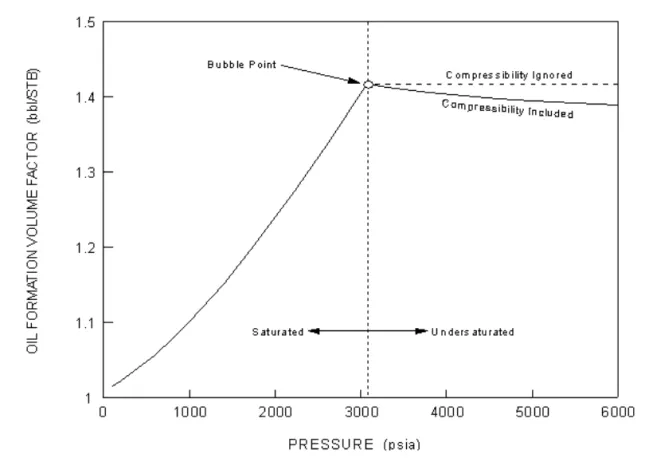
Figure 1.46shows the typical behaviour of the oil formation volume factor that is observed as the system pressure is increased at a constant temperature.
Figure 1.45 Figure 1.46
From the initial pressure up to the bubble point pressure (i.e., the point at which GOR = Rs, which happens to be 3,073 psia in this case), the oil is assumed to be saturated, and Bo continues to increase, as more and more gas goes into solution. The effect of this increasing solution gas is always much greater than the corresponding shrinkage of the oil due to pure compression effects.
At the bubble point, there is no more gas to go into the solution, and the oil then becomes progressively more undersaturated with increasing pressure. With the solution gas-oil ratio being constant, the portion of the curve in Figure 1.46 labelled “Compressibility Ignored” shows the behaviour that would be predicted by the correlations for Bo that we have looked at to this point. In actual fact, however, at pressures greater than the bubble point pressure, Bo is decreasing, due totally to the compressibility of the oil. The actual behaviour that is observed is thus indicated in Figure 1.46by the portion of the curve labelled
“Compressibility Included”.
In general, the compressibility of liquids tends to be relatively low, and the pressure effect on Bo is thus not large. In this particular case, Bo decreases from 1.417 at the bubble point pressure to 1.389 at a pressure of 6,000 psia, which represents a volume decrease of only about 2% for a pressure increase of almost 50%. For some fluid systems, however, particularly lighter oils with relatively high GOR values, the effect can be significantly larger.
Gas Viscosity
Viscosity is a measure of resistance to flow of or through a medium. As a gas is heated, the molecules' movement increases and the probability that one gas molecule will interact with another increases. This translates into an increase in intermolecular activity and attractive forces. The viscosity of a gas is caused by a transfer of momentum between stationary and moving molecules. As temperature increases, molecules collide more often and transfer a greater amount of their momentum. This increases the viscosity.
You can select one of the following calculation methods to calculate the gas viscosity:
• Lee, Gonzalez and Eakin
• Carr, Kobayashi and Burrows (Dempsay version) • Carr, Kobayashi and Burrows (Dranchuk version)
Live Oil Viscosity
Live oil viscosity is the measure of flow resistance of the live oil. Live oil refers to oil that is in equilibrium with any gas that may be present. If there is any free gas, the oil is also said to be saturated. If there is no free gas, but more could go into solution in the oil if it were present, the oil is said to be undersaturated.
You can select one of the following calculation methods to calculate the live oil viscosity:
• Chew and Connally • Beggs and Robinson • Khan
Undersaturated Oil Viscosity
For a given temperature, an oil is said to be undersaturated at any pressure above the bubble point pressure. Increasing the pressure would force more gas to go into solution if there was any, but above the bubble point pressure, there is no more free gas. With no more gas going into solution above the bubble point, the viscosity of the oil actually begins to increase with increasing pressure due to the compressibility of the oil. Since liquid compressibility is typically small, the effect of pressure on viscosity is much smaller above the bubble point than below.
A number of correlations have been proposed for computing the viscosity of undersaturated oils, and a few of these are described below. All of these procedures assume that the bubble point pressure is known at the temperature of interest, as well as the saturated oil viscosity corresponding to the bubble point pressure.
You can select one of the following calculation methods to compute the undersaturated oil viscosity:
• Vasquez and Beggs • Beal
• Khan
• Abdul and Majeed
Dead Oil Viscosity Equation
The term Dead Oil refers to oil that has been taken to stock tank conditions and contains no dissolved (i.e., solution) gas. Dead oil may exist at any pressure or temperature, but it is always assumed that all gas was removed at stock tank conditions. Any properties ascribed to a dead oil are thus characteristic of the oil itself.
Dead Oil Viscosity is the viscosity of an oil with no gas in solution. A number of the more useful methods for calculating this quantity are defined in the equations below.
The General Equation is defined as,
where: µdo = dead oil dynamic viscosity, cP CEPT, SLP = constants for a given oil T = oil temperature, °F
The ASTM Equation is defined as,
where: Z = νdo + 0.7
νdo = dead oil kinematic viscosity, cS
A, B = constants for a given oil T = oil temperature, °F (1.19) (1.20) µdo CEPT 100 T --- SLP =
The kinematic viscosity, νdo is given by,
where: ρo = density of the oil at the temperature of interest, expressed in g/ cm3.
The Eyring Equation is given by,
where: A and B = constants for a given oil
Watson K Factor
You can choose to specify the Watson K Factor, or you can have HYSYS calculate the Watson K Factor. The default option is Specify.
The Watson K Factor is used to characterize crude oils and crude oil fractions. It is defined as,
where: K = Watson K factor
TTB = normal average boiling point for the crude oil or crude oil fraction, °R
SGo = specific gravity of the crude oil or crude oil fraction
(1.21) (1.22) (1.23) νdo µdo ρo ---= νdo Aexp 1.8B T+460 --- = K TB 1 3⁄ SGo ---=
For example, a particular kerosene cut, obtained over the boiling point range 284 - 482 °F, has a specific gravity of 0.7966. Then,
Values of K typically range from about 11.5 to 12.4, although both lower and higher values are observed. In the absence of a known value, K = 11.9 represents a reasonable estimate.
Surface Tension
Surface tension is the measure of attraction between the surface molecules of a liquid. In porous medium systems (i.e. oil reservoirs), surface tension is an important parameter in the estimation of
recoverable reserves because of its effect on residual saturations. On the other hand, most correlations and models for predicting two phase flow phenomena in pipelines are relatively insensitive to surface tension, and one can generally use an average value for calculation purposes. Calculations for wells have a somewhat stronger dependence on surface tension, in that this property can be important in predicting bubble and droplet sizes (maximum stable droplet size increases as surface tension increases), which in turn, can significantly influence the calculated pressure drop. Even then, however, surface tension typically appears in the equations raised to only about the ¼ power.
You can choose to have the surface tension calculated by HYSYS, or you can specify the surface tension. The default option is Calculate.
(1.24) K [0.5 284( +482)+460] 1 3⁄ 0.7966 ---11.86 = =
A.2 References
1 Abbot, M. M., Kaufmann, T. G., and Domash, L., "A Correlation for Predicting
Liquid Viscosities of Petro-leum Fractions", Can. J. Chem. Eng., Vol. 49, p. 379, June (1971).
2 Abdul-Majeed, G. H., and Salman, N. H., "An Empirical Correlation for Oil FVF
Prediction", J. Can. Petrol. Technol., Vol. 27, No. 6, p. 118, Nov.-Dec. (1988).
3 Abdul-Majeed, G. H., Kattan, R. R., and Salman, N. H.,"New Correlation for
Estimating the Viscosity of Under-saturated Crude Oils", J. Can. Petrol.Technol., Vol. 29, No. 3, p. 80, May-June (1990.)
4 Al-Marhoun, M. A., "Pressure-Volume-Temperature Correlations for Saudi
Crude Oils", paper No. SPE 13718, presented at the Middle East Oil Tech. Conf. and Exhib., Bahrain (1985)
5 Al-Marhoun, M. A., "PVT Correlations for Middle East Crude Oils", J. Petrol.
Technol., p. 660, May (1988).
6 Al-Marhoun, M. A., "New Correlations for Formation Volume Factors of Oil
and Gas Mixtures", J. Can. Petrol. Technol., Vol. 31, No. 3, p. 22 (1992).
7 American Gas Association, "Compressibility and Supercompressibility for
Natural Gas and Other Hydrocarbon Gases", Transmission Measurement Committee Report No. 8, December 15 (1985).
8 American Petroleum Institute, API 44 Tables: Selected Values of Properties of
Hydro-carbons and Related Compounds, (1975).
9 Asgarpour, S., McLauchlin, L., Wong, D., and Cheung, V.,
"Pressure-Volume-Temperature Correlations for Wes-tern Canadian Gases and Oils", J. Can. Petrol. Technol., Vol. 28, No. 4, p. 103, Jul-Aug (1989).
10Baker, O., and Swerdloff, W., "Finding Surface Tension of Hydrocarbon
Liquids", Oil and Gas J., p. 125, January 2 (1956).
11Beal, C., "The Viscosity of Air, Water, Natural Gas, Crude Oil and its Associated
Gases at Oil Field Temperatures and Pressures", Trans. AIME, Vol. 165, p. 94 (1946).
12Beg, S. A., Amin, M. B., and Hussain, I., "Generalized Kinematic
Viscosity-Temperature Correlation for Undefined Petroleum Fractions", The Chem. Eng. J., Vol. 38, p. 123 (1988).
13Beggs, H. D., and Robinson, J. R., "Estimating the Viscosity of Crude Oil
14Bradley, H.B. (Editor-in-Chief), Petroleum Engineering Handbook, Society of
Petrol. Engrs (1987); Smith, H.V., and Arnold, K.E., Chapter 19 "Crude Oil Emulsions".
15Carr, N. L., Kobayashi, R., and Burrows, D. B., "Viscosity of Hydrocarbon
Gases Under Pressure", Trans. AIME, Vol. 201, p. 264 (1954).
16Chew, J., and Connally, C. A., "A Viscosity Correlation for Gas Saturated Crude
Oils", Trans. AIME, Vol. 216, p. 23 (1959).
17Dean, D. E., and Stiel, L. I., "The Viscosity of Nonpolar Gas Mixtures at
Moderate and High Pressures", AIChE J., Vol. 11, p. 526 (1965).
18Dempsey, J. R., "Computer Routine Treats Gas Viscosity as a Variable", Oil and
Gas J., p. 141, August 16 (1965).
19Dokla, M. E., and Osman, M. E., "Correlation of PVT Properties for UAE
Crudes", SPE Form. Eval., p. 41, Mar. (1992).
20Dranchuk, P.M., Purvis, R.A., and Robinson, D.B., "Computer Calculations of
Natural Gas Compressibility Factors Using the Standing and Katz Correlations", Inst. of Petrol. Technical Series, No. IP74-008, p. 1 (1974).
21Dranchuk, P. M., and Abou-Kassem, J. H., "Calculations of Z Factors for
Natural Gases Using Equa-tions of State", J. Can. Petrol. Technol., p. 34, July-Sept. (1975).
22Dranchuk, P. M., Islam, R. M. , and Bentsen, R. G., "A Mathematical
Representation of the Carr, Kobayashi, and Burrows Natural Gas Viscosity Cor-relations", J. Can. Petrol. Technol., p. 51, January (1986).
23Elsharkawy, A. M., Hashem, Y. S., and Alikan, A. A., Compressibility Factor for
Gas-Condensates", Paper SPE 59702, presented at the SPE Permian Basin Oil and Gas Recovery Conf., Midland, TX, March (2000).
24Eyring, H., "Viscosity, Plasticity and Diffusion as Examples of Absolute
Reaction Rates", J. Chem. Phys., Vol. 4, p. 283 (1936).
25Gas Processors Association, Engineering Data Book, Tulsa, Oklahoma, 9th
Edition (1977), 10th Edition (1987).
26Glasø, Ø., "Generalized Pressure-Volume-Temperature Correlations", J.
Petrol. Technol., p. 785, May (1980).
27Gomez, J. V., "Method Predicts Surface Tension of Petroleum Fractions", Oil
and Gas J., p. 68, December 7 (1987).
28Gray, H. E., "Vertical Flow Correlation - Gas Wells", API Manual 14 BM,
Second Edition, Appendix B, p. 38, American Petroleum Institute, Dallas, Texas, January (1978).
29Gregory, G. A., "Viscosity of Heavy Oil/Condensate Blends", Technical Note