Assessment of scale dependent function in reef fish, and application to the evaluation of coral reef resilience

Full text

(1)ResearchOnline@JCU. This file is part of the following reference:. Nash, Kirsty L. (2014) Assessment of scale dependent function in reef fish, and application to the evaluation of coral reef resilience. PhD thesis, James Cook University.. Access to this file is available from:. http://researchonline.jcu.edu.au/41029/ The author has certified to JCU that they have made a reasonable effort to gain permission and acknowledge the owner of any third party copyright material included in this document. If you believe that this is not the case, please contact [email protected] and quote http://researchonline.jcu.edu.au/41029/.

(2) Assessment of scale dependent function in reef fish, and application to the evaluation of coral reef resilience. Thesis submitted by Kirsty L. Nash BSc (Hons), MAppSci, MEd in July 2014. for the degree of Doctor of Philosophy within the ARC Centre of Excellence for Coral Reef Studies James Cook University Townsville, Queensland, Australia.

(3) Acknowledgements I would not have started my PhD, let alone finished it, without the enthusiasm and support of Nick Graham. He guided me through the process from ideas to production, and I am extremely grateful for the time he spent helping to keep my stress levels within manageable bounds, whilst at the same time encouraging me to achieve more and attack a wider array of challenges than I would have ever done unaided. I would also like to thank Dave Bellwood for keeping my feet firmly planted in reality when I was designing studies, for the discussions that expanded my understanding, improved my manuscripts and made me laugh, and for giving me the highest accolade of my academic career to date “you write like a Yorkshire lass”. In addition to my supervisors, I have been lucky enough to collaborate with a fantastic range of scientists from a diverse array of backgrounds that helped me stretch my thinking: Craig Allen, David Angeler, Chris Barichievy, Tarsha Eason, Ahjond Garmestani, Dean Grantholm, Melinda Knutson, John Nelson, Magnus Nystrom, Craig Stow, Shana Sundstrom, Justin Welsh and Shaun Wilson. Thank you to Jill Baron at the USGS Powell Centre for facilitating many of these collaborations. Members of the Graham lab and Bellwood lab have acted as great sounding boards through the course of my PhD. Karen Chong-Seng, in particular, has been my PhD companion and I am very grateful for her laughs, stats knowledge and friendship. My fieldwork, and attendance at conferences and workshops has been supported through grants from the Great Barrier Reef Marine Park Authority, the Fish Society of the British Isles, James Cook University, the Great Barrier Reef Foundation, the USGS Powell Centre, and the GDRI. In addition, there have been a number of people that helped me prepare for field work, including: Ross Barrett who made the beautiful wheels that drove Chapter 5, Darren Coker, Andy Hoey and Justin Welsh who provided useful information on Lizard Island reefs, Phil Osmond for all things boating and diving, and Erin at Remote Area Dive. In the field I have been lucky to work with some great people: Nick Graham, Karen Chong-Seng, Fraser Januchowski-Hartley, James Tan and Shaun Wilson. Thank you for the enthusiasm, ideas and problem solving skills. Thank you also to Anne and Lyle at the Lizard Island Research Station, and Jan Robinson previously of the Seychelles Fishing Authority for facilitating my fieldwork. None of the logistical aspects of this thesis would have happened without the phenomenal staff in the CoE for Coral Reef Studies: Olga Bazaka, Jenny Lapin, Louise Lennon, i.

(4) Janet Swanson, Rose-Marie Vasiljuk and David Yellowlees. Thank you also to the great IT department Gordon Bailey, Andrew Norton, and Malcolm Goon Chew for preventing computer melt downs and keeping my data safe. This thesis has been improved immeasurably through discussions on: statistics with Georgie Gurney, Cindy Huchery, Sally Keith, Aaron MacNeil, and Shaun Wilson; ideas and editing with Adrian Arias, Pip Cohen, Louisa Evans, Joana Figueiredo, Christina Hicks, Rebecca Lawton, Dominique McCowan, Chiara Pisapia, Jan Robinson, Jodie Rummer and Silent J. Thank you also to those who encouraged my more creative side projects: Kate Green, Mel Hamel & Erika Woolsey. My PhD is just the latest step in an academic journey, and no acknowledgements would be complete without mentioning those people that got me to this point: Bette Willis my Masters supervisor, Ken Collins my Honours supervisor, Miss Hicks at Downe House and Mr Keep at Ashfold. Mr Keep, you will be pleased to know I have stopped destroying lab equipment. There are a number of friends that have always inspired me with their scientific creativity and passion, in particular Even Moland, Alf Ring Kleiven, Charlie Stalvies, Stephen Taylor and Kellie Watson, I am grateful for your pep talks and enthusiasm. Away from my desk, Erica Blumer, Adriana Chacon, Kate Green, Heidi Moland, Iony Woolaghan, El Mundo, Outer Limits and Swim Squad have helped me maintain perspective, thank you. Finally, I would like to thank my family: M&D for all the support you have shown me over the years, even when the path I have followed has seemed a bit circuitous at times, I value your advice more than you know; G for always providing your honest opinion; S and the Markeys for your encouragement; and A&Gr for thinking having a marine biologist for an aunt is so cool! P, you have kept me sane, reminding me that there is more to life than my thesis, and most of all thank you for making me smile.. ii.

(5) Statement of the contribution of others This thesis includes collaborative work with my supervisors Dr. Nicholas Graham and Prof. David Bellwood, as well as with Dr. Shaun Wilson, Dr. F. Januchowski-Hartley, Justin Welsh, Dr. Craig Allen, Dr. Chris Barichievy, Dr. Magnus Nyström, Shana Sundstrom, Dr. David Angeler, Dr. Tarsha Eason, Dr. Ahjond Garmestani, Dean Granholm, Dr. Melinda Knutson, Dr. John Nelson and Dr. Craig Stow. I led these collaborations and was responsible for project design, data collection, analysis and interpretation of data. My co-authors provided intellectual guidance, assistance with fieldwork, equipment, technical and editorial assistance and financial support. For the quantitative review in Chapter 2 (home range allometry), Justin Welsh also participated in project design, data collection and writing of the introduction. This project was funded from a range of sources. Funding for Kirsty Nash was derived from a Science for Management Award from the Great Barrier Reef Marine Park Authority, the 2011 JCU “my research in 3 minutes” award, the 2013 Bommies Award from the Great Barrier Reef Foundation, a travel award from the Fish Society of the British Isles, and working group funding from the US Geological Survey Powell Centre. Funding for Nicholas Graham came from a Queensland Smart Futures award and Australian Research Council grants.. An. Australian Postgraduate Award provided stipend and tuition support. Every reasonable effort has been made to gain permission and acknowledge the owners of copyright material. I would be pleased to hear from any copyright owner who has been omitted or incorrectly acknowledged.. iii.

(6) Abstract In response to the anthropogenic pressures affecting ecosystems, and the resultant habitat and community changes these impacts cause, there has been increasing interest in using resilience approaches to study ecosystems. The resilience of a system its capacity to adapt to changing conditions whilst maintaining core processes, and resisting shifts to different regimes. Thus, the resilience concept allows the state of a system to be thought about within a dynamic, ecosystem-based framework.. Despite this interest in resilience approaches, quantitative. indicators of ecosystem resilience are rarely tested.. Understanding and quantifying the. functional roles played by species, and thus their importance in driving key ecosystem processes, has been suggested as one approach for quantifying resilience. In the context of coral reefs, herbivory by reef fishes has been identified as an important process controlling algae and supporting coral dominance. As a result, there is an extensive literature characterising how herbivorous species provide their function. However, there has been little evaluation of the spatial scales over which fish perform their functional roles. Knowledge of the scales over which fishes provide their function may be used to develop a broader indicator of resilience: cross-scale redundancy. The cross-scale resilience model, first proposed by Peterson et al. in 1998, suggests that the scale at which an individual provides its function will influence its response to scale-specific disturbances. Thus, the presence of species operating at different scales within a community (cross-scale redundancy), should be a useful indicator of resilience. Implementation and testing of cross-scale redundancy on coral reefs would go some way to addressing the need for empirical testing of resilience indicators. To test these indicators, this thesis is split into two parts: in Part 1 (Chapter 2-5) I evaluate the spatial scales at which fish interact with the reef and provide their function; in Part 2 (Chapter 6-8) I investigate the application of the cross-scale resilience model in the context of coral reefs. The knowledge developed in Part 1 is essential for assessing the appropriateness of implementing the cross-scale resilience model for reef fish because these chapters test the underlying assumptions of the model used in Part 2. The relationship between body size and home range provides a useful way of summarising the spatial scales at which communities of fish operate. In Chapter 2 I performed a quantitative review of studies examining home range in reef fishes, and assessed the interspecific relationship between body mass and home range area. Body mass and home range were positively related. Fishes appeared to occupy a smaller area per unit mass than terrestrial iv.

(7) vertebrates. When the small home ranges of reef fish are considered in concert with their apparent reluctance to cross open areas, it suggests that reserves aimed at protecting fish biodiversity may be more effective if located across whole reefs as home ranges are less likely to cross reserve boundaries. Home ranges may include areas that are used for activities such as sleeping, rather than focusing on those locations where the organism is providing the core functions of interest, such as grazing. Therefore, in Chapter 3 I assessed the allometric relationship between small-scale foraging movements and body size for herbivorous reef fishes within the functional groups: browsers, farmers, grazer/detritivores, and scraper/excavators.. The relationship between. vulnerability of species to fishing and their scale of foraging was also examined. I found evidence of a strong, positive, log linear relationship between scale of foraging movement and fish length. Some functional groups, such as scrapers/excavators, performed their role over a wide range of scales, whereas browsers were represented by few species and operated over a much narrower range of scales. Overfishing is likely to not only remove species operating at large scales, but also the browser group as a whole. The spatial scales at which fish operate are not only affected by life history traits such as body size, they are also shaped by the habitats available to the individual. In Chapter 4, I assessed the influence of among-site variation in habitat condition on the short-term foraging range of two species of parrotfish. The primary predictor of these foraging movements was coral cover. The study suggests that future changes in coral cover are likely to alter the way reef herbivores forage. Habitat condition may also drive the underlying body size distribution of fish communities. In Chapter 5 I characterized patterns of cross-scale habitat complexity, and examined how this related to body-depth abundance distributions of associated fish assemblages over corresponding spatial scales. I found that reefs formed from different underlying substrata exhibit distinct patterns of cross-scale habitat complexity and this is reflected in the fish body depth distributions. The second part of the thesis used knowledge generated in Part 1 to test the applicability of Peterson et al.’s cross-scale resilience model on coral reefs. This model was developed from the discontinuity hypothesis, which explores inherent scales of structure within ecosystems. In Chapter 6 I reviewed the conceptual framework underlying discontinuities.. The chapter. explored the utility of discontinuities for understanding cross-scale patterns by describing recent advances in examining non-linear responses to disturbance, and phenomena such as invasions, and resilience. I detailed outstanding knowledge gaps, in particular pertaining to the implementation of the cross-scale resilience model for taxa with indeterminate growth such as reef fishes. v.

(8) To address the issue of applying the cross-scale resilience model to species with indeterminate growth, in Chapter 7 I performed a comparison of bird (determinate growth) and fish (indeterminate growth) body mass distributions, assessing the respective suitability of distinct analytical approaches for understanding habitat-size relationships in different ecosystems. I evaluated three size distribution indices: species size relationships, species sizedensity relationships and individual size-density relationships, and two types of analysis: looking for either discontinuities or abundance modes in the distributions. All the indices and analyses were useful for examining the relationship between habitat structure and size for species with determinate growth. In contrast, for species with indeterminate growth, such as fishes, individual size-density relationships were more useful. Finally, in Chapter 8 I applied the cross-scale resilience model on coral reefs. I assessed the effectiveness of cross-scale redundancy in herbivores as an indicator of response diversity and benthic recovery on reefs monitored through a coral bleaching event.. The. distribution (redundancy) of herbivores operating across a broader range of spatial scales prior to the bleaching corresponded with increased reef recovery post-disturbance, as proposed by the cross-scale resilience model. Analysis of the change in biomass across size classes indicated that response diversity, with declines in small herbivores and increases in large herbivores, enhanced the overall herbivore biomass at recovering sites. My research characterized the spatial ecology of reef fish communities, and herbivores in particular.. This knowledge was used to underpin the testing of a potential resilience. indicator: the cross-scale resilience model; a model that proved to be effective in the context of coral reefs. Critically, my research provides fundamental knowledge regarding the function provided by coral reef fishes, highlighting the spatial scales over which management is needed to support their critical functions. These results will help managers to predict the relative likelihood of different reefs declining or recovering following severe disturbances. Understanding the spatial ecology of fishes may hold the key to the management of coral reef recovery in the future.. vi.

(9) Table of Contents ACKNOWLEDGEMENTS STATEMENT OF THE CONTRIBUTION OF OTHERS ABSTRACT. III. IV. TABLE OF CONTENTS LIST OF TABLES LIST OF FIGURES CHAPTER 1:. I. GENERAL INTRODUCTION. VII XI XIII 1. 1.1. THE IMPORTANCE OF FUNCTIONAL DIVERSITY ................................................ 1. 1.2. BODY SIZE AS A PROXY FOR SPATIAL SCALE ..................................................... 2. 1.3. ALLOMETRY OF HOME RANGE ................................................................................ 2. 1.4. ALLOMETRY OF FUNCTIONAL MOVEMENTS ...................................................... 3. 1.5. MOVEMENT AND HABITAT EFFECTS ..................................................................... 3. 1.6. BODY SIZE DISTRIBUTIONS AND HABITAT EFFECTS ........................................ 4. 1.7. ASSESSMENT OF CORAL REEF RESILIENCE ......................................................... 4. 1.8. AIMS AND THESIS OUTLINE ..................................................................................... 6. CHAPTER 2:. HOME RANGE ALLOMETRY IN CORAL REEF FISHES: COMPARISON TO OTHER VERTEBRATES, METHODOLOGICAL ISSUES AND MANAGEMENT APPLICATIONS 9. 2.1. ABSTRACT ..................................................................................................................... 9. 2.2. INTRODUCTION............................................................................................................ 9. 2.3. MATERIALS AND METHODS ................................................................................... 11. 2.4. RESULTS ...................................................................................................................... 13. 2.5. DISCUSSION ................................................................................................................ 20. 2.5.1 2.5.2 2.5.3 2.5.4 2.5.5. Evolution in home range methods .................................................................................. 20 Home range allometry in reef fishes and effects of tracking method ............................. 21 Comparisons in home range allometry across taxa ....................................................... 22 Management and ecological implications...................................................................... 23 Conclusions and future directions.................................................................................. 24. CHAPTER 3:. FISH FORAGING PATTERNS, VULNERABILITY TO FISHING AND IMPLICATIONS FOR THE MANAGEMENT OF ECOSYSTEM FUNCTION ACROSS SCALES 26. 3.1. ABSTRACT ................................................................................................................... 26. 3.2. INTRODUCTION.......................................................................................................... 27. 3.3. METHODS .................................................................................................................... 30 vii.

(10) 3.3.1 3.3.2 3.3.3 3.3.4 3.3.5. Study sites & species ...................................................................................................... 30 Fish and benthic censuses .............................................................................................. 30 Study species .................................................................................................................. 30 Behavioral studies .......................................................................................................... 31 Data analysis .................................................................................................................. 32. 3.4. RESULTS ...................................................................................................................... 33. 3.4.1 3.4.2. Benthic cover and herbivore abundance ........................................................................ 33 Behavioural metrics ....................................................................................................... 35. 3.5. DISCUSSION ................................................................................................................ 39. 3.5.1 3.5.2 3.5.3 3.5.4. Allometric relationships ................................................................................................. 39 Cross-scale patterns ....................................................................................................... 41 Vulnerability of cross-scale patterns to fishing .............................................................. 43 Conclusions 45. CHAPTER 4:. INFLUENCE OF HABITAT CONDITION AND COMPETITION ON FORAGING BEHAVIOUR OF PARROTFISHES 46. 4.1. ABSTRACT ................................................................................................................... 46. 4.2. INTRODUCTION.......................................................................................................... 46. 4.3. MATERIALS AND METHODS ................................................................................... 49. 4.3.1 4.3.2 4.3.3 4.3.4 4.3.5. Study sites 49 Study species .................................................................................................................. 49 Behavioural studies ........................................................................................................ 50 Fish and benthic censuses .............................................................................................. 51 Data analysis .................................................................................................................. 51. 4.4. RESULTS ...................................................................................................................... 53. 4.4.1 4.4.2 4.4.3 4.4.4. Site-specific benthic cover and fish abundance ............................................................. 53 Inter-foray distance ........................................................................................................ 53 Short-term foraging range ............................................................................................. 54 Shape of short-term foraging range ............................................................................... 57. 4.5. DISCUSSION ................................................................................................................ 59. 4.5.1 4.5.2 4.5.3 4.5.4. Habitat condition ........................................................................................................... 59 Predation risk ................................................................................................................. 61 Competition 61 Broader implications ...................................................................................................... 62. CHAPTER 5:. CROSS-SCALE HABITAT STRUCTURE DRIVES FISH BODY SIZE DISTRIBUTIONS ON CORAL REEFS 64. 5.1. ABSTRACT ................................................................................................................... 64. 5.2. INTRODUCTION.......................................................................................................... 64. 5.2.1 5.2.2 5.2.3. Analytic framework ........................................................................................................ 65 Theoretical framework ................................................................................................... 68 Aims 68. 5.3. METHODS .................................................................................................................... 69. 5.3.1 5.3.2 5.3.3. Materials 69 Field methods ................................................................................................................. 69 Data analysis .................................................................................................................. 70 viii.

(11) 5.4. RESULTS ...................................................................................................................... 72. 5.4.1 5.4.2 5.4.3. Benthic community and habitat classification................................................................ 72 Cross-scale habitat complexity ...................................................................................... 72 Fish individual body depth distributions ........................................................................ 73. 5.5. DISCUSSION ................................................................................................................ 75. 5.5.1 5.5.2 5.5.3 5.5.4. Evaluation of the textural discontinuity hypothesis ....................................................... 75 Fish body depth distributions ......................................................................................... 77 Cross-scale habitat complexity ...................................................................................... 78 Conclusions 80. CHAPTER 6:. DISCONTINUITIES, CROSS-SCALE PATTERNS AND THE ORGANIZATION OF ECOSYSTEMS. 81. 6.1. ABSTRACT ................................................................................................................... 81. 6.2. INTRODUCTION.......................................................................................................... 81. 6.3. DISCONTINUITIES: FRAMEWORK, EVIDENCE AND EXTENSIONS................. 83. 6.3.1 6.3.2 6.3.3. Conceptual framework ................................................................................................... 83 Modeling and empirical evidence .................................................................................. 86 Extensions to original framework .................................................................................. 88. 6.4. APPLICATIONS OF DISCONTINUITY ANALYSIS................................................. 90. 6.4.1 6.4.2 6.4.3 6.4.4. Identification of scales ................................................................................................... 90 Identification of nonlinearities and regime shifts........................................................... 91 Functional distributions, macroecology and resilience ................................................. 93 Extinctions and invasions ............................................................................................... 96. 6.5. FUTURE DIRECTIONS................................................................................................ 97. CHAPTER 7:. HABITAT STRUCTURE AND BODY SIZE DISTRIBUTIONS: CROSSECOSYSTEM COMPARISON FOR TAXA WITH DETERMINATE AND INDETERMINATE GROWTH 99. 7.1. ABSTRACT ................................................................................................................... 99. 7.2. INTRODUCTION........................................................................................................ 100. 7.3. MATERIALS AND METHODS ................................................................................. 104. 7.3.1. Data analysis ................................................................................................................ 106. 7.4. RESULTS .................................................................................................................... 110. 7.4.1 7.4.2 7.4.3 7.4.4. Analysis 1: discontinuity patterns across species size relationships (SSRs) ................ 110 Analysis 2: abundance patterns across species size-density relationships (SSDRs).... 112 Analysis 3: discontinuity patterns across individual size-density relationships (ISDRs) 114 Analysis 4: abundance patterns across individual size-density relationships (ISDRs) 114. 7.5. DISCUSSION .............................................................................................................. 115. 7.5.1 7.5.2 7.5.3. Body size distributions: choice of index and analysis .................................................. 116 Size and vulnerability ................................................................................................... 119 Conclusions and future directions................................................................................ 120. CHAPTER 8:. HERBIVORE CROSS-SCALE REDUNDANCY SUPPORTS RESPONSE DIVERSITY AND CORAL REEF RECOVERY. 121 ix.

(12) 8.1. ABSTRACT ................................................................................................................. 121. 8.2. INTRODUCTION........................................................................................................ 122. 8.3. METHODS .................................................................................................................. 125. 8.3.1 8.3.2. Field methods ............................................................................................................... 125 Data analysis ................................................................................................................ 126. 8.4. RESULTS .................................................................................................................... 130. 8.4.1 8.4.2 8.4.3 8.4.4. Benthic condition ......................................................................................................... 130 Redundancy as an indicator of reef resilience ............................................................. 131 Redundancy as an indicator of response diversity ....................................................... 132 Redundancy over time .................................................................................................. 135. 8.5. DISCUSSION .............................................................................................................. 137. 8.5.1 8.5.2 8.5.3. Redundancy as an indicator of response diversity and reef resilience ........................ 137 Redundancy over time .................................................................................................. 138 Management implications ............................................................................................ 139. CHAPTER 9:. GENERAL DISCUSSION. 141. 9.1. CONTRIBUTIONS TO METHODOLOGY ............................................................... 143. 9.2. MANAGEMENT IMPLICATIONS ............................................................................ 144. 9.3. FUTURE RESEARCH DIRECTIONS ........................................................................ 145. CHAPTER 10: REFERENCES. 147. APPENDIX A: SUPPLEMENTAL INFORMATION FOR CHAPTER 2. 180. APPENDIX B: SUPPLEMENTAL INFORMATION FOR CHAPTER 3. 185. APPENDIX C: SUPPLEMENTAL INFORMATION FOR CHAPTER 4. 195. APPENDIX D: SUPPLEMENTAL INFORMATION FOR CHAPTER 6. 200. APPENDIX E: SUPPLEMENTAL INFORMATION FOR CHAPTER 7. 204. APPENDIX F: SUPPLEMENTAL INFORMATION FOR CHAPTER 8. 214. APPENDIX G: PUBLICATIONS ARISING DURING CANDIDATURE. 220. x.

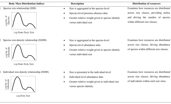
(13) List of Tables Table 2-1: Comparison of random effect structures for models that either A) included tracking method or B) did not include tracking method in the analysis................................. 15 Table 2-2: Set of candidate models compared using AICc values to determine the best-fit fixed structure, for models that either A) included tracking method or B) did not include tracking method in the analysis. ............................................................................... 16 Table 2-3: Coefficients of the best-fit fixed models exploring the relationship between log home range and log body size for models that either A) included tracking method or B) did not include tracking method in the analysis. Only those models within 2AICc value of the optimal model are presented. .................................................... 17 Table 3-1: A) Density of fish (100m-2 ±SE) within the four herbivorous functional groups at each site, and B) the proportion of functional group abundance represented by species assessed for foraging metrics and included in Fig. 3-2. Data based on UVC counts, pooled to site level, and incorporating all size classes. ............................... 34 Table 3-2: Summary of scaling parameters for the relationship between body length and A) Intra-foray distance, and B) Inter-foray distance, where parameters represent y=αxβ. .................................................................................................................................. 35 Table 4-1: Best-fit models for predicting inter-foray group distance of A) Scarus niger and B) Scarus frenatus. Models presented are those with lowest AICc values from GAMM and GLMM that evaluate the influence of exposure, structural complexity, coral cover, EAM cover, parrotfish abundance and large piscivore abundance. Significant predictors are in bold (α = 0.01)............................................................................... 54 Table 4-2: Best-fit models for predicting shape of foraging range (compactness ratio) of A) Scarus niger and B) Scarus frenatus. Models presented are those with lowest AICc values from GAMM that evaluate the influence of exposure, structural complexity, coral cover, EAM cover, parrotfish abundance and large piscivore abundance. Significant predictors are in bold (α = 0.01). ........................................................... 56 Table 5-1: Expected relationships between cross-scale patterns of habitat complexity and associated fish body depth distributions. ................................................................. 67 Table 5-2: Analysis of similarity (ANOSIM) among sites of different habitat type. ................ 73 Table 5-3: Results of Monte-Carlo simulation of differences in fractal dimension among sites and scales for each habitat........................................................................................ 75 Table 6-1: Glossary of terms. ..................................................................................................... 84 Table 6-2: Practical tools for detecting discontinuities. Several methods have been described for identifying discontinuities and multi-modality within the distributions of variables such as body size or biomass. The suitability of these methods varies with respect to the type of data available and the research question. All techniques have their biases (reviewed in Stow, Allen & Garmestani 2007), therefore a combination of methods, followed by triangulation of their respective results, has been identified as the most robust approach. To date mean body mass has been primarily used as a measure of body size, though for species with indeterminate growth other metrics may be more appropriate. The list of platforms specified is not exhaustive. ........... 89 Table 7-1: Different indices of body size distribution considered in this study. Key features and their value in examining the distribution of resources within communities are presented. ............................................................................................................... 101 xi.

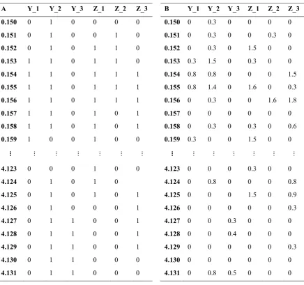
(14) Table 7-2: Combinations of the three size distribution indices and two analytical approaches used in the four analyses comparing body size distributions among different habitat types. ...................................................................................................................... 105 Table 7-3: Matrix setup for different analyses using example data. Row labels are log 10 body sizes, column titles are habitat type (Y or Z) and site number (1, 2 or 3). A) Analysis 1 (species-level data) and 3 (individual-level data), where data represent discontinuities (0) and aggregations (1) identified by the Gap Rarity Index (GRI), B) Analysis 2 (species-level data) and 4 (individual-level data), where data represent log 10 (abundance +1)............................................................................................ 109 Table 7-4: Analysis of Similarities (ANOSIM) comparing the size distributions of communities for sites of different habitat type for A) Lofty Ranges bird, B) Borneo bird, C) Seychelles fish, and D) Great Barrier Reef fish communities. Analysis 1: Comparison of discontinuities in species mean size relationships (SSRs). Analysis 2: Comparison of abundance in species mean size-density distributions (SSDRs). Analysis 3: Comparison of discontinuities in individual size-density relationships (ISDRs). Analysis 4: Comparison of abundance across individual size-density relationships (ISDRs). The resemblance matrices were calculated using Euclidean distances for Analyses 1 and 3, and chord distances for Analyses 2 and 4............ 111 Table 8-1: Description of the two sets of redundancy metrics used in the analyses. ............... 127 Table 8-2: Model selection comparing the utility of the different redundancy metrics in 1994 as predictors of reef benthic trajectories from 2005 to 2011. A) Step 1 evaluated the performance of the metrics from the functional group and the functional & size approaches, and B) Step 2 evaluated the performance of models combining different metrics arising from the functional & size approach. ............................................ 132 Table 8-3: Models of relationships between herbivore biomass in the different years and A) functional & size dispersion, and B) functional & size evenness. Significant relationships are shown in bold. Herbivore biomass was square root transformed to meet model assumptions. ....................................................................................... 134. xii.

(15) List of Figures Figure 1-1: Relationship between the cross-scale resilience model (red), required knowledge on the functional role of species (green), and the underlying assumptions of the model relating to the spatial ecology of reef fishes (blue). ................................................... 6 Figure 2-1: Number of publications documenting home range in coral reef fishes, categorised according to year of publication and A) Tracking method used, B) Detection method of telemetry studies, and C) Analytical method undertaken. ................................... 14 Figure 2-2: Interspecific relationship between log body mass (g) and log home range (m2) for coral reef fishes from studies estimating home ranges using Minimum Convex Polygons (MCPs), for models that A) included tracking method with different intercepts among the two tracking methods and trophic groups, and B) did not include tracking method in the analysis. Symbols: squares & dotted lines – visual tracking; circles & solid lines – telemetry tracking; grey – predators, black – herbivores. ................................................................................................................ 18 Figure 2-3: Comparison of interspecific relationship between log body mass (g) and log home range (m2) among vertebrate taxa. Blue shaded area represents range of intercepts provided by model for reef fish incorporating tracking method; solid blue line – reef fish for model not incorporating tracking method; solid grey line – lake fish (Minns 1995); dashed grey line – river fish (Minns 1995); solid black line – birds (Schoener 1968 recalculated in Harestad & Bunnell 1979); dashed black line – lizards (Turner et al. 1969); dotted black line – mammals (Kelt and Vuren 2001). 19 Figure 3-1: Map of study sites at Lizard Island. Prevailing winds are from the south east. ..... 31 Figure 3-2: Relationship between body length and A) Intra-foray distance or B) Inter-foray distance for herbivorous reef fish, presented in i)log-log scales and ii) backtransformed to arithmetic scales. Lines represent significant relationships (±95% CI) based on OLS regression, showing common slope and intercept among sites for both variables. Symbols indicate functional group: triangle-Farmer, squareGrazer/Detritivore, circle-Browser, cross-Scraper/Excavator.................................. 36 Figure 3-3: Residuals for relationship between body length and A) Intra-foray distance or B) Inter-foray distance for species of herbivorous reef fish. Bars represent mean value across sites where species was observed at multiple sites. Numbers provide mean residual for functional group. Species: Kv-Kyphosus vaigiensis; Nu-Naso unicornis; Dm- Dischistodus melanotus; Dpe- Dischistodus perspicillatus; Dps- Dischistodus psuedochrysopecilus; HpHemiglyphidodon plagiometopon; PlPlectroglyphidodon lacrymatus; Pa- Pomacentrus adelus; Sn- Stegastes nigricans; Ab- Acanthurus blochii; Ana- Acanthurus nigricauda; Ans- Acanthurus nigrofuscus; Ao- Acanthurus olivaceus; Cb- Centropyge bicolor; Cs- Ctenochaetus striatus; Sic- Siganus corallinus; Sid- Siganus doliatus; Sip- Siganus punctatus; Siv- Siganus vulpinus; Zs-Zebrasoma scopas; Zv- Zebrasoma veliferum; CebCetoscarus bicolor; Chm- Chlorurus microrhinus; Chs- Chlorurus sordidus; ScaScarus altipinnis; Scf- Scarus flavipectoralis; Scn- Scarus niger; Sco- Scarus oviceps; Scr- Scarus rivulatus; Scrb- Scarus rubroviolaceus; Scs- Scarus schlegeli. .................................................................................................................................. 37 Figure 3-4: Correlation between vulnerability to fishing pressure (based on index by Cheung et al. 2005), and A) Intra-foray distance (spearman rho= 0.69, p<0.001) or B) Interforay distance (spearman rho= 0.62, p<0.001). Intra-foray and inter-foray data for each species are pooled across sites. Symbols indicate functional group: triangleFarmer, square-Grazer/Detritivore, circle-Browser, cross-Scraper/Excavator. ....... 38 xiii.

(16) Figure 4-1: The relationship between coral cover and inter-foray group distance for a) Scarus niger and b) Scarus frenatus, and with shape of foraging range for c) Scarus niger and d) Scarus frenatus. The data are plotted showing fitted GAM smoothers ± 95% confidence intervals for the best-fit model, identified using AICc values. X axes are percent coral cover, y axes are centred scales showing partial effect of coral cover on foraging metrics in the respective models. Smoothing parameters are 5.49, 1, 2.03 and 2.05, respectively for the four plots. Grey graphics in a) and b) represent relative distances between foray groups, where dots depict foray groups and connecting lines depict inter-foray group distance; grey graphics in c) and d) represent relative shapes of short term foraging range represented by different values of compactness ratio. .................................................................................... 55 Figure 4-2: The relationship between ln parrotfish abundance and shape of foraging range (compactness ratio) for a) Scarus niger and b) Scarus frenatus. The data are plotted showing fitted GAM smoothers ± 95% confidence intervals for the best-fit model, identified using AICc values. X axes are percent coral cover, y axes are centred scales showing partial effect of coral cover on foraging metrics in the respective models. Smoothing parameters are 1 and 2.64, respectively for the two plots. ....... 58 Figure 5-1: Estimation of linear distance by wheels of different diameters. Wheel with small diameter (i) fits into more holes in the reef than mid-sized (ii) or large wheels (iii), thus measuring a greater linear distance (iv). The fractal dimension (D; 1-slope of the log distance against log spatial scale) provides an indication of the availability of refuges of different sizes (complexity across spatial scales).................................... 66 Figure 5-2: A) Mean linear (perceived) distance measured along transects using wheels of different step lengths for i) Coral, ii) Algae, and iii) Granitic sites. Dotted lines represent linear distance along transect (500cm). B) Mean fractal dimension (D) of substrate estimated at different spatial scales for i) Coral, ii) Algae, and iii) Granitic sites. Error bars represent bootstrapped non parametric 95% confidence intervals. Shading indicates location of breaks in D with scale (scale breaks); lowercase letters represent significant groupings assessed using Monte Carlo simulation of mean differences corrected for multiple comparisons. Dotted lines represent fractal dimension for straight Euclidean curve (D= 1). C) Distribution of fish abundance across body depth size classes for i) Coral, ii) Algae, and iii) Granitic sites. Dotted curves represent bootstrapped 95% confidence intervals. Grey and black bars identify locations of significant peaks and troughs in abundance respectively, identified using 95% confidence intervals of bootstrapped second derivates of GAM abundance smoothers. Shading represents location of breaks in abundance identified as modes with significantly different abundances, using Monte Carlo simulation. Note, log scale on x axis represents wheel diameter (cm) in A) and B) and body depth (cm) in C). ...................................................................................... 74 Figure 6-1: Multi-scale relationship between processes occurring over different, discrete spatial and temporal scales, and the resulting discontinuous distribution of an ecosystem attribute, such as physical habitat structure. The distribution of processes over discrete scale ranges, and the landscape patterns they produce represent the ‘intrinsic’ scales (Table 6-1) of a system (adapted from Wiens 1989). Discontinuities, or zones of low or variable resource availability lie between these ‘intrinsic’ scales. ...................................................................................................... 82 Figure 6-2: The relationship between scales of habitat structure and discontinuities in body size distributions. A) Discontinuous hierarchy of scale for structure and resources within a reef ecosystem, from the individual branches of coral colonies to multi-reef scales. B) A discontinuous fish body size distribution. Crosses represent individual species; aggregations (dashed circles) of similarly sized species operate at similar scales, and are separated from neighboring aggregations by discontinuities. Body xiv.

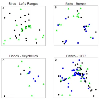
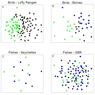
(17) size correlates with scale of perception, such that larger species operate over larger scales. C) Representative species from each of the 5 aggregations. For example the blue spine unicornfish (indicated by *) is a member of aggregation 4, and perceives and interacts with its habitat at the reef scale. (Multireef image courtesy of James Oliver: http://www.reefbase.org; fish vector graphics courtesy of, from right to left, Tracey Saxby, Joanna Woerner, Joanna Woerner, Christine Thurber, and Tracey Saxby: Integration and Application Network, http://ian.umces.edu/imagelibrary/). 85 Figure 6-3: The strength of competitive interactions among species using similar resources at different scales. The range of scales at which birds in different body size aggregations perceive and feed on spruce budworm extend from the crown of a fir to a stand of trees, and these sit within larger spatial scales (forest). Blue arrows represent the relative strength of competitive interactions among these species. When species are located within the same body size aggregation (dashed circles) they forage over similar scales and thus experience relatively strong competitive interactions (thick arrow) compared with species in different body size aggregations that are foraging at different scales (thinner arrows). (Tree aerial photo courtesy of Google Earth, spruce tree image courtesy of Rosendahl, http://www.public-domainimage.com/; chickadee, warbler and robin graphics courtesy of Tracey Saxby: Integration and Application Network, http://ian.umces.edu/imagelibrary/; crow image ©Can Stock Photo Inc. / Birchside). ............................................................. 87 Figure 6-4: A) Patterns of variance in abundance of species located in body mass aggregations. Those species at the centre of aggregations exhibit lower variance in abundance (B), than those at the edges of aggregations (C). N.B. Body size and abundance are used as an example. Other variables may show similar patterns of aggregation and variability. ................................................................................................................ 92 Figure 6-5: Influence of disturbance on the distribution of functional groups across scales. A) The range of scales at which fish perceive, interact with and use resources on the reef, from the individual branches of coral colonies to multi-reef scales. B) Predisturbance: discontinuous fish body size distribution, where crosses represent individual species and colors indicate functional group membership. Colored arrows indicate the range of scales over which each group operates and therefore provides its function: the green functional group operates over a wide range of scales, whereas the red functional group only operates over small scales. C) Postdisturbance: coral disease provides a small scale disturbance that affects fish species operating at the branch and colony scales (empty aggregations). Those functional groups with redundancy across spatial scales (blue, green and purple groups) may compensate for loss of species at these small scales (dashed arrows), whereas those functional groups with low cross-scale redundancy (red group) are reliant on passive links (recruitment) or mobile links (adult fish) recolonizing from neighbouring regions (red dotted arrow) for maintenance of function. (Multireef image courtesy of James Oliver: http://www.reefbase.org). ............................................................. 94 Figure 7-1: Different analytical approaches for evaluating patterns in body size distributions. A) Analysis looks for the presence of discontinuities or gaps (red bar) in size distributions. This approach may be used for either distributions that incorporate abundance information (e.g. ISDRs) or those that do not (SSRs) because abundance information is ignored; the analysis solely searches for gaps in the distribution. B) Analysis evaluates abundance patterns, looking for modes (red bar) and the distribution of abundances across size classes. This approach may only be used for distributions that incorporate abundance information (SSDRs and ISDRs). ......... 103 Figure 7-2: Non-metric multi-dimensional scaling (nMDS) comparing size distributions of communities for sites of different habitat type. Comparison of discontinuities in species size relationships (SSRs; Analysis 1) for A) Lofty Ranges bird, B) Borneo xv.

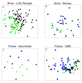
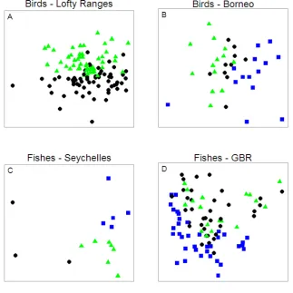
(18) bird, C) Seychelles fish, and D) Great Barrier Reef fish communities. The resemblance matrices were calculated using Euclidean distances. Symbols in A: black circles – gum woodland, green triangles – stringybark woodland; symbols in B: black circles – logged_89 forest, green triangles – logged_93 forest, blue squares – unlogged forest; symbols in C: black circles – algal-dominated carbonate reef, green triangles – coral-dominated carbonate reef, blue squares – granitic reef; symbols in D: black circles – disturbed reef, green triangles – recovering reef, blue squares – undisturbed reef...................................................................................... 112 Figure 7-3: Non-metric multi-dimensional scaling (nMDS) comparing size distributions of communities for sites of different habitat type. Comparison of abundance patterns in species size-density relationships (SSDRs; Analysis 2) for A) Lofty Ranges bird, B) Borneo bird, C) Seychelles fish, and D) Great Barrier Reef fish communities. The resemblance matrices were calculated using chord distances. Symbols in A: black circles – gum woodland, green triangles – stringybark woodland; symbols in B: black circles – logged_89 forest, green triangles – logged_93 forest, blue squares – unlogged forest; symbols in C: black circles – algal-dominated carbonate reef, green triangles – coral-dominated carbonate reef, blue squares – granitic reef; symbols in D: black circles – disturbed reef, green triangles – recovering reef, blue squares – undisturbed reef...................................................................................... 113 Figure 7-4: Non-metric multi-dimensional scaling (nMDS) comparing size distributions of communities for sites of different habitat type. Comparison of discontinuities in individual size-density relationships (ISDRs; Analysis 3) for A) Lofty Ranges bird, B) Borneo bird, C) Seychelles fish, and D) Great Barrier Reef fish communities. The resemblance matrices were calculated using Euclidean distances. Symbols in A: black circles – gum woodland, green triangles – stringybark woodland; symbols in B: black circles – logged_89 forest, green triangles – logged_93 forest, blue squares – unlogged forest; symbols in C: black circles – algal-dominated carbonate reef, green triangles – coral-dominated carbonate reef, blue squares – granitic reef; symbols in D: black circles – disturbed reef, green triangles – recovering reef, blue squares – undisturbed reef...................................................................................... 115 Figure 7-5: Non-metric multi-dimensional scaling (nMDS) comparing size distributions of communities for sites of different habitat type. Comparison of abundance patterns in individual size-density relationships (ISDRs; Analysis 4) for A) Lofty Ranges bird, B) Borneo bird, C) Seychelles fish, and D) Great Barrier Reef fish communities. The resemblance matrices were calculated using chord distances. Symbols in A: black circles – gum woodland, green triangles – stringybark woodland; symbols in B: black circles – logged_89 forest, green triangles – logged_93 forest, blue squares – unlogged forest; symbols in C: black circles – algal-dominated carbonate reef, green triangles – coral-dominated carbonate reef, blue squares – granitic reef; symbols in D: black circles – disturbed reef, green triangles – recovering reef, blue squares – undisturbed reef. ................................. 116 Figure 8-1: A coral reef experiencing high water temperatures driving a bleaching event (illustrated with thermometers). The proposed influence of A) herbivore functional redundancy (multiple species providing the same role) and B) herbivore cross-scale functional redundancy (multiple species providing the same role but at different spatial scales as indicated by variable body sizes; Nash et al. 2013) on community response diversity, leading to either reef recovery or decline. Both communities have the same total herbivore biomass and functional diversity prior to the disturbance. ............................................................................................................ 124 Figure 8-2: Example distribution of species-size groupings in trait space, with relative biomass indicated by bubble size. Individual plots illustrate differences between communities with same number of species and total biomass but exhibiting varying xvi.

(19) levels of dispersion and evenness. For illustrative purposes, only two trait axes are shown. For the metrics calculated solely from the function information, trait axes would be developed from dummy variables representing each functional group. For the metrics calculated from function and size information, trait axes would be body size and dummy variables representing each functional group. In this latter situation, those sites with high dispersion and evenness possess high cross-scale redundancy and functional diversity, whereas those sites with low dispersion and evenness possess low cross-scale redundancy and functional diversity. Those sites with high dispersion but low evenness have high dispersion across trait space, but the low evenness reduces the inherent redundancy. Sites with low dispersion and high evenness have little dispersion across trait space and thus low functional diversity and cross-scale redundancy, but redundancy within the represented trait combinations. ......................................................................................................... 128 Figure 8-3: Principal component analysis of benthic habitat variables in 1994 (circles), 2005 (triangles) and 2011 (crosses). A) Variation in the benthic habitat among sites shown for the first two axes of a principal component analysis. B) Relative contribution of the benthic variables to the variation in benthic condition. ........... 131 Figure 8-4: The relationship (±95%CI) between change in benthic condition (position on PCA1) from 2005 to 2011 and A) function & size dispersion and B) function & size evenness. F2,18 = 4.51; p=0.03; Adj. R2 = 0.26. .................................................. 133 Figure 8-5: Relationships between log herbivore biomass in 1994 (circles, solid line), 2005 (triangles, dashed line) and 2011 (crosses, dotted line) and function & size dispersion in 1994. ................................................................................................. 135 Figure 8-6: Mean change (±95% CI) in herbivore biomass within size classes between 19942005 and 2005-2011 for sites with low, mid or high functional & size dispersion in 1994. Red crosses represent confidence intervals that are significantly different from zero. Note, change in biomass for large size classes may be driven by few individuals due to their large mass, e.g. non-significant decline of individuals >65cm between 1994 and 2005 at sites with high function & size dispersion is driven by loss of 1 large individual. ....................................................................... 136 Figure 9-1: Spatial scales of home range and foraging movements reviewed and quantified in this thesis, where foraging movements are small-scale feeding movements within the broader foraging range. Scales of foraging ranges, and the temporal scales of these movements are as yet unestablished (arrows indicate uncertainty). Note spatial scale of foraging movements relate to herbivorous species only. .............. 141. xvii.

(20) Chapter 1: General Introduction. Chapter 1:. General Introduction. In light of existing reef degradation (e.g. Gardner et al. 2003) and projected future losses of coral through increasing anthropogenic pressures (Veron et al. 2009), there is a clear need to manage reefs in a manner that supports their health and resilience.. There is an. increasing awareness that taking a functional approach to management may help maintain systems within a desired state, by supporting critical ecosystem processes in the face of future uncertainty (Christensen et al. 1996; Bellwood et al. 2004; Pikitch et al. 2004). In response, there have been calls for new ways to evaluate the delivery of function, to provide the knowledge needed by managers to effectively implement appropriate mitigation strategies (Hughes et al. 2010).. Fish are key members of coral reef communities, driving critical. processes that underlie the transfer of energy and material through the ecosystem (Bellwood & Wainwright 2002), and dominating essential functions, such as herbivory that promote coral dominance (Hughes 1994). Thus, studying fish communities, their function and their resilience provides a logical approach for assessing resilience of coral reefs (Bellwood et al. 2004).. 1.1. THE IMPORTANCE OF FUNCTIONAL DIVERSITY Species play a range of roles or ‘functions’ within ecosystems, for example seed. dispersal, pollination, grazing and modification of water flows (Folke et al. 2004). As a result, there has been extensive research looking at the importance of functional groups and functional diversity for driving key ecosystem processes (Hooper et al. 2005). In the context of coral reefs, a major focus has been the ability of herbivores to mediate competition between coral and macroalgae, helping maintain reefs within a coral dominated state (Bellwood et al. 2004). However, terrestrial and marine research to date suggests that simple measures of functional diversity incorporating species richness and evenness are unlikely to be effective indicators of ecosystem function (e.g. Hooper et al. 2005), due to variations in function both among and within species (Rudolf et al. 2014). For example, herbivorous reef fish species may be more narrowly defined as grazers or browsers (Green & Bellwood 2009), and may exhibit ontogenetic changes in diet and functional impact (Bonaldo & Bellwood 2008; Lokrantz et al. 2008). One area that has seen little study to date is the evaluation of the spatial scales over which fish interact with the reef and perform their functional roles, and how this may vary among species. Such information is critical, as the range of spatial scales over which species 1.

(21) Chapter 1: General Introduction interact with their environment influences their response to disturbances acting at certain scales (Elmqvist et al. 2003), and their specific role within the ecosystem (Fox et al. 2009). Furthermore, the arrangement and connectivity of interacting functional components impacts on ecosystem behaviour (Cumming et al. 2005; Page 2011). Therefore, there is a need to consider the functional role of species within the spatial patchiness of the landscape.. 1.2. BODY SIZE AS A PROXY FOR SPATIAL SCALE Although it is possible to evaluate the scale at which individual species are operating. and providing their function, such a piecemeal approach does not lend itself to looking at function across communities.. Thus, a process for making generalisations about the fish. community as a whole is needed. Research, primarily in the terrestrial literature, suggests that organisms interact with their environment and perceive the availability of resources as a result of their body size (Woodward et al. 2005; Szabó & Meszéna 2006). As a consequence, allometric relationships between body size and variables such as home range area or stride length provide useful summaries of the scale at which whole communities or taxa operate (Holling 1992).. And thus, body size provides an effective proxy for the scale at which. individuals or species are operating (Calder 1984). In turn, body size distributions, where abundance or biomass is plotted against some measure of body size or mass, may provide indications of the concentration of individuals operating at different scales (Peterson, Allen & Holling 1998). Therefore, an exploration of the relationship between body size and scale of operation for fishes would be of benefit in understanding the delivery of function across scales on coral reefs.. 1.3. ALLOMETRY OF HOME RANGE There are a range of movement or scale metrics that might be used to determine the. scale at which species are operating and providing their function, but one of the simplest approaches is to use home range (Burt 1943; McNab 1963). A single review of home range allometry has been published for reef fishes, presenting a strong positive relationship between body length and home range length, suggesting that body size is a useful proxy for the scale at which fish are operating (Kramer & Chapman 1999).. However, this result needs to be. considered in light of a range of issues: 1) Before the late 1990’s, studies were largely restricted to visual observations, indeed all of the research incorporated in the review with the exception of one study, used visual methods to track fish and estimate home range. The application and refinement of acoustic telemetry in the last few decades has made it possible to accurately monitor the movement of marine species and to estimate the home range of a wider number of 2.

(22) Chapter 1: General Introduction taxa (Bolden 2001); 2) The metric used by Kramer and Chapman (1999) was home range length. Home ranges of reef fish are not circular (Holland, Lowe & Wetherbee 1996), and therefore home range length may not accurately represent differences in home range among species; and 3) The study did not evaluate the effect of functional group on the allometry of home range, and thus it is not known whether herbivorous fishes show similar relationships to fishes as a whole, or to predatory species. These considerations suggest that there is a need to update home range body size scaling in reef fishes with new research and with different home range metrics.. 1.4. ALLOMETRY OF FUNCTIONAL MOVEMENTS Simply quantifying home range to determine the scale at which an individual provides. its ecosystem function may present an oversimplification, by potentially masking a significant level of detail on the scale at which species are performing their role. Home range was defined by Burt (1943) as: “that area traversed by the individual in its normal activities of food gathering, mating and caring for young. Occasional sallies outside the area, perhaps exploratory in nature, should not be considered as part of the home range.” And as such, the home range incorporates a number of activities that may not be directly relevant to the ecosystem function of interest (Lazenby-Cohen & Cockburn 1991). Work by Welsh and Bellwood (2012b) quantified the home range of Chlorurus microrhinos individuals along a reef crest on the Great Barrier Reef. They simultaneously recorded where in this range fish performed most of their excavating function. Foraging activities were found to occur predominantly within a small area towards the centre of the home range, and thus the home range area was not reflective of the foraging range. The functional role of an individual may be defined in a number of ways, dependent on the ecosystem processes under investigation, e.g. herbivory in the context of reef fish. As a result, the functional range may be defined as that area covered by an individual over the course of those activities relevant to providing its function and supporting the ecosystem process of interest.. Thus, quantifying functional. movements are an important, additional aspect of the spatial ecology of fishes that needs to be considered.. 1.5. MOVEMENT AND HABITAT EFFECTS Aside from functional impact, the influence of habitat on fish movement is a second. detail that may be lost if we simply look at the relationship between body size and home range. 3.

(23) Chapter 1: General Introduction Foraging behaviour is not a static characteristic of individuals, rather, it may be influenced by environmental factors. Variation in foraging behaviour in response to habitat condition has been demonstrated in a wide array of mobile organisms, including seabirds (McLeay et al. 2010), marine mammals (Auge et al. 2011), and fish (Hoey & Bellwood 2011). Furthermore, habitat condition may alter the effect of foraging behaviour, for example the capacity of a herbivore assemblage to control algal growth may be reduced at sites with low coral cover, as grazing effort is diluted over a larger area of algal-covered reef (Williams, Polunin & Hendrick 2001). In light of existing degradation of reefs (e.g. Gardner et al. 2003), and projected future loss of coral through increasing anthropogenic pressures (Gardner et al. 2003; Alvarez-Filip et al. 2009), understanding the effect of habitat on foraging movements is critical to understand the delivery of function by herbivores.. 1.6. BODY SIZE DISTRIBUTIONS AND HABITAT EFFECTS Habitat may not only influence the scale of movements by individuals, but may also. affect the underlying body size distribution of a community. The structural complexity of the reef provides refuge to fish (Luckhurst & Luckhurst 1978), and whilst the literature identifies a prevailing positive relationship between reef structural complexity, and fish biomass and abundance, the strength of this relationship is variable and some studies identify mixed effects (Graham & Nash 2013). A key reason for this discrepancy may be that the majority of studies tend to assess complexity at a single scale, presumably due to the implicit assumption that complexity is homogenous across scales, which may not be the case (Bradbury, Reichelt & Green 1984; Martin-Garin et al. 2007). Quantifying variations in complexity across spatial scales is important because fish perceive and use reef structure as a function of their size. The availability of shelter of different sizes has the potential to control the abundance of fish of differing body sizes: only fish that can fit within openings in the reef will be able to utilise the structure for shelter to help mediate predation risk (Hixon & Beets 1993). Therefore, it is predicted that body depth distributions of reef fish communities will reflect how habitat complexity varies across scales.. 1.7. ASSESSMENT OF CORAL REEF RESILIENCE Quantifying the spatial ecology of reef fishes provides useful information on the. function of individual species and the fish community as a whole. System resilience is not readily measured, and yet operationalising resilience is critical for managers to anticipate and adapt to change before shifts occur (Nyström et al. 2008). The high diversity of coral reef systems and their interaction with increasing and often interconnected impacts provides a 4.

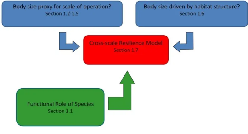
(24) Chapter 1: General Introduction particularly complex arena for scientists and managers aiming to quantify resilience. The predominance of studies using coral cover to indicate reef health, a coarse and ambiguous measure of condition, only enhances these difficulties (Hughes et al. 2010). To date there has been much discussion regarding drivers of resilience on reefs (Walker et al. 2006), presenting an array of potentially measurable indicators; however, empirical assessments are lacking (Carpenter, Westley & Turner 2005; Nyström et al. 2008). The cross-scale resilience model, which incorporates information on body size distributions and the spatial scales at which species interact with their environment and provide their function, has been suggested as one potential indicator of resilience (Peterson, Allen & Holling 1998; Allen, Gunderson & Johnson 2005). Overlap of function among species provides redundancy, if reduction or removal of a species that dominates a particular role results in an increased contribution by other species (Walker, Kinzig & Langridge 1999; McClanahan, Polunin & Done 2002). However, this redundancy is only valuable if members of a functional group respond differently to a disturbance; if they all respond in a similar manner the anticipated insurance value is lost (Elmqvist et al. 2003). The cross-scale resilience model proposes that where members of a functional group operate at different spatial scales, they will respond differently to a scale-specific disturbance, providing cross-scale redundancy (Peterson, Allen & Holling 1998). Thus, in quantifying how function is distributed across scales, the model provides a measure of resilience. To date the examination of functional distribution across scales and its implications for system resilience has been tested with respect to bird and invertebrate communities (e.g. Fischer et al. 2007; Angeler, Allen & Johnson 2013). However, this approach has not been applied in the context of coral reefs (Nyström et al. 2008). On reefs, the distribution of herbivore function across scales would provide an indication of the resilience of the process of herbivory, which could then be combined with other indicators such as the presence of a diverse and resistant coral assemblage (McClanahan et al. 2012), and connectivity among reefs (Nyström et al. 2008), to provide an overarching picture of the resilience of coral reefs. Application of the cross-scale resilience model on reefs now needs to be assessed to evaluate the usefulness of this approach. Implementation of the cross-scale resilience model is reliant on knowledge regarding the functional role of species, and is based on two main assumptions: (1) That body size is a useful proxy for the spatial scales over which species are delivering their ecosystem function. Therefore, the range of body sizes within a functional group indicates the range of scales over which a particular function is being provided; and (2) That habitat and resource availability at different spatial scales will influence the underlying body size distribution of associated animal 5.

(25) Chapter 1: General Introduction communities. Thus, to implement and evaluate the usefulness of the cross-scale resilience model on coral reefs, an essential first step is quantifying the spatial scales at which fish interact with the reef (Fig. 1-1).. Figure 1-1: Relationship between the cross-scale resilience model (red), required knowledge on the functional role of species (green), and the underlying assumptions of the model relating to the spatial ecology of reef fishes (blue).. 1.8. AIMS AND THESIS OUTLINE This study has two main aims, corresponding to the two parts of the thesis: Part 1 aims. to evaluate the spatial scales at which fish interact with the reef and provide their function; and Part 2 evaluates the application of the cross-scale resilience model in the context of coral reefs. These aims are addressed in seven separate studies focusing on distinct research questions: Part 1: Evaluate the spatial scales at which fish interact with coral reefs Chapter 2.. Is body size related to home range area in reef fish?. Chapter 3.. Is body size related to foraging movements in reef fish?. Chapter 4.. How are foraging movements influenced by habitat condition?. Chapter 5.. Do cross-scale distributions in habitat complexity drive fish body size distributions?. Part 2: Implement the cross-scale resilience model for coral reef fish Chapter 6.. What is the current state of knowledge regarding the cross-scale resilience model and its underlying conceptual framework, the discontinuity hypothesis?. 6.

(26) Chapter 1: General Introduction Chapter 7.. What body size distribution metrics are appropriate for evaluating the effect of habitat on coral reef fishes?. Chapter 8.. What is the relationship between cross-scale herbivore functional redundancy and reef benthic condition across and following a disturbance event?. The research questions are addressed in the seven studies outlined below, which correspond to the publications derived from this thesis.. Part 1 of the thesis tests the. assumptions underlying the cross-scale resilience model and is composed of four chapters: Chapter 2 is a quantitative review describing the allometric relationship between body length and home range area in reef fish, and exploring the effect of functional group and tracking method on this relationship. The review tests the premise that a species’ body size is indicative of the scale at which it operates. Chapter 3 investigates the allometry of foraging movements for herbivorous reef fish. Furthermore it assesses the range of scales over which different herbivore functional groups provide their role, and the potential effect of fishing on these patterns. Thus, this chapter provides an understanding of the spatial component of reef fish function. Chapter 4 explores the association between reef condition and foraging behaviour, exploring changes in foraging distances and areas on reefs with different disturbance and recovery histories.. This chapter provides an understanding of the dynamics of foraging. behaviour in response to habitat modifications. Chapter 5 quantifies patterns of cross-scale habitat complexity on reefs of different habitat types, and compares these patterns to body depth distributions of the associated fish community.. This investigation indicates the potential. influence of cross-scale habitat availability on the size distributions of allied taxa. Part 2 of the thesis is composed of three chapters: Chapter 6 is a literature review outlining the conceptual framework of the discontinuity hypothesis, which underpins the cross-scale resilience model. The review also explores applications of the discontinuity approach, including characterisation of scales within systems, identification of non-linear dynamics, and the cross-scale resilience model. Finally the review presents research gaps, highlighting the potential problems of using this approach in aquatic systems and for fish taxa. Chapter 7 builds on a key gap identified in Chapter 6, specifically it explores appropriate body size distribution metrics to use when evaluating the effect of habitat on associated taxa with either determinate or indeterminate growth. The results of this study inform the development of the analysis in Chapter 8. Chapter 8 draws together all the information from the earlier chapters, implementing the cross-scale resilience model in the context of coral reefs. Specifically it assesses the relationships between changing benthic condition and cross-scale redundancy within the associated herbivorous fish community. Thus, it provides an indication of the utility of the model as an indicator of reef resilience. 7.

(27) Chapter 1: General Introduction In characterising scale dependent function in reef fish, this thesis will provide a fundamental understanding of the spatial scales at which fish interact with their environment and perform functions critical to coral reef resilience. From a management perspective, this research will: 1) Identify the scales at which action is needed to support resilience; 2) Highlight areas that need protection to support existing resilience or counteract its erosion (Cumming et al. 2005); and 3) inform appropriate targeted actions such as gear-based management to allow recovery of certain body sizes and thus support key functional groups operating at certain spatial scales.. 8.

No results found