This is a repository copy of
Constrained consensus for bargaining in dynamic coalitional
TU games.
.
White Rose Research Online URL for this paper:
http://eprints.whiterose.ac.uk/89720/
Version: Accepted Version
Proceedings Paper:
Nedic, A and Bauso, D (2011) Constrained consensus for bargaining in dynamic coalitional
TU games. In: CDC-ECE. 2011 50th IEEE Conference on Decision and Control and
European Control Conference (CDC-ECC), December 12-15, 2011, Orlando, FL, USA.
IEEE , 229 - 234. ISBN 978-1-61284-800-6
https://doi.org/10.1109/CDC.2011.6160508
[email protected] https://eprints.whiterose.ac.uk/ Reuse
Unless indicated otherwise, fulltext items are protected by copyright with all rights reserved. The copyright exception in section 29 of the Copyright, Designs and Patents Act 1988 allows the making of a single copy solely for the purpose of non-commercial research or private study within the limits of fair dealing. The publisher or other rights-holder may allow further reproduction and re-use of this version - refer to the White Rose Research Online record for this item. Where records identify the publisher as the copyright holder, users can verify any specific terms of use on the publisher’s website.
Takedown
If you consider content in White Rose Research Online to be in breach of UK law, please notify us by
Constrained Consensus for Bargaining in Dynamic Coalitional TU
Games
Angelia Nedi´c and Dario Bauso
Abstract— We consider a sequence of transferable utility (TU) games where, at each time, the characteristic function is a random vector with realizations restricted to some set of values. We assume that the players in the game interact only with their neighbors, where the neighbors may vary over time. The game differs from other ones in the literature on dynamic, stochastic or interval valued TU games as it combines dynamics of the game with an allocation protocol for the players that dynamically interact with each other. The protocol is an iterative and decentralized algorithm that offers a paradigmatic mathematical description of negotiation and bargaining processes. The main contributions of the paper are the definition of a robust (coalitional) TU game and the development of a distributed bargaining protocol. We prove the convergence with probability 1 of the bargaining protocol to a random allocation that lies in the core of the robust game under some mild conditions on the players’ communication graphs.
I. INTRODUCTION
Coalitional games with transferable utilities (TU) have been introduced by von Neumann and Morgenstern [24]. They have been used to model cooperation in supply chain or inventory management applications [6], [10], network flow applications [2] and in communication networks [20].
In this paper, we consider a sequence of coalitional TU games for a finite set of players. The game is played repeatedly over time, thus generating a sequence of time varying characteristic functions. We refer to such a repeated game as dynamic coalitional TU game. In this setting, a player can observe only the allocations of his neighbors, which may change in time. The model used in the current paper is motivated by applications in the context of network flow problems and multi-inventory control as illustrated in [3], [4].
We consider bargaining protocols assuming that each player i obeys rationality and efficiency by deciding on an allocation vector which satisfies the value constraints of all the coalitions that include player i. This set is termed
bounding set of player i. At every iteration, a player i
observes the allocations of some of his neighbors. This is modeled using a directed graph with the set of players as the vertex set and a time-varying edge set composed of directed links(i, j)whenever playeriobserves the allocation vector proposed by player j at time t. We refer to this directed
A. Nedi´c is with the Industrial and Enterprise Systems Engineering Department, University of Illinois at Urbana-Champaign, Urbana IL 61801, USA,[email protected]
D. Bauso is with Dipartimento di Ingegneria Chimica, Gestionale, In-formatica e Meccanica, Universit`a di Palermo, V.le delle Scienze, 90128 Palermo, ITALY,[email protected]
graph as players’neighbor-graph. Given a player’s neighbor-graph, each player i negotiates allocations by adjusting the allocations he received from his neighbors through weight assignments. As the balanced allocation may violate his rationality constraints (it lies outside playeri’s bounding set), the player selects a new allocation by projecting the balanced allocation on his bounding set. We propose such bargaining protocols for solving the robust TU game. We use some mild assumptions on the connectivity of the players’ neighbor-graph and the weights that the players use when balancing their own allocations with the neighbors’ allocations. Assum-ing that the core of the robust game is nonempty, we show that our bargaining protocol converges with probability 1 to a common (random) allocation in the core.
The work in this paper deviate from the stochastic frame-work provided in [9], [21], [22] in at least three aspects: i) the existence of a neighbor-graph, ii) the presence of multiple iterations in the bargaining process, iii) and the consideration of the robust game. Also, a new element with respect to previous work [8], [11], is that the values of the coalitions are realized exogenously and no relation is assumed between consecutive samples.
Dynamic robust TU games have been considered in [3] and [4] but for a continuous time setting in the former work and for a centralized allocation process in the latter one. Convergence of allocation processes is a main topic also in [5], [13]. The difference with our approach is that in [5], [13], rewards are allocated by a game designer repeatedly in a centralized manner. Convergence of bargaining processes has also been explored under dynamic coalition formation [1] for a different dynamic model, where players decide both on which coalition to address and what payoff to announce.
The work in this paper is also related to the literature on agreement among multiple agents, where an underlying communication graph for the agents and balancing weights have been used with some variations [23], [15] to reach an agreement on common decision variable, as well as in [16], [17], [19], [18] for distributed multi-agent optimization.
This paper is organized as follows. In Section II, we introduce the dynamic TU game, the robust game and the bargaining protocol for this game. We then give some preliminary results. In Section III, we prove the convergence of the bargaining protocol to a point in the core of the robust game with probability 1. In Section IV, we report some numerical simulations to illustrate our theoretical study, and we conclude in Section V.
also usexi
to denote the vector associated to playeri. For two vectorsxandy, we usex < y (x≤y) to denote xi < yi (xi ≤yi) for all coordinate indicesi. We letx′ denote
the transpose of a vector x, and kxk denote its Euclidean norm. An n×n matrix A is row-stochastic if the matrix has nonnegative entries aij andPnj=1aij = 1 for all i =
1, . . . , n. For a matrix A, we useaij or [A]ij to denote its ijth entry. A matrix A is doubly stochastic if both A and its transposeA′are row-stochastic. Given two setsU andS, we write U ⊂S to denote thatU is a proper subset ofS. We use|S|for the cardinality of a given finite set S.
We writePX[x]to denote the projection of a vectorxon
a set X, and we write dist(x, X) for the distance from x
toX, i.e., PX[x] = arg miny∈Xkx−yk anddist(x, X) = kx−PX[x]k, respectively. Given a setXand a scalarλ∈R,
the setλX is defined by λX ,{λx |x∈X}. Given two setsX, Y ⊆Rn, the set sumX+Y is defined byX+Y ,
{x+y | x ∈ X, y ∈ Y}. Given a set N of players and a function η : S 7→R defined for each nonempty coalition
S⊆N, we write< N, η >to denote the transferable utility (TU) game with the players’ set N and the characteristic functionη. We letηS be the valueη(S)of the characteristic
function η associated with a nonempty coalition S ⊆ N. Given a TU game < N, η >, we use C(η) to denote the core of the game,
C(η) =
( x
X
i∈N
xi=ηN, X
i∈S
xi≥ηS for allS⊂N )
,
whereS is always considered to be non-empty.
II. DYNAMICTU GAME ANDROBUSTGAME
In this section, we formulate a robust dynamic TU game and introduce a bargaining protocol that the players imple-ment to reach an agreeimple-ment on their allocations. We also provide some preliminary results for the protocol.
A. Problem Formulation and Bargaining Process
Consider a set of players N ={1, . . . , n} and the set of all possible (nonempty)coalitions S⊆N among them. Let
m= 2n−1be thenumber of possible coalitions. We assume
that time is discrete and uset= 0,1,2, . . .to index the time. We consider a dynamic TU game, denoted< N,{v(t)}>, where{v(t)}is a sequence of characteristic functions. In this game, the players are involved in a sequence of instantaneous TU games whereby, at each time t, the instantaneous TU game is < N, v(t) > with v(t) ∈ Rm for all t ≥ 0. Further, we letvS(t)denotethe value assigned to a nonempty
coalition S ⊆ N in the instantaneous game < N, v(t) >. Throughout the rest of the paper, we assume that S 6= ∅, i.e.,we do not consider empty coalitions.
In what follows, we deal with dynamic TU games where each characteristic function v(t) is a random vector with realizations restricted to some set of values. Specifically, we assume that the grand coalition valuevN(t)is deterministic
for everyt≥0, while the valuesvS(t)of the other coalitions S ⊂N have a common upper bound. These conditions are formally stated in the following assumption.
Assumption 1: There exists vmax ∈Rm
such that for all
t≥0,
vN(t) =vNmax,
vS(t)≤vSmax for all coalitionsS⊂N.
We refer to the game < N, vmax >as robust game. We assume that the robust game has a nonempty core.
Assumption 2: The coreC(vmax)is not empty.
An immediate consequence of Assumptions 1 and 2 is that the core C(v(t)) of the instantaneous game is always not empty. This follows from the fact thatC(vmax)⊆C(η)
for anyη satisfyingηN =vmaxN andηS ≤vmaxS for S⊂N,
and the assumption that the core C(vmax)is not empty.
We assume that each playeriisrational and efficient. This translates to each playeri∈Nchoosing his allocation vector within the set of allocations satisfying value constraints of all coalitions that include playeri. This set is referred to as thebounding set of playeri. For a generic game< N, η >, it is given by
Xi(η) =
x∈Rn|X j∈N
xj =ηN, X
j∈S
xj≥ηS
for allS⊂N s.t.i∈S}.
Note that eachXi(η) is polyhedral.
In what follows, we find it convenient to represent the bounding sets and the core in alternative equivalent forms. For each coalition S ⊆ N, let eS ∈ Rn be the incidence
vector forS, i.e., the vector with the coordinates given by
[eS]i=
1 ifi∈S, 0 else.
Then, the bounding sets and the core are given by
Xi(η) ={x∈Rn |eN′ x=ηN, e′Sx≥ηS (1)
for allS⊂N withi∈S},
C(η) ={x∈Rn|eN′ x=ηN, e′Sx≥ηS (2)
for allS ⊂N}.
Observe that the core C(η) of the game < N, η > is the intersection of the bounding setsXi(η)of the players, i.e.,
C(η) =∩n
i=1Xi(η). (3)
We now discuss the bargaining protocol where repeatedly over time each player i∈N proposes an allocation vector. The allocation vector proposed by player i at time t is denoted byxi(t)∈
Rn, where thejth componentxi j(t)
rep-resents the amount that playeriwould allocate to playerj. To simplify the notation in the dynamic game < N,{v(t)} >, we let Xi(t) denote the bounding set of player i for the
instantaneous game < N, v(t) >, i.e., for all i ∈ N and
t≥0,
Xi(t) ={x∈Rn |e′Nx=vN(t), e′Sx≥vS(t) (4)
Now, we focus on players interactions in time. We assume that each player may observe the allocations of a subset of the other players at any time, which are termed as theneighbors of the player. The players and their neighbors at timetcan be represented by a directed graph G(t) = (N,E(t)), with the vertex set N and the set E(t) of directed links. A link (i, j) ∈ E(t) exists if player j is a neighbor of player i
at time t. We always assume that (i, i) ∈ E(t) for all t, which is natural since every player i can always access its own allocation vector. We refer to graphG(t)as a neighbor-graph at timet. In the graph G(t), a playerj is a neighbor of playeri (i.e., (i, j)∈ E(t)) only if player i can observe the allocation vector of playerj at timet.
Given the players’ neighbor-graph G(t), each player i
negotiates allocations by averaging his allocation and his neighbors’ allocations. More precisely, at timet, the bargain-ing process for each playeriinvolves the player’s individual bounding setXi(t), its own allocationxi(t)and the observed
allocationsxj(t)
of some of his neighborsj. Formally, we let
Ni(t)be the set of neighbors of playeriat timet(including
himself), i.e.,
Ni(t) ={j ∈N |(i, j)∈ E(t)}.
With this notation, the bargaining process is given by:
xi(t+1) =PXi(t)
X
j∈Ni(t)
aij(t)xj(t)
∀i∈N, t≥0 (5)
where aij(t) ≥ 0 is a scalar weight that player i assigns
to the proposed allocation xj(t)
of player j and PXi(t)[·]
is the projection onto the player i bounding setXi(t). The
initial allocations xi(0), i ∈ N,
are selected randomly and independently of {v(t)}.
The bargaining in (5) can be written more compactly by introducing zero weights for playersj whose allocations are not available to player i at time t. Specifically by defining
aij(t) = 0for allj6∈ Ni(t)andt≥0, we have the following
equivalent representation of the bargaining protocol:
xi(t+ 1) =PXi(t)
n X
j=1
aij(t)xj(t)
∀i∈N, t≥0. (6)
Here,aij(t) = 0forj6∈ Ni(t)andaij(t)≥0forj∈ Ni(t).
We now discuss the specific assumptions on the weights
aij(t)and the players’ neighbor-graph that we will rely on.
We let A(t) be the weight matrix with entries aij(t). We
will use the following assumption for the weight matrices.
Assumption 3: Each matrixA(t)is doubly stochastic with positive diagonal, and there exists a scalarα >0 such that
aij(t)≥α whenever aij(t)>0.
In view of the construction of matrices A(t), we see that
aij(t)≥ α for j = i and perhaps for some players j that
are neighbors of player i. The requirement that the positive weights are uniformly bounded away from zero is imposed to ensure that the information from each player diffuses to his neighbors in the network persistently in time. The
requirement on the doubly stochasticity of the weights is used to ensure that in a long run each player has equal influence on the limiting allocation vector.
It is natural to expect that the connectivity of the players’ neighbor-graphs G(t) = (N,E(t)) impacts the bargaining process. At any time, the instantaneous graph G(t) need not be connected. However, for the proper behavior of the bargaining process, the union of the graphsG(t)over a period of time is assumed to be connected.
Assumption 4: There is an integer Q ≥ 1 such that the graphN,S(t+1)Q−1
τ=tQ E(τ)
is strongly connected for every
t≥0.
Assumptions 3 and 4 together guarantee that the players communicate sufficiently often to ensure that the information of each player is persistently diffused over the network in time to reach every other player. Under these assumptions, we will study the dynamic bargaining process in (6). We want to provide conditions under which the process converges to an allocation in the core of the robust game. Before this, we provide some preliminary results in the following section.
B. Preliminary Results
In this section we derive some preliminary results pertinent to the core of the robust game. We also provide some error bounds for polyhedral sets applicable to the players’ bounding sets Xi(t). We later use these results to establish
the convergence of the bargaining process in (6).
In our analysis we often use the following relation that holds for the projection operation on a closed convex set
X ⊆Rn: for any w∈Rn and any x∈X,
kPX[w]−xk2≤ kw−xk2− kPX[w]−wk2. (7)
This relation is known as a strictly non-expansive projection property (see [7], volume II, 12.1.13 Lemma, page 1120).
We next relate the distance dist(x, C(η)) from a pointx
to the coreC(η)with the distancesdist(x, Xi(η))fromxto
the bounding setsXi(η). To do so, we use the polyhedrality
of the bounding setsXi(η)and the coreC(η), as given in (1)
and (2) respectively, and a special relation for polyhedral sets. This special relation states that for a nonempty polyhedral setP ={x∈Rn |aℓ′x≤bℓ, ℓ= 1, . . . , r},there exists a
scalarc >0 such that
dist(x,P)≤c r X
ℓ=1
dist(x, Hℓ) for allx∈Rn, (8)
whereHℓ={x∈Rn |a′ℓx≤bℓ} and the scalarc depends
only on the vectorsaℓ, ℓ= 1, . . . , r. Relation (8) is known as
Hoffman bound, as it has been established by Hoffman [12] Aside from the Hoffman bound, in establishing the forth-coming Lemma 1, we also use the fact that the square distance from a pointxto a closed convex setX contained in an affine setH is given by
dist2(x, X) =kx−PH[x]k2+ dist2(PH[x], X). (9)
Lemma 1: Let< N, η >be a TU game with a nonempty coreC(η). Then, there is a constantµ >0 such that
dist2(x, C(η))≤µ n X
i=1
dist2(x, Xi(η)) for allx∈Rn,
where µ depends on the collection of vectors {e˜S | S ⊂ N, S 6=∅}, where each e˜S is the projection of eS on the
hyperplane H={x∈Rn|e′Nx=ηN}.
Proof: Since the hyperplaneH contains the coreC(η) (see (2)), by relation (9) we have for allx∈Rn,
dist2(x, C(η)) =kx−PH[x]k2+ dist2(PH[x], C(η)). (10)
The pointPH[x]and the core C(η)lie in the hyperplaneH
(ann−1-dimensional affine set). By applying the Hoffman bound relative to the affine setH (cf. Eq. (8)), we obtain
dist(PH[x], C(η))≤c X
S⊂N
dist(PH[x], H∩HS),
where HS = {x ∈ Rn | e′Sx ≥ ηS}, while the constant c depends on the collection {˜eS, S ⊂N} of projections of
vectorseS on the hyperplaneH forS⊂N. Thus, it follows
dist2(PH[x], C(η))≤c2 X
S⊂N
dist(PH[x], H∩HS) !2
≤c2(m−1) X
S⊂N
dist2(PH[x], H∩HS), (11)
wheremis the number of nonempty subsets ofN, and the last inequality follows by(Pℓ
j=1aj)2 ≤ℓP ℓ
j=1a2j, which
holds for any set of scalars {aj, j = 1, . . . , ℓ} withℓ ≥1.
From Eqs. (10) and (11), we obtain for allx∈Rn, dist2(x, C(η)) ≤ kx−PH[x]k2
+ c2(m−1) X
S⊂N
dist2(PH[x], H∩HS)
≤ c1
X
S⊂N
kx−PH[x]k2
+ dist2(PH[x], H∩HS)
,
wherec1 = max{1, c2(m−1)}. Since the setH is affine,
by Eq. (9) we havekx−PH[x]k2+ dist2(PH[x], H∩HS) =
dist2(x, H∩HS), implying that for all x∈Rn,
dist2(x, C(η))≤c1
X
S⊂N
dist2(x, H∩HS).
From the preceding relation, it follows for allx∈Rn,
dist2(x, C(η))≤c1
X
S⊂N
|S|dist2(x, H∩HS), (12)
where|S|is the cardinality of coalitionS. Note that
X
S⊂N
|S|dist2(x, H∩HS)
= X
S⊂N X
i∈S
dist2(x, H∩HS)
=
n X
i=1
X
{S⊂N|i∈S}
dist2(x, H∩HS)
. (13)
We also note that Xi(η)⊂H ∩HS for each S ⊂N with i∈S, which follows by the definition ofHSand relation (1).
For any two closed convex setsX, Y ⊆Rnsuch thatX⊂Y, we have dist(x, Y) ≤ dist(x, X) for any x ∈ Rn. Thus,
since Xi(η)⊂ H∩HS for each S withi ∈ S, it follows
that for allx∈Rn,
dist(x, H∩HS)≤dist(x, Xi(η)). (14)
By combining Eqs. (12)–(14) we obtain for allx∈Rn,
dist2(x, C(η)) ≤ c1
n X
i=1
X
{S⊂N|i∈S}
dist2(x, Xi(η))
= c1κ
n X
i=1
dist2(x, Xi(η)),
where κ is the number of coalitions S that contain player
i, which is the same number for every player (κ does not depend oni). The desired relation follows by lettingµ=c1κ,
and by recalling that c1 = max{1, c2(m−1)} and that c
depends on the projectionse˜S of vectorseS, S⊂N, on the
hyperplaneH.
Note that the scalar µ in Lemma 1 does not depend on the coalitions’ valuesηS forS6=N. It depends only on the
vectorseS,S⊆N, and the grand coalition valueηN.
As a direct consequence of Lemma 1, we have the following result for the instantaneous game < N, v(t) >
under the assumptions of Section II-A.
Lemma 2: Let Assumptions 1 and 2 hold. We then have for allx∈Rn and allt≥0,
dist2(x, C(v(t)))≤µ n X
i=1
dist2(x, Xi(t)),
whereC(v(t)) is the core of the game< N, v(t)>, Xi(t)
is the bounding set of player i, and µ is the constant from Lemma 1.
Proof: By Assumption 2, we have that the core
C(vmax) is nonempty. Furthermore, under Assumption 1, we haveC(vmax)⊆C(v(t))for allt≥0, implying that the coreC(v(t))is nonempty for allt≥0.
Under Assumption 1, each coreC(v(t))is defined by the same affine equality corresponding to the grand coalition value,e′Nx=vNmax. Moreover, each coreC(v(t))is defined
through the set of hyperplanes HS(t) ={x∈Rn | e′Sx≥ vS(t)}, S ⊂ N, which have time invariant normal vectors eS,S ⊆N. Thus, the result follows from Lemma 1.
III. CONVERGENCE TOCORE OFROBUSTGAME
In this section, we prove convergence of the bargaining process in (6) to a random allocation in the core of the robust game with probability 1. We find it convenient to re-write bargaining protocol (6) by isolating a linear and a non-linear term. The linear term is the vectorwi(t)defined as:
wi(t) =
n X
j=1
Note that wi(t)
is linear in players’ allocations xj(t). The
non-linear term is the error
ei(t) =PXi(t)[wi(t)]−wi(t). (16)
Using (15) and (16), we can rewrite protocol (6) as follows:
xi(t+1) =wi(t)+ei(t) for alli∈N andt≥0. (17)
Recall that the weights aij(t)≥0 are such that aij(t) = 0
for all j 6∈ Ni(t). Also, recall that A(t) is the matrix with
entriesaij(t), which defines the vectorswi(t)in (15).
In what follows we will show that, with probability 1, bargaining protocol (15)–(17) converges to the coreC(vmax)
of the robust game < N, vmax >, provided that v(t) =
vmax happens infinitely often in time with probability 1.
To establish this we use some auxiliary results, which we develop in the next two lemmas.
The following lemma provides a result on the sequences
xi(t)
and shows that the errorsei(t)
are diminishing.
Lemma 3: Let Assumptions 1 and 2 hold. Also, assume that each matrix A(t) is doubly stochastic. Then, for bar-gaining protocol (15)–(17), we have
(a) Pni=1kxi(t)−xk2 converges for all x∈C(vmax).
(b) P∞ t=0
Pn
j=1kei(t)k2 < ∞ and limt→∞kei(t)k = 0
for alli∈N.
Proof: Byxi(t+1) =P Xi(t)[w
i(t)]
and by strictly non-expansive property of the Euclidean projection on a closed convex setXi(t)(see (7)), we have for alli∈N,t≥0 and x∈Xi(t),
kxi(t+ 1)−xk2≤ kwi(t)−xk2− kei(t)k2. (18)
Under Assumptions 1 and 2, the core C(vmax) is
con-tained in the core C(v(t)) for all t ≥ 0, implying that
C(vmax) ⊆ C(v(t)) for all t ≥ 0. Furthermore, since
C(v(t)) =∩n
i=1Xi(t), it follows thatC(vmax)⊆Xi(t) for
all i ∈N andt ≥0. Therefore, relation (18) holds for all
x∈C(vmax). Thus, by summing the relations in (18) over
i∈N, we obtain for allt≥0 andx∈C(vmax),
n X
i=1
kxi(t+1)−xk2≤ n X
i=1
kwi(t)−xk2− n X
i=1
kei(t)k2. (19)
By the definition ofwi(t)in (15), using the stochasticity of A(t)and the convexity of the squared norm, we obtain
n X
i=1
kwi(t)−xk2=
n X
i=1
n X
j=1
aij(t)xj(t)−x
2
≤ n X
j=1
n X
i=1
aij(t) !
kxj(t)−xk2.
By the doubly stochasticity ofA(t), we havePn
i=1aij(t) =
1for everyj, implyingPn i=1kw
i(t)−xk2≤Pn i=1kx
i(t)− xk2. By substituting this relation in (19), we arrive at
n X
i=1
kxi(t+1)−xk2≤
n X
i=1
kxi(t)−xk2−
n X
i=1
kei(t)k2.
(20)
The preceding relation shows that the scalar sequence
{Pn i=1kx
i(t)−xk2} is non-increasing for any given x ∈
C(vmax). Therefore, the sequence must be convergent since
it is nonnegative. Moreover, by summing the relations in (20) overt= 0, . . . , sand then, lettings→ ∞, we obtain
∞ X
t=0
n X
i=1
kei(t)k2≤
n X
i=1
kxi(0)−xk2,
which implies thatlimt→∞ei(t) = 0for alli∈N.
In our next result, we will use the instantaneous average of players allocations, defined as follows:
y(t) = 1
n n X
j=1
xj(t) for allt≥0.
The result shows that the difference between the bargaining payoff vector xi(t) for any player i and the average y(t)
of these payoffs converges to 0 as time goes to infinity. The proof essentially uses the line of analysis that has been employed in [17], where the setsXi(t)are static, i.e., Xi(t) =Xi for allt. In addition, we also use the rate result
for doubly stochastic matrices, as established in [15].
Lemma 4: Let Assumptions 3 and 4 hold. Suppose that for the bargaining protocol (15)–(17) we have
lim
t→∞ke
i(t)k= 0
for alli∈N.
Then, for every player i∈N we have
lim
t→∞kx i(
t)−y(t)k= 0, lim
t→∞kw i(
t)−y(t)k= 0.
Proof: For any t≥s≥0, define matrices Φ(t, s) =A(t)A(t−1)· · ·A(s+ 1)A(s),
with Φ(t, t) = A(t). Using the matrices Φ(t, s) and the expression for xi(t) in (17), we relate xi(t) with xi(s) at
a times for0≤s≤t−1, as follows:
xi(t) =
n X
j=1
[Φ(t−1, s)]ijxj(s) (21)
+
t−1
X
r=s+1
n X
j=1
[Φ(t−1, r)]ijej(r−1)
+e i
(t−1).
Using the doubly stochasticity ofA(t),y(t) = 1nPn j=1x
j(t)
and relation (21), we obtain for allt≥s≥0,
y(t) = 1
n n X
j=1
xj(s) +1
n t X
r=s+1
n X
j=1
ej(r−1)
. (22)
By our assumption, we have limt→∞kei(t)k= 0 for all i.
Thus, for any ǫ > 0, there is an integer ˆs ≥ 0 such that
kei(t)k ≤ ǫ
and (22) withs= ˆs, we obtain for alliandt≥sˆ+ 1,
kxi(t)−y(t)k= n X j=1
[Φ(t−1,sˆ)]ij−
1
n
xj(ˆs)
+
t−1
X
r=ˆs+1
n X
j=1
[Φ(t−1, r)]ij−
1
n
ej(r−1)
+ ei(t−1)− 1 n
n X
j=1
ej(t−1)
≤ n X j=1
[Φ(t−1,sˆ)]ij−
1 n kx j(ˆ s)k
+
t−1
X
r=ˆs+1
n X
j=1
[Φ(t−1, r)]ij−
1 n ke j
(r−1)k
+ kei(t−1)k+1 n
n X
j=1
kej(t−1)k.
Sincekei(t)k ≤ǫ for allt≥ˆsand alli, it follows that
kxi(t)−y(t)k ≤ n X
j=1
[Φ(t−1,sˆ)]ij−
1 n kx j
(ˆs)k
+ǫ t−1
X
r=ˆs+1
n X
j=1
[Φ(t−1, r)]ij−
1
n + 2ǫ.
Under Assumptions 3 and 4, the following result holds for the matrices Φ(t, s), as shown in [14] (see there Corollary 1):
[Φ(
t, s)]ij−
1 n
≤1− α
4n2
⌈t−Qs+1⌉−2
for allt≥s≥0.
Substituting the preceding estimate in the estimate for
kxi(t)−y(t)k
, we obtain
kxi(t)−y(t)k ≤1− α
4n2
⌈t−Qsˆ⌉−2 n X
j=1
kxj(ˆs)k
+nǫ t−1
X
r=ˆs+1
1− α
4n2
⌈t−Qr⌉−2
+ 2ǫ.
Lettingt→ ∞, we see that
lim sup
t→∞ kx i(
t)−y(t)k ≤nǫ ∞ X
r=ˆs+1
1− α
4n2
⌈t−Qr⌉−2
+ 2ǫ.
Note that P∞
r=ˆs+1 1−
α
4n2
⌈t−r
Q ⌉−2 < ∞, which by the
arbitrary choice of ǫyields
lim
t→∞kx
i(t)−y(t)k= 0
for alli∈N .
Now, we focus on Pn i=1kw
i(t)−y(t)k
. Since wi(t) = Pn
j=1aij(t)xj(t)and sinceA(t)is stochastic, it follows n
X
i=1
kwi(t)−y(t)k ≤ n X i=1 n X j=1
aij(t)kxj(t)−y(t)k.
Exchanging the order of the summations over, and then using the doubly stochasticity ofA(t), we have
n X
i=1
kwi(t)−y(t)k ≤ n X j=1 n X i=1
aij(t) !
kxj(t)−y(t)k
=
n X
j=1
kxj(t)−y(t)k.
Since limt→∞kxj(t) − y(t)k = 0 for all j, we have Pn
i=1kwi(t)−y(t)k → 0, implying kwi(t)−y(t)k → 0
for alli.
So far, the polyhedrality of the sets Xi(t) has not been
used. We now combine all pieces together, namely Lemma 2 that exploits the polyhedrality of the bounding sets Xi(t),
Lemma 3 and Lemma 4. This brings us to the following convergence result for the robust game< N, vmax>.
Theorem 1: Let Assumptions 1–4 hold. Also, assume that Prob{v(t) =vmax i.o.}= 1,
where i.o. stands for infinitely often. Then, the players allocationsxi(t)
generated by bargaining protocol (15)–(17) converge with probability 1 to an allocation in the core
C(vmax), i.e., there is a random vectorx˜ ∈ C(vmax) such
that with probability 1,
lim
t→∞kx i(
t)−x˜k= 0 for alli∈N .
Proof: By Lemma 3, the sequence{Pn
i=1kxi(t)−xk2}
is convergent for everyx∈C(vmax)and the errorsei(t)
are diminishing for each player i, i.e., kei(t)k → 0. Then, by
Lemma 4 we havekxi(t)−y(t)k →0 for alli. Hence,
{ky(t)−xk}is convergent for everyx∈C(vmax). (23)
We want to show that{y(t)} is convergent and that its limit is in the coreC(vmax)with probability 1. For this, we note that sincexi(t+ 1)∈X
i(t), it holds for allt≥0, n
X
i=1
dist2(y(t+ 1), Xi(t))≤ n X
i=1
ky(t+ 1)−xi(t+ 1)k2.
The preceding relation andkxi(t)−y(t)k →0
for alli∈N
(cf. Lemma 4) imply
lim
t→∞ n X
i=1
dist2(y(t+ 1), Xi(t)) = 0.
By Assumptions 1 and 2, and Lemma 2 we have fort≥0,
dist2(y(t+ 1), C(v(t)))≤µ n X
i=1
dist2(y(t+ 1), Xi(t)).
By combining the preceding two relations we see that
lim
t→∞dist
2(
y(t+ 1), C(v(t))) = 0. (24)
By our assumption, we have that the event {v(t) =
vω(t) =vmaxholds infinitely often (for infinitely manyt’s).
Let{tk} be a sequence such that
vω(tk) =vmax for allk≥0.
All the variables corresponding to the realization {vω(t)}
are denoted by a subscriptω. By relation (23) the sequence
{yω(t)}is bounded, therefore{yω(tk)}is bounded. Without
loss of generality (by passing to a subsequence of {tk}
if necessary), we assume that {yω(tk)} converges to some
vectory˜ω, i.e.,
lim
k→∞yω(tk) = ˜yω.
Thus, the preceding two relations and Eq. (24) imply that ˜
yω ∈ C(vmax). Then, by relation (23), we have that {kyω(t)−y˜ωk}is convergent, from which we conclude that
˜
yω must be the unique accumulation point of the sequence {yω(t)}, i.e.,
lim
t→∞yω(t) = ˜yω, y˜ω∈C(v
max).
This and the assumption Prob{v(t) =vmax i.o.} = 1,
imply that the sequence{y(t)}converges with probability 1 to a random point y˜ ∈ C(vmax). Since by Lemma 4 we have kxi(t)−y(t)k → 0 for every i, it follows that the
sequences{xi(t)}, i= 1, . . . , n,converge with probability 1
to a common random point in the coreC(vmax). IV. NUMERICALILLUSTRATIONS
In this section, we report some numerical simulations. We consider a dynamic coalitional TU game with 3 players, so the number of possible nonempty coalitions is m= 7. The characteristic functions vS(t) are generated independently
with identical uniform distribution over an interval. Specifi-cally, at each timet, the valuev{1}(t)is chosen randomly in
the interval[4,7]with uniform probability independently of the other times. Similarly, the values v{2}(t) are generated
in the interval[0,3]. The grand coalition value is fixed to 10 at all times, and the other coalition values are 0.
We run 50 different Monte Carlo trajectories each one having 100 iterations. The number of iterations is chosen long enough to show the convergence of the protocols. All plots include the sampled average and sampled variance for the 50 different trajectories that were simulated. Each trajec-tory is generated by starting with the same initial allocations, which are given by x1(0) = [10 0 0]′, x2(0) = [0 10 0]′,
andx3(0) = [0 0 10]′. The sampled average is computed for
each timet= 1, . . . ,100, by fixing the timetand computing the average value of the 50 trajectory sample values for that time. The sampled variance is computed as the variance of the samples with respect to their sampled average.
v1
v2 v3
(a)
v1
v2 v3
(b)
v1
v2 v3
[image:8.612.328.534.605.708.2](c)
Fig. 1. Topology of players’ neighbor-graph at three distinct times
t= 0, 1 and 2.
Regarding the players’ neighbor-graphs, we assume that the graphs are deterministic but time-varying. The graphs for the times t = 0,1,2 are as follows: player 2 and 3 connected at time t = 0 (see Figure 1(a)), then player 3 and 1 connected at time t = 1 (Figure 1(b)), and finally player 1 and 2 connected at timet= 3 (Figure 1(c)). These graphs are then repeated consecutively in the same order. In this way, the players’ neighbor-graph is connected every 2 time units (Assumption 4 is satisfied withQ= 2).
The matricesA(0),A(1)andA(2)that we associate with these three graphs, are respectively given by:
1 0 0 0 1
2 1 2
0 1 2
1 2
,
1
2 0
1 2
0 1 0
1
2 0
1 2
,
1 2
1
2 0
1 2
1
2 0
0 0 1
.
These matrices are also repeated in the same order for the rest of the time. Thus, at any time t, the matrix A(t) is doubly stochastic, with positive diagonal, and every positive entry bounded below by 12, so Assumption 3 is satisfied with
α = 1
2. All simulations are carried out with MATLAB on
an Intel(R) Core(TM)2 Duo, CPU P8400 at 2.27 GHz and a 3GB of RAM. The run time of each simulation is around 90 seconds.
The characteristic function vmax for the robust game is obtained by considering the highest possible coalition values which results invmax = [7 3 0 0 0 0 10]′. The resulting core
of the robust game is given by
C(vmax) ={x∈R3: x1≥7, x2≥3, x3≥0,
x1+x2≥0, x1+x3≥0,
x2+x3≥0, x1+x2+x3= 10}.
We note that this core contains a single point, namely[7 3 0]′.
To ensure that v(t) = vmax infinitely often, as required by Theorem 1 for the convergence of the protocol, we adopt the following randomization mechanism. At each time
t= 1, . . . ,100, we flip a coin and if the outcome is “head” (probability 1/2), the coalitions’ values v{1}(t) and v{2}(t)
are extracted from the intervals[4,7]and[0,3], respectively, with uniform probability independently of the other times. If the outcome of the coin flip is “tail”, then we assume that the robust game realizes and takev(t) =vmax.
We next present the results obtained by the Monte Carlo runs for the bargaining protocol in (15)–(17). An illustration of a typical run with the allocations generated in periods
t= 0,1,2,3 is shown below:
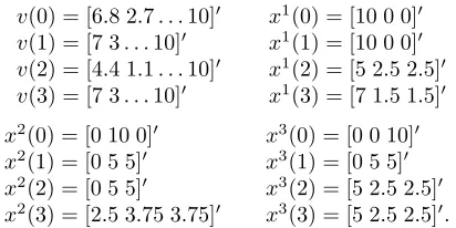
v(0) = [6.8 2.7. . .10]′
v(1) = [7 3. . .10]′
v(2) = [4.4 1.1. . .10]′
v(3) = [7 3. . .10]′
x1(0) = [10 0 0]′ x1(1) = [10 0 0]′ x1(2) = [5 2.5 2.5]′ x1(3) = [7 1.5 1.5]′ x2(0) = [0 10 0]′
x2(1) = [0 5 5]′ x2(2) = [0 5 5]′ x2(3) = [2.5 3.75 3.75]′
x3(0) = [0 0 10]′
x3(1) = [0 5 5]′ x3(2) = [5 2.5 2.5]′ x3(3) = [5 2.5 2.5]′.
Fig. 2. Plots of the sampled average (left) and variance (right) of players’ allocationsxi
(t),i= 1,2,3generated by bargaining protocol (15)–(17). Sampled averages of the allocationsxi
(t)converge to the same point˜x= [7 3 0]′∈C(vmax
), while sampled variances go rapidly to zero.
timet= 1, bargaining involves player 2 and 3 who update the allocations respectively asx2(1) = [0 5 5]′ andx3(1) =
[0 5 5]′. These allocations are feasible for their bounding sets so the projections on these sets are not performed. At time
t = 2, the bargaining involves player 1 and 3 who update their allocations, respectively, as x1(2) = [5 2.5 2.5]′ and x3(2) = [5 2.5 2.5]′. Again, these allocations are feasible
for their bounding sets and the projections are not performed. Finally, at timet= 3, the bargaining involves player 1 and 2 who update their allocations resulting inx1(3) = [7 1.5 1.5]′
andx2(3) = [2.5 3.75 3.75]′. Notice that x1(3) is obtained
after player 1 projects onto his bounding set.
In Figure 2 we report our simulation results for the average of the sample trajectories obtained by Monte Carlo runs. We show the sampled average and variance of the allocations
xi(t), i = 1,2,3
per iteration t. In accordance with the convergence result of Theorem 1, the sampled averages of the players’ allocations xi(t)
converge to the same point, namelyx= [7 3 0]′ which is in the core of the robust game
C(vmax).
V. CONCLUSIONS
This article deals with dynamics and robustness within the framework of coalitional TU games. The novelty of the work lies in the design of a decentralized allocation process defined over a communication graph of players. The key properties that distinguish this work from the existing work on dynamic games are: (1) the introduction of a time-varying communication graph; and (2) the distributed bargaining protocol for players’ allocations updates subject to local information exchange with neighboring players.
REFERENCES
[1] T. Arnold and U. Schwalbe. Dynamic coalition formation and the core. Journal of Economic Behavior and Organization, 49:363–380, 2002.
[2] D. Bauso, F. Blanchini, and R. Pesenti. Optimization of long-run average-flow cost in networks with time-varying unknown demand.
IEEE Transactions on Automatic Control, 55(1):20–31, 2010.
[3] D. Bauso and P. V. Reddy. Robust allocation rules in dynamical cooperative TU games. Proc. of the 49th Conference on Decision and Control, 2010.
[4] D. Bauso and J. Timmer. Robust dynamic cooperative games.
International Journal of Game Theory, 38(1):23–36, 2009.
[5] J.C. Cesco. A convergent transfer scheme to the core of a TU-game.
Revista de Matem´aticas Aplicadas, 19(1–2):23–35, 1998.
[6] J. Drechsel.Cooperative Lot Sizing Games in Supply Chains. Springer-Verlag. Series: Lecture Notes in Economics and Mathematical Sys-tems, Berlin, Germany, 1 edition, 2010.
[7] F. Facchinei and J-S. Pang.Finite-dimensional variational inequalities and complementarity problems, volume I-II. Springer-Verlag, New York, 2003.
[8] J.A. Filar and L.A. Petrosjan. Dynamic cooperative games. Interna-tional Game Theory Review, 2(1):47–65, 2000.
[9] D. Granot. Cooperative games in stochastic characteristic function form. Management Sci., 23:621–630, 1977.
[10] B.C. Hartman, M. Dror, and M. Shaked. Cores of inventory central-ization games. Games and Economic Behavior, 31:26–49, 2000. [11] A. Haurie. On some properties of the characteristic function and
the core of a multistage game of coalitions. IEEE Transactions on Automatic Control, 20(2):238–241, 1975.
[12] A.J. Hoffman. On approximate solutions of systems of linear in-equalities. Journal of Research of the National Bureau of Standards, 49:263–265, 1952.
[13] E. Lehrer. Allocation processes in cooperative games. International Journal of Game Theory, 31:341–351, 2002.
[14] A. Nedi´c, A. Olshevsky, A. Ozdaglar, and J.N. Tsitsiklis. Distributed subgradient methods and quantization effects. Proc. of the 47th CDC Conference, 54(11):4177–4184, 2008.
[15] A. Nedi´c, A. Olshevsky, A. Ozdaglar, and J.N. Tsitsiklis. On distributed averaging algorithms and quantization effects. IEEE Transactions on Automatic Control, 54(11):2506–2517, 2009. [16] A. Nedi´c and A. Ozdaglar. Distributed subgradient methods for
multi-agent optimization. IEEE Transactions on Automatic Control, 54(1):48–61, 2009.
[17] A. Nedi´c, A. Ozdaglar, and P.A. Parrilo. Constrained consensus and optimization in multi-agent networks.IEEE Transactions on Automatic Control, 55(4):922–938, 2010.
[18] S. Sundhar Ram, A. Nedi´c, and V.V. Veeravalli. Incremental stochastic subgradient algorithms for convex optimization. SIAM Journal on Optimization, 20(2):691–717, 2009.
[19] S. Sundhar Ram, A. Nedi´c, and V.V. Veeravalli. Distributed stochastic subgradient algorithm for convex optimization. Journal of Optimiza-tion Theory and ApplicaOptimiza-tions, 147(3):516–545, 2010.
[20] W. Saad, Z. Han, M. Debbah, A. Hj¨orungnes, and T. Bas¸ar. Coalitional game theory for communication networks. IEEE Signal Processing Magazine, Special Issue on Game Theory, 26(5):77–97, 2009. [21] J. Suijs and P. Borm. Stochastic cooperative games: Superadditivity,
convexity, and certainty equivalents.Games and Economic Behavior, 27(2):331–345, 1999.
[22] J. Timmer, P. Borm, and S. Tijs. On three shapley-like solutions for cooperative games with random payoffs. International Journal of Game Theory, 32:595–613, 2003.
[23] J.N. Tsitsiklis.Problems in Decentralized Decision Making and Com-putation. PhD thesis, Dept. of Electrical Engineering and Computer Science, MIT, 1984.
![Fig. 2.Plots of the sampled average (left) and variance (right) of players’[7 3 0]allocations xi(t), i = 1, 2, 3 generated by bargaining protocol (15)–(17).Sampled averages of the allocations xi(t) converge to the same point ˜x =′ ∈ C(vmax), while sampled variances go rapidly to zero.](https://thumb-us.123doks.com/thumbv2/123dok_us/7997131.207639/9.612.56.328.51.202/allocations-generated-bargaining-protocol-averages-allocations-converge-variances.webp)
