This is a repository copy of Field Studies and Modeling Exploring Mean and Maximum
Water Age Association to Water Quality in a Drinking Water Distribution Network.
White Rose Research Online URL for this paper:
http://eprints.whiterose.ac.uk/84623/
Version: Accepted Version
Article:
Machell, J. and Boxall, J. (2011) Field Studies and Modeling Exploring Mean and
Maximum Water Age Association to Water Quality in a Drinking Water Distribution
Network. Journal of Water Resources Planning and Management, 138 (6). 624 - 638.
ISSN 0733-9496
https://doi.org/10.1061/(ASCE)WR.1943-5452.0000220
[email protected] https://eprints.whiterose.ac.uk/ Reuse
Unless indicated otherwise, fulltext items are protected by copyright with all rights reserved. The copyright exception in section 29 of the Copyright, Designs and Patents Act 1988 allows the making of a single copy solely for the purpose of non-commercial research or private study within the limits of fair dealing. The publisher or other rights-holder may allow further reproduction and re-use of this version - refer to the White Rose Research Online record for this item. Where records identify the publisher as the copyright holder, users can verify any specific terms of use on the publisher’s website.
Takedown
If you consider content in White Rose Research Online to be in breach of UK law, please notify us by
- 1 -
Field Studies and Modeling Exploring Mean and Maximum Water Age Association to Water Quality in a Drinking Water Distribution Network
John Machell 1 and Joby Boxall 2
Abstract: This paper presents the findings of an investigation into predicted / modeled water age and the
associated quality characteristics within a UK drinking water distribution network to determine if there was a
discernable link. Aquis (7-Technologies A/S, Denmark) hydraulic and water quality software were used to
identify water volumes of different ages, generated by localized demand patterns in pipes in close proximity to
one another. The pipe network studied was small spatially, of a single material, having a consistent demand due
to serving predominately light industry, but with interesting hydraulic patterns involving loops and mixing of
water volumes, and some long retention times. Field work was undertaken to obtain water quality samples from
five network locations identified as containing a broad range of calculated water age. The samples were
analyzed for standard regulated parameters by a UKAS (NAMAS) accredited water laboratory in line with UK
water industry standard quality assurance practice. The water sample analytical results were examined to see
how a number of physical, chemical and bacteriological parameters related to the calculated water age at each
sample point, heterotrophic plate counts being used as the indicator of general bacteriological water quality.
Limited association between the calculated water mean age and quality parameters was observed. Further
investigations, taking into account mixing of different aged water volumes and the maximum age contributions
to the mean age at each sample location, produced some association. The work demonstrated that mean age is
not a sufficient guide to general water quality in this small network area. Mixing effects, and maximum age
volume contributions, need to be taken into account if a more comprehensive understanding of water quality is
to be obtained.
CE Database subject headings: Drinking water, water quality, distribution networks, modeling, age of water,
mean age, maximum age, simulation
1
Research Fellow, Pennine Water Group, Civil and Structural Engineering, University of Sheffield, Mappin
Street, Sheffield S1 3JD, United Kingdom
2
Professor of Water Infrastructure Engineering, Civil and Structural Engineering, University of Sheffield,
- 2 -
INTRODUCTION
Most water distribution networks across the developed world regularly suffer a low, but persistent, number of
failed water quality samples. Despite extensive conventional investigation and expansive intervention, it was
reported that for many cases in the United Kingdom the cause of these failures, especially bacteriological
failures, could not be satisfactorily explained; UKWIR (2006). This is perhaps not surprising considering that
drinking water distribution networks are complex dynamic systems, comprised of a number of different
materials, introduced over several decades, with long residence times; in the order of days. The pipe material
condition within these networks varies widely because of the effects of historic water quality, corrosion,
material accumulations, temperature differentials, disinfection regimes and biological colonization by a variety
of micro-organisms. In recent years, ever tighter regulation has prompted water companies and researchers to
investigate aspects of water quality that has highlighted the complexity of interactions between hydraulic (flow
velocity, pressure); physical (temperature, color, turbidity, taste and odor); chemical (chlorine, tri-halomethanes,
metals); microbial (heterotrophs, coliforms, Ecoli); and biological (parasitic protozoa, helminths) within
distribution networks. In order to understand, and eventually better control the quality of water passing through
pipe networks, efforts to evaluate and model some of these interactions have been made with some success.
Despite the associated knowledge base, in our opinion, it is not yet possible to model most water quality
parameters without a great deal of experimental effort and field work because knowledge about reaction kinetic
constants, pipe wall and bulk water coefficients, nutrient requirements and other key model data is not
sufficiently developed to be readily applicable. The work presented here investigates one possible practicable
method that might help to explain the reasons for, and network areas likely to be susceptible to, these water
quality sample failures; especially the sporadic bacteriological failures. This paper presents the findings from a
study of the effect of mixing different water ages at nodes in a small network area of looped pipes on water
quality. The mean water age, and maximum age volume contribution to the mean water age were calculated
using hydraulic and water quality software at five locations from which water quality samples were taken. The
calculated water age and water quality sample analytical results were evaluated to determine if there was a
discernable link.
- 3 -
Water quality changes within a distribution network originate from hydraulic regimes and numerous physical,
chemical and biological reactions and interactions between the various materials that comprise distribution
assets and the composition of the bulk water volume. The reactions associated with these changes are mostly
kinetic in nature and will therefore be governed by time. Authors have frequently alluded that the longer
drinking water is in contact with the materials of a distribution network the higher the propensity for water
quality to be affected in some way. Many of these works are summarized in the AWWA report entitled “The
Effects of Water Age on Distribution System Water Quality” (AWWA 2002); and it is stated that water age is a
major factor in water quality deterioration. Other works suggest that it may be possible to use water age as a
surrogate indicator of water quality in general. Water age is not a definitive or defined parameter, but can
theoretically be associated with many of the physical, chemical and biological parameters used to quantify and
regulate water quality.
Physical
Increasing water temperature leads to increased bacteriological activity, may initiate new reactions, increase the
rates of existing reactions, and will push the reaction equilibrium towards by-product formation; for example,
the formation of trihalomethanes (THMs) from chlorine and precursor materials, such as organic color (Reilly
and Kippin 1983, Hass et al. 1984, Chung et al. 2003, Toroz and Uyak 2005). LeChevallier et al. (1996) showed
that water temperature, flow velocity (variations) and residence time have an impact on microbial activity and
that biological activity increases about 100% when temperature increases by 10 ºC and a temperature of 15 ºC
was critical for coliform growth.
Chemical
Older water was shown by Burlingame (1995) to be more corrosive to iron pipes when compared to that caused
by relatively young water, and that where phosphate compounds were used for corrosion control, their efficacy
could be diminished with time because hydrolyzing reactions reduce the impact of the phosphates on the
discoloration producing corrosion mechanisms. Mutoti et al. (2007) demonstrated that the release of iron in
distribution networks was a function of the water chemistry and the hydraulic flows, and hence water age,
within the network. Rossman et al. (1994) and Wu et al. (2005) highlighted that older water may have little or
no residual disinfectant due to substance decay and reactions with network materials with the result that the
- 4 -
could give rise to unpleasant tastes and odors. Srinivas et al. (2008) evaluated the effects of chlorine and
residence time on the presence of culturable bacteria in biofilms compared to that in bulk water, and found that
bulk water bacteria may dominate in portions of a distribution system that have low chlorine residual.
Biological
Biological issues in distribution networks include bacteriological regrowth (Camper 2004, Regan et al. 2003)
biofilm formation (Emtiazi et al. 2004, Berry et al. 2006) and microbial corrosion (Beech and Sunner 2004).
Factors influencing bacteriological re-growth include temperature (Szewzyk et al. 2000); water residence time
(water age) (LeChevallier 1990); concentration of organic compounds (Percival and Walker 1999); residual
disinfection concentration (Niquette et al. 2001); and distribution system materials (Keinänen-Toivola et al.
2004). Kirmeyer et al. (2000) showed that operational practices impact on slow growing organisms, such as
nitrifying bacteria. (Speh et al. 1976, LeChevallier et al. 1987, Prévost et al. 1997) showed that locations with
long residence time, such as the peripheral parts of the distribution system and service reservoirs, are vulnerable
to bacteriological re-growth because of decreased disinfectant residual, the transportation of sediments, and
increase in water temperature.
Heterotrophic plate counts (HPC)
The World Health Organisation explain that undertaking plate counts as part of a suite of analyses when
responding to claims of ill health is the most widespread use of HPC analysis, with most water suppliers doing
counts at both 37 °C and 22 °C, but a few only at 37 °C. The rationale is that plate counts may indicate a
significant event within the distribution network, not that HPC bacteria may be related to ill health. Plate counts
are also widely used when investigating complaints of poor taste or odor, as changes in HPC populations may
indicate proliferation of biofilms, which can be associated with microbial mediated generation of some
organoleptic compounds (Standing Committee of Analysts 1998). Operationally plate counts are also commonly
used as part of acceptance criteria for new mains prior to being put into supply and in assessing water quality
following mains rehabilitation work. The use of counts of heterotrophic bacteria has, therefore, a long history in
the United Kingdom. The count at 22 °C has been used as a general indicator of water quality since 1885. The
count at 37 °C was originally introduced with the belief that it could indicate potential faecal contamination, and
although this has now been disregarded, it is still used for operational management in the United Kingdom
- 5 -
faecal contamination, but are of use as indicators of general microbial quality. This acknowledges that some
coliform bacteria may be part of the natural bacterial flora in water and proliferate in biofilms. Coliforms are
also considered useful for monitoring the effectiveness of water treatment processes and the disinfection of new
or rehabilitated mains (Standing Committee of Analysts 2002). HPC has no health effects, it is indicative of
network cleanliness or the relative amount of contamination; it is generally accepted that the lower the
concentration of bacteria in drinking water, the better the water system is being maintained. Therefore 2, 3, 5
and 7-day HPC were used as an indicator of water quality “change”.
Water age modeling
There are a number of hydraulic and quality simulation software packages that can calculate water age;
EPANET (USEPA), Piccolo (Allied Power), SynerGEE Water (Advantica), InfoWorks WS
(Wallingfordsoftware), Aquis (7-Technologies A/S). A thorough understanding of mean water age profiles
across a network can facilitate the opportunity to introduce design options and operational strategies that are
aimed at reducing mean water age and hence microbial contamination (Water Science and Technology Board
2005). Prasad and Walters (2006) used an evolutionary computational model to establish the optimum minimum
water age in a given network. However, whilst there is a lot of anecdotal and idealized data concerning the
association of water age and water quality, this relationship has never really been demonstrated in a live
distribution network. Modeling mean water age is a good method for obtaining an overview of the age
distribution across a water distribution network. However, most mean age models calculate a flow weighted
average value at nodes as if they were different concentrations of the same chemical; but it is not correct to treat
water age in this way. Mixing two different water age volumes produces a single volume comprised of two
different age components, and the mixture does not necessarily have the characteristics of either of the original
volumes, or the average of the two. The mathematics applied in this manner causes small, older, water age
components to be disguised, and gives no indication of their origin. Machell et al. (2009) presented a water
quality model that enhanced aspects of current methods. The modified approach predicted water age
distributions by allocating water volumes to “age bins” and calculated the percentage of different volumes
mixing at nodes thereby keeping track of the different age components being mixed. The method also monitored
the maximum age of water within all pipes in the network. This functionality is available in the Aquis
(7-Technologies A/S) software and was used here to determine the maximum age component in a small area of a
- 6 -
From the evidence in the literature it seems clear that the longer water is in contact with the fabric of the
distribution network, the higher the propensity for different physical, chemical, and biological parameters, and
overall water quality, to deteriorate, and that this might be reflected using simulated water age.
AIMS AND OBJECTIVES
The aim of this work was to investigate whether water age simulations can be a useful surrogate for water
quality. This was undertaken through field studies in a small localized area of a distribution network comprised
of a small number of pipes of the same material and size, exhibiting interesting hydraulic patterns due to a
looped layout. Software predictions for both mean age and maximum age contribution to the mean age of water
were explored.
METHODOLOGY
Water age is a potential surrogate for water quality and this work investigated the distribution of water ages, not
absolute values. Water age was therefore allocated to “age bins”, and the water quality associated with each age
bin was compared. The objective was to demonstrate whether calculated water age could be used as a surrogate
indicator of overall water quality by trying to better understand the effect of water mixing and maximum age
contribution to the mixed volumes. This understanding might then be used to determine why and where poor
water quality might be manifest in a distribution network. Aquis (7-Technologies A/S) hydraulic and water
quality modeling software was used to calculate mean water age in a water supply network. A hydraulic model
consistent with currently UK build practice was used, pressure calibrated to data from a 1 week intensive survey
to an accuracy of +/-0.5mwc. The simulation results generated were used to identify a small localized area of the
network containing water volumes of different ages. A geographically small area with pipes of a single material,
with a consistent demand due to light industry was identified. Five sample points were set up where interesting
hydraulic patterns were predicted to be generated by pipe loops and mixing of water volumes, and where some
long retention times were exhibited; providing a broad range of water age and potential for changes in water
quality. Field work was then undertaken to obtain water quality samples over a five day period. The water
sample analytical results were examined to see how a number of physical, chemical and bacteriological
parameters related to the calculated water age at each sample point.
- 7 -
The study area, dominated by light industry, was selected for its hydraulic complexity (looped configuration),
but physical simplicity (pipe material and size). The pipe network was high pressure polyethylene (HPPE),
comprised of sections of relatively short pipe lengths of consistent diameter, which were nested in two loops,
providing an interesting range of ageing and mixing effects. The area took supplies from two different water
treatment plants blended prior to entry to the distribution network. One plant treated upland reservoir water
using ferric sulfate as the primary coagulant, and the second plant had two separate treatment trains; one for
upland reservoir water, and one for river water; both used aluminum sulfate based treatment trains. The Aquis
models were used to calculate the mean age of water volumes within each pipe in the study network area. The
outlet of the service reservoir supplying the network was allocated an age of zero hours. Cyclic extended period
model simulations were run to ensure stable water age values were calculated for each pipe. It was evident from
results that stable, repeatable age values were obtained; and this was the case for all the sites; Figure 1. The
numeric mean water age values are summarized in Table 1, these are the 24 hour average values for day 19 of
simulation. Calculated water mean age was then plotted against a street map background to determine where
stand-pipes could be fitted to take water quality samples from the water age volumes of interest. Five water
quality sampling locations were identified; Figure 2 shows their location on a map background that also shows
the topography of the pipes and the range of mean water age within them. Sample point 1 was located on the
inlet main supplying the area immediately prior to the localized looped part of the network; effectively acting as
a common inlet and reference point for water quality sample analysis. Sample point 2 was on the first main
supplied inside the looped part of the localized area. Sample points 3 and 4 were on 2 different pipe loops and
sample point 5 was on a leg from the looped pipes. Unfortunately, fire hydrants coincident with the water
volumes of interest were only available at 3 of the potential sampling locations SP1, SP4 and SP5, and the one
at SP5 was not ideally located but deemed usable in the absence of any alternative. Alternative solutions for the
other 2 mains were found in the form of a flow meter chamber at the inlet to industrial premises for SP3, and a
sample tap in an in-line meter pit at SP2. The tap at SP2 was used without modification and the flow meter at
SP3 was removed, and a hydrant and stand pipe installed. The stand pipes used comprised a standard UK
hydrant cap, approximately 1m of 13mm diameter pipe, and a regulation sample tap.
Water Quality Sampling
The previously installed sample tap in the meter chamber at SP2 was checked and prepared simply by flushing,
- 8 -
were prepared by thorough cleaning. Hydrant bowls were doused with disinfectant, and the stand pipes were
attached to the fire hydrants and disinfected in situ with the highly chlorinated water from the hydrant bowls by
opening the hydrant until chlorinated water had completely filled the stand pipe and was spilling out. Following
24-hour disinfection, the fire hydrants were slowly opened to gently flush the highly chlorinated water out of the
apparatus. During this preparatory work, Aquis was used to simulate diurnal flow patterns in the pipes chosen
for the sampling program. The modeled diurnal pipe flow results were used to determine an appropriate flow
rate through each stand pipe during the water quality sampling period. Flow rates were set to ensure that normal
flow patterns for each pipe in the network were not disrupted / exceeded during the sampling exercise and hence
minimal impact on water age. Water quality samples were collected from all 5 sample points at 6am, 9am and
12 noon, each day for 5 days; producing 75 samples in total. Each sample point was run for 2 minutes prior to
samples being collected. It was decided that repeated sampling per day was necessary to yield representative
daily average values. 6am, 9am and 12 noon provided samples representative of overnight, peak demand and
daytime operation respectively. This was intended to overcoming any variability due to the influence of daily
patterns in hydraulic conditions. Repeating this sampling for 5 consecutive weekdays was deemed the minimum
necessary to provide indication of possible water quality trends. Sampling weekdays only, minimized possible
effects of different demand patterns over the weekend. The 75 sample total that this strategy generated
represented a significant program of work and additional sampling was not practicable. The results from the
first and second day 6 am samples revealed elevated iron levels (after 18 hour standing). Since the pipes were
PVC in this area and there had been no excessive hydraulic disturbance, this was thought to be due to iron from
the hydrant bowls or stand pipes. 2 min and 5 min flushed samples were therefore taken for the early morning
(6am) sample round during the last 3 days of sampling. It was determined from these that there was a
measurable change in water quality caused by the stand pipes, therefore only the 5 min flushed samples have
been used in the analysis, and the iron results for days 1 and 2 were discarded.
Water Quality Analysis
Water quality in the UK is generally of a very high standard, and observing measurable deterioration in any
quality parameter within a stable distribution network is difficult. Significant change in water quality within a
network tends only to occur, for example, during events such as burst mains where the resultant change in flow
velocity disturbs corrosion products or other material accumulations. Therefore it was necessary to monitor for
- 9 -
parameters monitored were chosen because they represented physical, chemical and biological measures that are
indicative of general water quality. 2, 3, 5 and 7-day HPC were chosen as the focus of the bacteriological
analysis because coliforms and e-coli are rarely found in potable water in UK networks, and because they
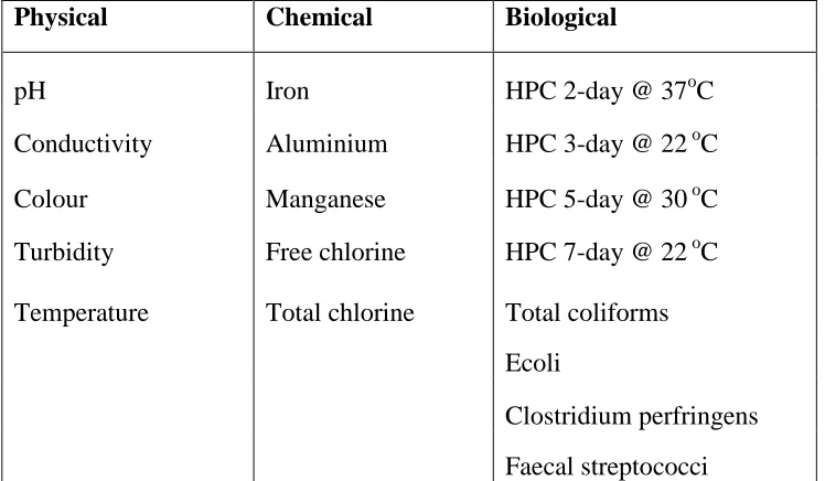
represented the best standard measure available to the project. The samples were analyzed for the water quality
parameters shown in Table 2 by a UKAS (NAMAS) accredited water analysis laboratory in line with UK
standard quality assurance practice.
Physicals
pH, conductivity, color, turbidity and temperature were used to represent the physical parameters. No change
was expected for pH, conductivity was potentially an indicator of change in dissolved ionic species, color and
turbidity being indicative of iron corrosion and / or bacteriological activity or sloughing of biological material
from biofilms. Turbidity can also be generated when hydraulic events disturb accumulated particulate material.
Metals
Iron, aluminum and manganese are the most routinely monitored metals reflecting water treatment process
failures, corrosion of metallic network components and hydraulic disturbance of material accumulations and
corrosion products. These parameters are often linked to aesthetic water quality problems; the most severe being
where the network is mostly old cast iron mains. Effective water treatment reduces iron and manganese, but past
treatment inadequacies will have caused iron and manganese to accumulate, particularly in low flow velocity
areas of the network. When these materials are disturbed, they may cause black, brown or orange discoloration
which may, in turn, result in failed regulatory turbidity samples. High iron or manganese residuals are
unacceptable because they can cause the bulk water to appear turbid, give rise to astringent or bitter tastes, and
the deposits are unsightly and may stain water fittings, and fast washing machine spin speeds may cause brown
or black staining on washing due to oxidative effects.
Chlorine
Chlorine is the most widely used disinfectant in the UK and monitoring free and total chlorine is useful to
measure the potential for bacteriological re-growth and proliferation. The difference between free and total
residual values is indicative of the presence of pollutants such as ammonia, or oxidizable organic material; and
- 10 -
an indicator of the health of the water within the network and its potential to prevent the proliferation of
microbial organisms.
Biological
Bacteriological analysis parameters included total coliforms, Ecoli, faecal streptococci, clostridium perfringens
and heterotrophic plate counts. Coliforms consist of a related group of bacteria species from human and animal
waste (faecal origin), and from environmental sources (vegetative origin). Coliforms are used as indicator
organisms because their presence is indicative of contamination. Total coliforms indicate the presence of both
vegetative and faecal contamination. Ecoli is found in the intestinal tract of warm-blooded animals and is
indicative of pollution from human or animal waste. Faecal streptococci can provide evidence of recent faecal
contamination. Clostridium perfringens is a useful indicator of either intermittent or historical faecal
contamination of a groundwater source, or surface water filtration plant performance. The detection of either
organism should trigger investigation because pollution caused by fecal contamination presents the potential for
consumers to contract pathogenic diseases. 2, 3, 5 and 7-day Heterotrophic Plate Counts (HPC) were chosen as
the primary indicator of water quality “change”. Colony counts serve as a relatively easy way to measure
estimated numbers of bacteria that have the potential for increased contamination. The most widely applied
routine test in most of the UK is 2-day and 3-day HPC. However, when investigational sampling is required (in
response to an illness complaint for example) 5-day and 7-day counts are also done as these provide extra
information about slower growing organisms as well as the 2-day and 3-day counts information. More advanced
water quality analysis were not considered, as the objective here was to discern if water age modeling was a
useful surrogate to currently applied and regulated water quality parameters.
RESULTS
Mean Water age
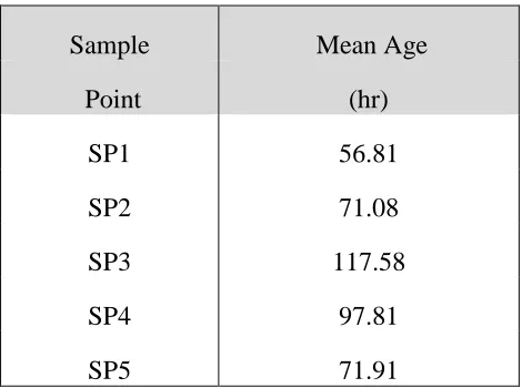
Figure 2 shows the mean water age calculated for each of the sample points. Table 1 summarizes the water
mean age at each sample point; the values being taken directly from the water quality simulation output file
rather than interpolation from the visual output in Figure 2. These single values are average 24-hr values
obtained once a stable age pattern had been obtained. From Table 1 it can be seen that the sample points ordered
- 11 -
Water quality
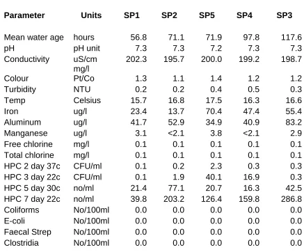
Table 3 presents a summary of the results of the analysis of the water quality samples as site specific, time
averages. This provides a general overview of water quality at each sample point over the 5 day sampling
period. The analytical results are shown in the parameter order presented in Table 2. There were no failures for
regulated parameters. However, there was an order of magnitude difference in site average for 3-day and 7-day
plate counts across the sample sites. The water quality mean parameter values were plotted with standard
deviation error bars for each sample point, ordered by increasing calculated mean age. As the plots are seeking
to explore trends as a function of simulated water age as a general catch all to water quality as opposed to
deterministic relationships, plotting by age category was deemed most appropriate. Consistent stable results
were noted for pH and conductivity, and no counts were observed for coliform, Ecoli, faecal streptococci or
clostridium perfringens, so these parameters are not presented in a graphical form here. Figures 3 to 7 show the
plots for the other parameters. Figure 3 shows the plots for the physical parameters. Color and turbidity
appeared relatively stable (within the +/- SD error bars). Temperature showed an increase with mean water age
for the first 3 points, then a decrease, followed by another increase. Temperature changes should reflect the
ground temperature and the residence time, or age. The expectation would be a consistent upward trend in
summer and downward in winter rather than the fluctuations seen here. Figure 4 shows plots for the metals. Iron
shows some appreciable fluctuation, however, if SP2 is regarded as abnormally low, the pattern approximates to
that of temperature. Aluminum is relatively stable but increases at SP3 which has the highest mean age.
Manganese is very low and stable. Figure 5 shows free and total chlorine plots. Free chlorine appears to
demonstrate the final stage of an exponential decay curve. Total chlorine shows a decrease as mean age
increases through sample points 1, 2 and 5 but then increases again at sample points 4 and 3. This demonstrates
an inverse relationship to iron and temperature if SP2 value for iron is regarded as low. Figure 6 shows 2-day
and 3-day HPC results. The +/- SD error bars at SP 5 are large, otherwise 2-day and 3-day HPCs appear
relatively constant other than the 3-day counts at SP5 and SP4 which slow some increase. Figure 7 shows the
5-day and 7-5-day HPC count data. Within errors, (SP2 (71.08) and SP3 (117.58) have large error bars), it could be
argued that the general trend for 5-day and 7-day plate counts is to increase with increasing mean age.
Perturbations in the data set as a whole, suggest water quality changes between sample points might not be
- 12 -
whether the maximum age contribution to the mean, and the mix of different aged water supplying SP4 and
SP5, might provide a better association.
Analysis of water mixing at sample points
The water volume mixing and maximum age functionalities in Aquis were used to further investigate the water
age components contributing to the mean water age at the sample points. Figure 8 shows the type of results plot
that provided insight into the mixing of different aged water volumes at the sample points. The pipe colors
represent the mean age of the water in the pipes, and the arrows show the direction of flow. The pie charts
situated at each node give a visual representation of the proportion of mixing occurring; the pie slices represent
the different age contributions to the mean water age. Where the mix was between waters of very similar ages
at, SP1 SP2 and SP3, it was assumed to have negligible effect. The other sample points, SP4 and SP5, were
receiving water comprised of a mixture of significantly different aged water volumes. The pop up box in Figure
8 shows the detail of the waters from two directions mixing at SP4, highlighting the fraction of each pipe flow
volume mixed, and the calculated mean age at this point. The age fraction shows that 80.7% of the water at this
location is between 3 and 4 days old and 19.3% is between 6 and 7 days old with a mean of just over 4 days. At
SP5 the age fraction shows that 95.6% of the water is between 2 and 3 days old, 4.4% is between 7 and 8 days
old, and the mean age at the peak flow condition is 72 hours. These results were based on mixing mean age
volumes at the nodes. However, more detailed analysis using Aquis was used to calculate the maximum age
contributions to these mean age volumes i.e. the oldest water volumes were identified.
Maximum Age Analysis
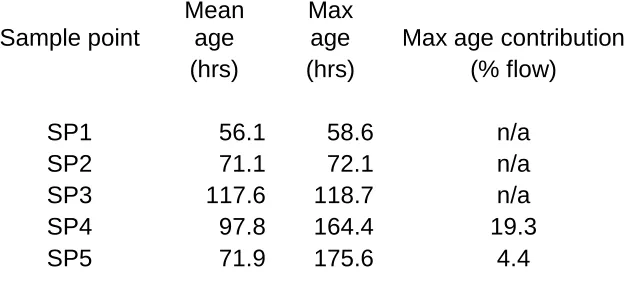
Figure 9 shows the maximum age profiles at the sample points, summarized in Table 4. The maximum age
values in Table 4 were taken directly from the water quality simulation output file rather than interpolation from
the visual output in Figure 8; values are 24 hour averages for day 19 once a stable pattern was firmly
established. From comparison of Table1 and Table 4 it can be seen that the sample point order is different when
consideration is given to maximum age contribution at the sample points when compared to mean age at those
locations. Although it is possible to track all maximum age volumes, where the maximum age differed from
mean age by a relatively small amount (SP1, SP2 and SP3) it was deemed that the maximum age contribution to
water quality would be negligible. The maximum age contribution to flow was only therefore considered for
- 13 -
Water quality analysis - maximum age and volume mixing
The data set was re-ordered to reflect increasing maximum age components at the sample points and the water
quality parameters were re-plotted ordered by sample point maximum age contribution; Figures 10 to 14. Age
categories were again used rather than age values, as no direct mathematical function was being sought i.e.
consideration was being given to age as a general surrogate to water quality. Figure 10 shows the trends for
physical / aesthetic parameters. Color and turbidity appear relatively constant within errors (large error bars for
SP1 and SP5 color for example) however there is a tentative increase with increasing maximum age contribution
albeit by a small amount. Temperature exhibits an unexpected drop at sample points 3 and 4 followed by an
increase to SP5. Figure 11 shows the trends for metals. If SP1 is considered unexpectedly high, iron
concentrations generally increase with increasing maximum age contribution, within analytical tolerances and
errors. This is in contrast to the mean age plot. Aluminum increases from SP1 to SP3 but then decreases. This
apparent decrease may be explained by the dilution effect of younger water merging from SP1 and SP2 prior to
SP5 and SP4 respectively. It may also be indicative of deposition of aluminum due to low flow velocities.
Manganese appears stable at a low concentration. Figure 12 shows the trends for chlorine. When considered
against the maximum age, and within error bars, both free and total chlorine show a decreasing trend with
increasing maximum age contribution, correcting the apparent ambiguity in the mean age plots. This decay law
behavior was anticipated from the literature (Toshiko et al. 2008; Ramos et al. 2010). Figure 13 shows the trends
for 2-day and 3-day HPCs. 2-day and 3-day plate counts both increase with increasing maximum age
contribution, again sorting out the ambiguity seen in the same plots ordered by mean age; however, there are
large +/- SD values for the “change” values at SP4 and SP5. Figure 14 shows the trends for 5-day and 7-day
HPCs. HPC 5-day and 7-day trends are similar when ordered by maximum age contribution, showing an
increase from SP1 to SP3 (assuming HPC 5-day at SP3 is low) then a reduction in values at SP4 and SP5 that
could be due to mixing with younger water at these locations effectively diluting the numbers of heterotrophs.
DISCUSSION
Modeling
It is important to remember that hydraulic and water quality models can only be as good as the data used to
create and drive them. Calculated water age and maximum age contribution is dependent upon the accuracy of
- 14 -
always present and, in such a small area of a network with low flow velocity industrial demand patterns the
propensity for error is appreciable. In particular the exact nature and magnitude of flow routes around low flow
loops, such as studied here, has low certainty for a pressure only calibrated model, yet informative information
has been demonstrated here. In the future work will need to be completed to reduce such modeling uncertainties
before water age (mean and/or maximum) or more deterministic modeling could be used in a regulatory context.
But, this work does demonstrate the potential use of age predictions, using models built to current pressure only
calibration standards, to both understand past water quality failures, as well as to proactively identify possible
problem areas in a network.
Sampling
As regulatory water quality within the network was 99.9% compliant, it was anticipated that small changes in
water quality were being sought to demonstrate the water age / water quality relationship. Sampling did not
account for possible source water quality variation, although this is likely to have been minimal over 1-week
duration, or the time required for a given volume of water to travel between each of the sample points. In the
ideal scenario the water volume sampled at sample point 1 should have been tracked through the network to
ensure the same water volume is sampled at the other sample points; as only by doing this would the true effect
of increasing water age on water quality be measured. However, this was deemed practically prohibitive, and
instead it was decided to try to obtain representative mean values from intensive sampling. Elevated iron
concentrations noticed in some of the first 6 am samples were thought to be due to rust from the stand pipes due
to chlorine disinfection and 18 hours standing. It was therefore decided to take 2 minute and 5 minute flushed
samples from each sample point on days 3, 4 and 5 on the 6am sample round to see if there was a measurable
change in water quality; as 2 minute sample results would have been more reflective of the influence of the
standpipes rather than anything else. Despite taking care setting hydrant flows prior to embarking on the
sampling program some variations in network pressure, and therefore flow rate from the hydrants, was evident
during the sampling period. SP5 hydrant was observed as having the lowest flow. Replicate samples would have
been very useful to enable re-analysis of physical and metal parameters where sample results appeared unusual.
Replicate bacteriological samples would have given higher confidence in HPC results.
- 15 -
Calculating mean water age in a distribution network provides a reasonable overview of the age profile across
the network. However, it is clear that such calculations overlook what could be very important water volumes
that have a much higher age than the average, but which are “lost” in the math used to calculate the mean age
due to the flow weighted mass balance average calculation performed at nodes, Machell et al. (2009).
Considering the water quality analytical results ordered by mean age, and by maximum age contribution to the
mean, the following observations were made.
Physicals
Although color and turbidity appeared relatively constant (within the large error bars for point 1 and point 5 for
example) it could be argued that they increase with increasing maximum age contribution; albeit by a small
amount. The decrease in turbidity at the final point may be explained by the dilution effect of water mixing from
the first point; which would infer that the color figure for the last point is also slightly low for the same reason.
After 3 consecutive increases with increasing mean age, temperature exhibits an unexpected drop followed by a
further increase at the final point. During summer months it would be expected that the longer water is in a pipe
the more heat is transferred from the surroundings resulting in an overall net increase in temperature with
increasing water age. This pattern persists when ordered by maximum age contribution, except it drops after 2
consecutive increases. This unusual pattern could possibly be attributed to local environmental factors, for
example, ground surface material (tarmac / soil / concrete), openness of site, or depth of pipe at the sample
points. However, if points 2, 3 and 4 are considered similar within the error bars, it could be argued that there is
a tendency for temperature to increase with increasing maximum age contribution.
Metals
Analysis of the metals results with respect to maximum age improved the understanding of the processes
occurring with iron showing a clear increase with maximum age contribution as compared to mean age. The
iron results will have been influenced by the excess residence time and corrosion to SP5, and the tidal flow at
SP4, but these effects are still too low to influence color and/or turbidity. Aluminum shows overall dilution
effects caused by the network mixing at SP4 and SP5.
- 16 -
Ordering free and total chlorine by maximum age contribution, Figure 12, rectifies the apparent anomaly shown
in Figure 7, where total chlorine appeared to increase with increasing water age. Figure 15 highlights this
change for total chlorine, with mean age on the primary x-axis and maximum age on the secondary x-axis. This
finding supports the argument that it is necessary to consider the maximum age contribution to understand
chlorine residual response. Comparison of Figures 5 and 12 show how consideration of maximum age can
improve the understanding of changes in chlorine concentrations, total chlorine in particular. This improvement
is notable, as while most chlorine modeling is a stage closer to deterministic modeling than the surrogate of
water age, lumped first, or occasionally second order expressions are used to capture the reactions and
interactions occurring making the assumption of flow weighted mixing at nodes as mean water age modeling.
As with water mean age calculations, this assumption of flow weighted averaging is suspect for chlorine
modeling. For example, it is well known that following secondary chlorination different reaction kinetics occur
(Boccelli et al. 2003, Carrico and Singer, 2009 ). Hence, the decay characteristics of mixed water comprising higher chlorine residual (younger water) mixed with lower chlorine residual (older water) will not
necessarily have the characteristics of the average concentration with the original rate coefficient. This
highlights one of the limitations of currently applied approaches to chlorine modeling in complex networks.
Bacteriological
No coliforms, E-coli, clostridia or faecal streptococci were detected in any of the samples thereby justifying the
need for the suite of heterotrophic plate counts to differentiate small quality changes. Figure 16 highlights the
added insight gained by consider both mean and maximum age for 3-day HPC, similar changes are evident for
2-day HPC but to a lesser extent. 3-day plate counts ordered by maximum age contribution in Figure 16,
produces an increasing trend (within large error bars at points 4 and 5) that is inverse to the total chlorine
pattern, Figure 15. Figure 17 shows the effect of ordering 7-day HPC with mean or maximum age contributions.
Again 5-day counts show similar but not as strong trends. Within the large error bars at points 1 and 3 it could
be argued that the general trend for 5-day and 7-day plate counts is to increase with increasing mean age, again
inverse to chlorine trends. Although HPC levels in this investigation are relatively low, 3-day and 7-day counts
reveal order of magnitude increases over the sampling period suggesting a lowering of water quality with
increasing water age, whether by mean or mixing and maximum age contribution. The difference in trend
between 2-day and 3-day, and 5-day and 7-day counts reflects extra information about slower growing
- 17 -
UK regulations state that there should be “no abnormal change” in HPC counts, i.e. measurements should show
no sudden or unexpected increases, as well as no significant rising trend over time (for repeat sampling of a
site). HPC cannot “fail” in the literal regulatory sense, but investigative sampling should be implemented if
there is sudden change or unexpected increase with time and, presumably, this could/should apply to time spent
in the network as well as over a period of time monitoring a particular site.
In summary, it could be argued from the evidence presented that there is a relationship between water age and
the associated water quality. However, a strong relationship is not demonstrated and perturbations in the results
suggest other influencing factors are at play.
Further work should try to reduce uncertainties in asset material and hydraulic model demand allocation data.
Benefit might also be obtained by undertaking a longer duration sampling program (weeks or months rather than
days) and including all the hydrants in the area (rather than a select few), and source water variations should be
monitored throughout.
CONCLUSIONS
This work produced limited evidence of the association between calculated age of water and water quality
characteristics. Although not deterministic, this is a notable result for a well performing distribution network in
which no water quality events occurred and hence only small changes in water quality parameter were evident;
and these approaching detection limits for many parameters. Mean age proved limited association with general
water quality, and it was necessary to consider mixing effects, and the maximum age component, to obtain some
association as demonstrated by iron, chlorine, and HPCs.
Neither mean nor maximum age approaches fully explained the observed patterns of water quality change in this
localized area of the network. Reasons for this could include model uncertainty, especially in the diurnal
demand patterns, lack of knowledge about the true condition and the bacteriological colonization within the
pipes, and source water variation. However the findings do highlight the limitations of flow/volume weighted
and complete mixing at node assumption made in most modeling software, and the need for research and
development in this area.
- 18 -
The authors wish to acknowledge Yorkshire Water Services’ support for this project and for providing access to
the distribution network. Acknowledgement is also given to the support from EPSRC grant no EP/G029946/1.
REFERENCES
7-Technologies A/S, Bistruphave 3 DK-3460 Birkerød Denmark. Telephone (+45) 45 900 700, Fax (+45) 45
900 701, E-mail [email protected]
American Water Works Association (AWWA - with assistance from Economic Engineering Services). (2002).
“Effects of water age on distribution system water quality”, Total Coliform Rule, Distribution System White
Papers. <http://www.epa.gov/safewater/disinfection/tcr/pdfs/whitepaper_tcr_waterdistribution.pdf>,
(02/04/2007).
Beech, I.B., and Sunner, J. (2004). “Bio-corrosion: towards understanding interactions between biofilms and
metals”. Current Opinion in Biotechnology. 15, 181-186.
Berry, D., Xi, C.W. and Raskin, L. (2006). “Microbial ecology of drinking water distribution systems”. Current
Opinion in Biotechnology. 17, 297-302
Boccelli D. L., Tryby M.E., Uber J.G., Scott Summers, R. (2003). “A reactive species model for chlorine decay
and THM formation under rechlorination conditions”. Water Research. Volume 37, Issue 11, June 2003, Pages
2654-2666
Burllingame, G.A., Korntreger, G., and Lahann, C. (1995). “Configuration of standpipes in distribution affects
operations and water quality”. Journal of the New England Water Works Association. 95 (12), 281-289.
Camper, A.K. (2004). “Involvement of humic substances in regrowth”. International Journal of Food
Microbiology. 92, 355-364.
Carrico, B. and Singer, P.C. (2009). “Impact of Booster Chlorination on Chlorine Decay and THM Production:
Simulated Analysis”. Journal of Environmental Engineering, Volume 135, Issue 10.
- 19 -
Chung, W., Kim, I., Yu, M., and Lee, H. (2003) “Water Quality Variations on Water Distribution Systems in
KOREA According to Seasonal Varying Water Temperatures” World Water and Environmental Resources
Congress 2003, Philadelphia, ASCE, Pennsylvania, USA, June 23–26, 2003.
Emtiazi, F., Schwartz, T., Marten, S. M., Krolla-Sidenstein, P., Obst, U. (2004). “Investigation of natural
biofilms formed during the production of drinking water from surface water embankment filtration”. Water
Research. 38, 1197-1206
Hass, C.N., Meyer, M.A., and Paller, M.S. (1984). “Microbial alterations in water distribution systems and their
relationship to physio-chemical characteristics”. Journal of the American Water Works Association. 75 (9),
475-481.
Keinnen-Toivola, M.M., Revetta, R.P., Santo Domingo, J.W. (2006). “Identification of active bacterial
communities in a model drinking water biofilm system using 16S rRNA-based clone libraries”. FEMS
Microbiology Letters. 257, 182-188
Kirmeyer, G.J. (2000). “Guidance manual for maintaining distribution system water quality”, American Water
Works Association and American Water Works Association Research Foundation. ISBN 1583210741, catalog
number 90798.
LeChevallier, M.W., Babcock, T.M. and Lee, R.G. (1987). “Examination and characterization of distribution
system biofilms”. Appl. Environ. Microbiol. 53, 2714–2724.
LeChevallier, M.W. (1990). “Coliform regrowth in drinking water - a review”. Journal American Water Works
Association. 82, 74-86.
LeChevallier, M.W., Welch, N.J. and Smith, D.B. (1996). “Full-scale studies of factors related to coliform
- 20 -
Machell J., Boxall J.B., Saul A.J., and Bramley, D. (2009). “Improved Representation of Water Age in
Distribution Networks to Inform Water Quality”. Water Resources Planning and Management ASCE. 135 (5),
September, pp 382-391. ISSN 0733-9496. DOI 10.1061/(ASCE)0733-9496(2009)135:5(382)
Mutoti, G., Dietz, J.D., Imran, S., Taylor, J, and Cooper, C.D. (2007). “Development of a novel iron release flux
model for distribution systems”. Journal of the American Water Works Association. 99 (1), 102-111
Niquette, P., Servais, P., Savoir, R., (2001). “Bacterial dynamics in the drinking water distribution system of
Brussels”. Water Research. 35, 675-682
Percival, S.L., and Walker, J.T. (1999). “Potable water and biofilms: a review of the public health implications”.
Biofouling. 14, 99-115
Prasad, T.D. and Walters, G.A. (2006). “Minimizing residence times by rerouting flows to improve water
quality in distribution networks”. Engineering Optimization. 38 (8), 923-939.
Prévost, M., Rompré, A., Baribeau, H., Coallier, J. and Lafrance, P. (1997). “Service lines: their effect on
microbiological quality”. J. Am. Water Works Assoc. 89(7), 78–91.
Ramos, Helena M., Loureiro, D., Lopes, A., Fernandes, C., Covas, D., Reis, L.F., and Cunha, M.C. (2010).
“Evaluation of Chlorine Decay in Drinking Water Systems for Different Flow Conditions: From Theory to
Practice”. Water Resources Management. Volume 24, Number 4, 815-834, DOI: 10.1007/s11269-009-9472-8
Regan, J.M., Harrington, G.W., Baribeau, H., De Leon, R., Noguera, D.R. (2003). “Diversity of nitrifying
bacteria in full-scale chloraminated distribution systems”. Water Research. 37, 197-205
Reilly, K.J. and Kippin, J.S. (1983) “Relationship of bacterial counts with turbidity and free chlorine in two
- 21 -
Rossman, L.A, Clark, R.M., and Grayman, W.M. (1994). “Modeling chlorine residuals in drinking water
distribution systems”. Journal of Environmental Engineering. ASCE, 120 (4), 803-820
Speh, K., Thofern, E. and Botzenhart, K. (1976). “Untersuchungen zur Verkeimung von Trinkwasser. IV.
Mitteilung: Das Verhalten bakterieller Flächenbesiedlungen in einem Trinkwasserspeicher bei Dauerchlorung”.
GWF-Wasser/Abwasser. 117, 259 – 263.
Standing Committee of Analysts. (1998). “The history and use of HPC in drinking-water quality management”.
http://www.who.int/water_sanitation_health/dwq/HPC3.pdf Last accessed 15:05 25-05-2001
Standing committee of analysts. (2002). “The Microbiology of Drinking Water 2002 – Part 3 – Practices and
Procedures for Laboratories. Methods for the Examination of Waters and Associated Materials”. Environment
Agency. http://www.environment-agency.gov.uk/static/documents/Research/mdwpart3.pdf
Last accessed 15:22 09/08/2011
Srinivas Panguluri, Radha Krishnan, Lucille Garner, Craig Patterson, Yeongho Lee, David Hartman, Walter
Grayman, Robert Clark, and Haishan Piao. (2005). “Impacts of Global Climate Change.” Proceedings of World
Water and Environmental Resources Congress. 2005 ISBN: 0-7844-0792-4 Publisher: ASCE
Szewzyk, U., Szewzyk, R., Manz, W., Schleifer, K.H. (2000). “Microbiological safety of drinking water”.
Annual Review of Microbiology. 54, 81-127.
Toroz, I. and Uyak, V. (2005). “Seasonal variations of trihalomethanes (THMs) in water distribution networks
of Istanbul City”. Desalination. 176 (1-3), 127-141
Toshiko N., Tomohiro F., Katsuhiko T. (2008). “Residual Chlorine Decay Simulation in Water Distribution
System”. The 7th International Symposium on Water Supply Technology, Yokohama, Japan
UKWIR (2006). “Bacteriological indicators of water quality”. Report Ref. No. 05/DW/02/41. ISBN: 1 84057
- 22 -
Water Science and Technology Board. (2005). “Public water supply distribution systems: assessing and
reducing risks, First Report”. Committee on Public Water Supply Distribution Systems: Assessing and Reducing
Risks. National Research Council, National Academy Press, October 2005, ISBN-10: 0-309-09628-6, ISBN-13:
978-0-309-09628-7, ISBN/SKU 0309096286.
Wu, C. G., Wu, Y., Gao, J. L., and Zhao, Z. L. (2005) “Research on water detention times in water supply
- 23 -
Figure captions
Figure 1. Calculated water mean age profiles at the sample points
Figure 2. Network layout, sample point locations, flow routes and mean age
Figure 3. Color, turbidity and temperature ordered by sample point mean age
Figure 4. Iron, aluminum and manganese ordered by sample point mean age
Figure 5. Free and total chlorine ordered by sample point mean age
Figure 6. 2-day and 3-day plate counts ordered by sample point mean age
Figure 7. 5-day and 7-day plate counts ordered by sample point mean age
Figure 8. Mixing of different aged water volumes
Figure 9. Maximum age profiles at the sample points
Figure 10. Color turbidity and temperature ordered by sample point maximum age contribution
Figure 11. Iron, aluminum and manganese ordered by sample point maximum age contribution
Figure 12. Free and total chlorine ordered by sample point maximum age contribution
Figure 13. 2-day and 3-day HPCs ordered by sample point maximum age contribution
Figure 14. 5-day and 7-day plate counts ordered by sample point maximum age contribution
Figure 15. Total chlorine residual ordered by mean age and maximum age contribution
Figure 16. 3- HPC ordered by mean age and maximum age contribution
- 24 -
Table captions
Table 1. Water mean age at water quality sample points
Table 2. Analytical parameters
Table 3. Summary of water quality results (ordered by mean age at sample point)
Table 4. Maximum age of the water volumes at the sample points, and the maximum age volume contribution to
- 25 -
Sample
Mean Age
Point
(hr)
SP1
56.81
SP2
71.08
SP3
117.58
SP4
97.81
[image:26.595.71.306.93.268.2]SP5
71.91
- 26 -
Physical
Chemical
Biological
pH
Iron
HPC 2-day @ 37
oC
Conductivity
Aluminium
HPC 3-day @ 22
oC
Colour
Manganese
HPC 5-day @ 30
oC
Turbidity
Free chlorine
HPC 7-day @ 22
oC
Temperature
Total chlorine
Total coliforms
Ecoli
Clostridium perfringens
[image:27.595.76.450.105.323.2]Faecal streptococci
- 27 -
Parameter
Units
SP1
SP2
SP5
SP4
SP3
Mean water age hours
56.8
71.1
71.9
97.8
117.6
pH
pH unit
7.3
7.3
7.2
7.3
7.3
Conductivity
uS/cm
202.3
195.7
200.0
199.2
198.7
Colour
mg/l
Pt/Co
1.3
1.1
1.4
1.2
1.2
Turbidity
NTU
0.2
0.2
0.4
0.5
0.3
Temp
Celsius
15.7
16.8
17.5
16.3
16.6
Iron
ug/l
23.4
13.7
70.4
47.4
55.4
Aluminum
ug/l
41.7
52.9
34.9
40.9
83.2
Manganese
ug/l
3.1
<2.1
3.8
<2.1
2.9
Free chlorine
mg/l
0.1
0.1
0.1
0.1
0.1
Total chlorine
mg/l
0.1
0.1
0.1
0.1
0.1
HPC 2 day 37c
CFU/ml
0.1
0.2
2.3
0.3
0.3
HPC 3 day 22c
CFU/ml
0.1
1.9
40.1
16.9
0.3
HPC 5 day 30c
no/ml
21.4
77.1
20.7
16.3
42.5
HPC 7 day 22c
no/ml
39.8
203.2
126.4
159.8
286.8
Coliforms
No/100ml
0.0
0.0
0.0
0.0
0.0
E-coli
No/100ml
0.0
0.0
0.0
0.0
0.0
Faecal Strep
No/100ml
0.0
0.0
0.0
0.0
0.0
[image:28.595.71.508.92.454.2]Clostridia
No/100ml
0.0
0.0
0.0
0.0
0.0
- 28 -