Article:
Masood, S., Fang, R., Li, P. et al. (8 more authors) (2019) Automatic choroid layer
segmentation from optical coherence tomography images using deep learning. Scientific
Reports, 9 (1). 3058.
https://doi.org/10.1038/s41598-019-39795-x
[email protected]
https://eprints.whiterose.ac.uk/
Reuse
This article is distributed under the terms of the Creative Commons Attribution (CC BY) licence. This licence
allows you to distribute, remix, tweak, and build upon the work, even commercially, as long as you credit the
authors for the original work. More information and the full terms of the licence here:
https://creativecommons.org/licenses/
Takedown
If you consider content in White Rose Research Online to be in breach of UK law, please notify us by
Automatic Choroid Layer
Segmentation from Optical
Coherence Tomography Images
Using Deep Learning
Saleha Masood , Ruogu Fang , Ping Li
, Huating Li , Bin Sheng
, Akash Mathavan ,
Xiangning Wang , Po Yang , Qiang Wu , Jing Qin & Weiping Jia
The choroid layer is a vascular layer in human retina and its main function is to provide oxygen and support to the retina. Various studies have shown that the thickness of the choroid layer is correlated with the diagnosis of several ophthalmic diseases. For example, diabetic macular edema (DME) is a leading cause of vision loss in patients with diabetes. Despite contemporary advances, automatic segmentation of the choroid layer remains a challenging task due to low contrast, inhomogeneous intensity, inconsistent texture and ambiguous boundaries between the choroid and sclera in Optical Coherence Tomography (OCT) images. The majority of currently implemented methods manually or semi-automatically segment out the region of interest. While many fully automatic methods exist
in the context of choroid layer segmentation more e ective and accurate automatic methods are
required in order to employ these methods in the clinical sector. This paper proposed and implemented an automatic method for choroid layer segmentation in OCT images using deep learning and a series of morphological operations. The aim of this research was to segment out Bruch’s Membrane (BM) and choroid layer to calculate the thickness map. BM was segmented using a series of morphological operations, whereas the choroid layer was segmented using a deep learning approach as more image statistics were required to segment accurately. Several evaluation metrics were used to test and compare the proposed method against other existing methodologies. Experimental results showed that the proposed method greatly reduced the error rate when compared with the other state-of-the-art methods.
he choroid layer is vital for the oxygenation and metabolic activity of the Retinal Pigment Epithelium (RPE) and outer retina. It is a vascular interface between the retina and sclera and requires some of the highest amounts of blood low for any tissue in the human body. he choroid layer also acts as a source of blood supply for the optic nerve1. he structure of the layer is mainly divided into two parts based on anatomical structure: the vascular plexus, consisting of various capillaries contiguous to BM, and the choroidal stroma. Changes in the shape and anatomical structure of the choroid have been acknowledged in primary macular degeneration and in other advanced diseases. Quantitative and qualitative analysis of BM and the choroid layer can help in understanding the relationship between these various retinal diseases.
Optical coherence tomography (OCT) is an increasingly signiicant modality for the identiication, moni-toring, and measurement of many retinal and macular diseases as it aids in resolving cross-sectional details of the human retina. he growing need for OCT in retinal disease analysis necessitates investigation into a fully
Department of Computer Science and Engineering Shanghai Jiao Tong University Shanghai China J. Crayton Pruitt Family Department of Biomedical Engineering University of Florida Gainesville FL USA Faculty of Information Technology Macau University of Science and Technology Macau China Shanghai Jiao Tong University A liated Sixth People s Hospital Shanghai China Department of Computer Science, Liverpool John Moores University Liverpool L AF UK Centre for Smart Health School of Nursing The Hong Kong Polytechnic University Hong Kong China Saleha Masood Ruogu Fang Ping Li and Huating Li contributed equally. Correspondence and requests for materials should be addressed to B.S. (email: shengbin@sjtu. edu.cn) or Q.W. (email: wyansh com)
Received: 27 March 2018
Accepted: 21 January 2019
Published: xx xx xxxx
automated approach2. Useful information can be extracted with the blend of OCT, image processing, and seg-mentation techniques. his can provide detailed information regarding diferent retinal layers and the associated diseases. DME, a chief source of vision damage in patients sufering from diabetes, can be diagnosed with the help of choroid thickness maps as changes in thickness, such as those resulting from choroidal macular degen-eration and other advanced diseases, can provide a relative measure of health of the choroid layer. Aging may also cause choroidal thinning that leads to a condition referred to as choroidal atrophy3,4. Increased choroidal thickness can result in diseases like serous retinopathy, polypoidal choroidal vasculopathy, autoimmune diseases, etc. Early diagnosis of these diseases can prove to be very beneicial in the treatment of these abnormalities. hus, quantiication of pathological changes can be efectively achieved by the analysis of retinal thickness and, for such diagnoses, choroidal thickness measurement is essential5,6.
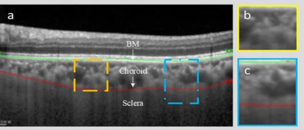
In OCT imaging, some approaches ind the correlation among the measurable and morphological topogra-phies of retinal thickness maps7. Such normal standards for the thickness maps can help physicians in comparing diferent patients’ choroidal thickness maps with normal sets. Consequently, the automatic segmentation of the choroidal boundary has garnered the attention of many researchers worldwide. A review of existing approaches in this domain shows that not much work has been carried out for automatic segmentation of the choroid layer, as most methods only manually or semi-automatically segment out the region of interest. Manually outlining the choroid boundary is a tedious, time consuming and sometimes impossible task because of possible indistinct structures and boundaries. Moreover, the measurement lacks objectivity, requires the trainer to be trained per-fectly, and is vulnerable to inter-observer imprecision8,9. Also, while some fully automatic segmentation methods do exist, there is still room for improvement. Major challenges in the accurate segmentation of the choroid layer are visualized in Fig. 1 and are detailed as follows:
• Low contrast of OCT images makes the region between the sclera and choroid inseparable, resulting in a likewise inseparable histogram between the two layers
• Methods based on thresholding and intensity are not efective because of the aforementioned low contrast in OCT images
• Due to the presence of the vascular structure, the choroid layer has inconsistent texture and inhomogeneous intensity that makes extraction of the region of interest diicult
• he anatomical structure of BM and the choroid layer interface is quite weak and is oten invisible
In consideration of current challenges within the choroid segmentation domain, the major contributions of this work include:
• A two-stage segmentation approach with emphasis on segmentation accuracy and consistency of the method • OCT image segmentation based on the combination of morphological and deep learning methodologies • Testing on the data of real patients, with experimental outcomes showing that the technique achieved high
precision and reduced error rates to a signiicant extent
he remainder of the paper is structured as follows: Section 2 outlines literature review. Proposed method-ology details are described in Section 3. Experimental results with a quantiiable examination are presented in Section 4. Finally, the conclusion and future directions are discussed in Section 5.
Related Work
Existing literature in the context of choroid layer segmentation includes manual, semi-automatic and few auto-matic segmentation methods in OCT images. As the prime objective of this research focuses on the use of deep learning methodologies, the literature review is divided into two subgroups: deep learning methods and non-deep learning methods.
[image:3.595.164.477.48.182.2]Machine learning is a method of data analysis that employs statistical and analytical tools on training data. hese tools are later used to learn from past examples and employ the learned information from the preceding
training to categorize new data, envisage new inclinations and ind new patterns. Image classiication or segmen-tation is one of the fundamental methods in the domain of machine learning. Analysis of literature shows the use of several, non-deep learning, traditional methods such as graph-based, k-nearest neighbor, Bayesian network, support vector machine and decision tree approaches, all of which involve the use of hand-crated features for the speciic classiication purpose. he hand-crated features include shape, pixel density and texture of the image features.
In the context of these non-deep learning methods, a previous automatic choroid layer segmentation method was used to extract choroidal vessels for quantiication of choroidal vasculature thickness10. his approach focused on the thickness of vessels rather than the choroid layer. Another automatic segmentation technique11 applied a statistical model on choroid layers in OCT images. However, the processing time of the method is quite high and extensive training is required. Use of phase information for automatic segmentation of the interface between the choroid and sclera was proposed and implemented12,13. While successful, these methods are not clinically practical as the used imaging modalities are not commercially obtainable. he use of dynamic program-ming (DP) in one study was used to ind the shortest path of a graph for choroid layer segmentation, giving a seg-mentation accuracy of about 90 percent8. Additionally, a two-stage active contour model for choroidal boundary extraction with a segmentation accuracy of 92.7 percent was proposed14. Graph based approaches have also been used in this context but, due to the heterogeneous nature of OCT images, these methods are not generally helpful in choroid layer segmentation15–17. Still, one study utilized a graph search algorithm from 3D OCT volumes to perform choroid layer segmentation18. his method was a semi-automatic approach. he interface between the choroid and sclera using Dijkstra’s algorithm was investigated9.
OCT B-scan choroidal segmentation based on a dual probability gradient has also been attempted19. Another study presented an automatic segmentation method based on a multi-resolution textural graph cut method16. he combination of Markov Random Field (MRF) and level set approach was also used to segment the choroid layer20. Distance regularization and edge constraint terms were rooted into the level set technique to evade une-ven and trivial areas and preserve information around the boundary between the choroid and sclera. MRF based methods21–23 have been proposed and implemented to detect the intra-retinal layers from 2D or 3D OCT images. Another method focused on obtaining the spatial distribution of choroidal sub-layers with 3D 1060-nm OCT mapping using Haller’s and Sattler’s layer24. A hybrid approach has made the use of level set, multi-region con-tinuous max-low method to segment out diferent retinal layers. he approach also used nonlinear anisotropic difusion in order to eliminate the spackle noise present in the OCT images25. Seven layers of the retina were also segmented in this context; the proposed approach involved a combination of graph cut and dynamic program-ming26. Two sequential difusion map based segmentations of intra-retinal layers from 3D SD-OCT scans have been developed27. A similar approach for the segmentation of multiple retinal layers utilized spectral rounding for segmentation28.
Review of Recent Deep Learning Techniques in Computer Vision.
he conducted literature review showed that most of the existing choroid layer segmentation approaches made use of non-deep learning meth-odologies. An overview of existing deep learning methods revealed that, in this context, these methods are not used speciically for the choroid layer segmentation. hey are generally applied in medical image segmentation, such as on the brain, retina, liver, knee, urinary bladder, chest, heart, etc. Deep learning is a branch of Artiicial Intelligence (AI) with the ability to make use of optimization, probabilistic and statistical tools; these methods maintain an extensive contribution to the analysis of medical images.With regard to biomedical image segmentation, one major study contributed an approach for the segmenta-tion of biomedical image segmentasegmenta-tion using Convolusegmenta-tional Neural networks (CNNs)29. he model employed a network and training strategy that relied on the robust use of data augmentation. Low grade glioma assessment through a modiied CNN architecture with 6 convolutional layers and a fully connected layer was used to clas-sify these brain tumors30. A similar approach was used in the diagnosis of white matter hyperintensities from brain MRI images through a series of CNN architectures that considered multi-scale patches to yield the obvious position of required features while training31. Another group proposed an automatic computer-aided diagno-sis method for the classiication of solid and non-solid nodules in pulmonary computerized tomography (CT) images through a CNN32. Brain image segmentation to produce high nonlinear mappings between inputs and outputs using deep learning was analyzed; the segmentation problem was solved using CNNs33,34. he approach made use of local features in conjunction with more global contextual features to perform the segmentation. Other studies have investigated the use of automatic segmentation and assessment of rectal cancers from the multi-parametric MR images through the use of CNN architectures35. he combination of CNN and total kidney volume calculation from Computed Tomography for the segmentation has been proposed in36. he method was tested on the images of real patients demonstrating trivial to adequate function to severe renal inadequacy. he detection of bladder cancer has also incorporated use of CNN architectures in a combination with level set meth-ods to acquire the region of interest37.
segmentation of retinal layers has not observed in existing methods of deep learning. As OCT imaging tech-nology allows capturing of the cross-section of the retina, it may be very helpful to analyze OCT images for the diagnosis of several retinal diseases. Because choroid layer segmentation and associated thickness measurements help diagnose retinal based diseases, several approaches have been proposed and implemented to diagnose them. For instance, retinitis pigmentosa42, central serous chorioretinopathy43, age-related macular degeneration44, and diabetic retinopathy45,46 have been found to have associated changes in the thickness of the choroid.
One study showed the development of an automatic method for the segmentation of retinal layers based on deep learning methodologies, highlighting one of only few current implementations of an automatic technique. he method made use of CNN to perform the retinal layer segmentation in OCT images47. he procedure was limited in accuracy of edge detection as it depended on at most one-pixel accuracy; however, the Bidirectional Long Short-term Memory (BLSTM) entails sub-pixel accuracy. his can lead to confusion in the accurate seg-mentation of the corresponding boundaries. A similar method48 performed OCT image semantic segmentation through fully convolutional neural networks, but the results were tested on a data-set of normal individuals with fewer images of mild spectrum diabetic retinopathy. A combination of CNNs and graph search methods has also been employed in the segmentation of 9 retinal boundaries49. he method was computationally expensive and the black-boxed architecture of the CNN made customization and performance examination of every step less controllable. Segmentation of retinal layers with emphasis on luid masses has also been performed using deep learning methods50. While results were promising, evaluation was conducted on a limited number of B-scans. he tested and training data sets contained a total of 110 B-scans.
According to analysis of the related works, it can be observed that higher segmentation accuracy was achieved through deep learning methodologies. he key restraint of non-deep leaning approaches is that these methods mainly rely on the feature extraction phase for the accurate segmentation of the region of interest. It is tough to extract appropriate image features for a deinite medical image recognition problem. As a result, the classiier cannot provide efective segmentation accuracy because the segmented features are not efective enough. In order to tackle problems faced by non-deep learning approaches, signiicant segmentation accuracy is achieved by the use of deep learning methods through adaptive learning of image features. Considering this, it is likely that the application of deep learning methods on the categorization of OCT images for automated disease diagnosis would be more successful than counterpart non-deep learning procedures. hus, the focus of this research is to overcome existing challenges in choroid layer segmentation and provide a fully realized automatic segmentation approach. he proposed method makes use of deep learning to achieve the desired task, with a combination of morphological operations and CNNs. In order to calculate the thickness map of choroid layer, segmentation was considered for two layers. he desired layers included BM and the choroid layer. BM was segmented out using a series of morphological operations followed by the use of CNNs for choroid segmentation. hen, a thickness map was generated based on the extracted layers.
Material and Methods
Pipeline Overview.
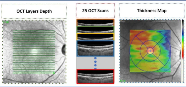
he proposed methodology is a two-stage segmentation process. Quantiication of cho-roidal thickness relies on the extraction of two layers from OCT images. he segmentation of BM was carried out followed by the extraction of choroid layer from the OCT images. Figure 2 represents a standard OCT image with the required layers segmented in diferent colors. he regions of interest are labeled by the experts manually; BM is labeled in green whereas the choroid layer is labeled in red.he proposed method takes a set of OCT images focused on the retina around the macula as input and depicts the position of two required boundaries. As the data of every individual contained 25 B-scans of the macula, the OCT images were comprised of a series of B-scans that the proposed method segmented individually. he result of segmentation of all B-scans was examined, combined and, lastly, incorporated to shape graphical depictions as 2D maps. Initially, we regulated tomography volume data by representing it as a sorted series of adjacent B-scans. Later the images were labeled by image statistics from adjacent B-scans and the region of interest was segmented in every B-scan individually. hen, the 2D retinal and choroidal thickness maps were generated. Figure 3 depicts the procedure carried out to generate the thickness map.
[image:5.595.157.480.50.142.2]he proposed methodology is comprised of 3 main modules including BM segmentation, choroid layer seg-mentation, and thickness map generation. Figure 4 depicts the overall approach of the proposed method. For the segmentation of the regions of interest, OCT images were taken as inputs to the system. he BM was segmented
using a series of morphological operations whereas the segmentation of choroid layer, which required more image statistics, was extracted using a CNN. Later, thickness maps were generated using the extracted layers.
[image:6.595.159.512.48.213.2]Bruch’s Membrane Segmentation.
A series of steps were performed to carry out BM segmentation. If we analyze the OCT image, we can observe that BM segmentation is relatively easier than choroid layer segmen-tation. he reason is that the choroid layer has inhomogenous intensity and inconsistent texture, so it requires more image statistics to accurately segment. We irst segmented the BM followed by segmentation of choroid layer. In this case, we can consider the segmented BM as a constraint while carrying out choroid layer segmen-tation. he segmentation of BM was performed using a sequence of morphological operations. MorphologicalFigure 3. hickness Maps: 25 b-scans of every individual were taken into account to generate a thickness map of an individual.
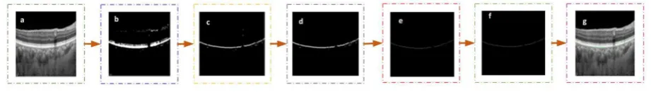
[image:6.595.158.552.266.591.2]operations mainly represent a collection of non-linear operations associated with the morphology or shape of the features in the OCT image. Morphological image processing follows the goal of eliminating all the defects and maintaining structure of the image. hese operations are conident on the associated ordering of pixel values, rather than their numerical values, so they are utilized more on binary images. BM boundary represents a clear white boundary in the OCT image as compared to the other layers/structures in the image. Additionally, as it is evident from the OCT images, the intensities of the BM boundary are homogeneously distributed. he histogram peaks corresponding to BM are distinct from each other as well as from the background. he distinctive feature of the proposed method is that it ensures the homogeneous intensity distribution for the BM boundary. his helped to improve the visibility of delicate mass lesions and helped to reduce unwanted background information. A summary of the performed steps are shown in Fig. 5. he steps involved in this process are detailed as follows:
Thresholding.
he irst step was to convert the image into binary and extract the region of interest. he reason behind this step was to extract the pixels containing the region belonging to the BM boundary within the image. In order to obtain an optimal threshold value, OCT images were tested using a range of threshold values. Ater the analysis, the optimal threshold value was set to 190. his step helped determine the foreground and background pixels of the image. he output of the step was binarized data containing a range of intensity values. he threshold was deined as:
∈ ≤ <
∈ ≤ < −
p S P t
p S t P L
if 0
if 1 (1)
ij i j b
ij b i j
( ) 1 ( , )
( ) 2 ( , )
where pi,j, i= 1, 2, …, r, j= 1, 2, …, c represents the pixel intensity of the image (with size r × c and n = L gray
lev-els from zero to L-1), tb is the set threshold, S1 and S2 are sets in which pixels with intensities between thresholds k and k-1 are located. Image was divided into two sets S1 and S2 (background and foreground pixels respectively) using a threshold at the level tb. Here S1= [0, …, tb−1] and S2= [tb, …, L− 1].
Reconstruction.
Ater acquiring the binary image, a reconstruction approach based on the morphologi-cal opening was applied to remove the noise and preserve the shape of BM layer that was not removed by the morphological erosion operator in the OCT image. he block analysis method can be assumed to be similar to this approach based on the fact the image is manipulated as a whole rather than dividing it into blocks. Firstly, a structuring element B of size 3 × 3 was formulated by considering minimum Imin(x) and maximum intensitymax Imax(x). Later, the background benchmarks Ri were deined based on the obtained values. he background
criterion was formulated as:
= +
R x( ) I ( )x I ( )x
2 (2)
min max
where Imin(x) and Imax(x) represents morphological erosion and dilation respectively. herefore,
δ
=
+
µ µ
R x( ) ( )( )f x ( )( )f x
2 (3)
where ϵ represents the erosion operator followed by δ operation and µ represents the structuring element. he employed reconstruction approach yielded better results when compared to the traditional block cutting method as the used method provided better local analysis of the OCT image. Eight neighboring pixels at every point within the OCT images were considered by the structuring element µ.
[image:7.595.96.557.47.112.2]Thinning.
Ater image reconstruction, the number of rows spanned by the objects were taken into account. In order to select the object-spanned rows, a range was deined, given that the rows contained most of the points. Any point outside the selected range was discarded. hen, foreground pixels not part of the BM boundary were eliminated. he morphological thinning operation was applied on the extracted rows containing the BM area in the OCT image. he purpose of this step was to iteratively remove pixels exclusive to the shape and to shrink it without shortening or breaking BM boundary apart. To achieve the desired goal, we observed whether an edge pixel P1 should be removed by considering its 8 neighbors in the 3 × 3 neighborhood. To delete or mark the pix-els, the approach of connectivity numbers was employed. he approach helped us to ind the number of objectsbeing connected to a speciic pixel in the OCT image. he connectivity number was calculated using the following equation:
∑
= −
∈
+ +
⁎ ⁎
C N (N N N )
(4) n
k s
k k k 1 k 2
where No represents the central pixel and the color of eight neighbors is represented by Nk. he pixel to the right
of the central pixel is represented by N1. All remaining neighboring pixels were numbered in counter-clockwise order around the central pixel.
Curve Fitting.
he next step was to mark the boundary of segmented BM. his step was performed using spline curve itting. Curve itting was applied to ind a function f(x) based on the data (xi, yi) where i= 1, 2, …, n.he residual was minimized by the function (x). he residual is the distance between the data samples and f(x). A better curve itting can be obtained through a smaller residual. Spline itting being applied for the curve itting was calculated as:
= − + − + − +
f x( ) a xi( xi))3 b xi( xi)2 c xi( xi) di (5)
where ai, bi, ci an di represents set of polynomial coeicients and xi= 1, 2, …, n represents the data points to be
mapped in the curve. he output of this step is the inal segmented BM boundary. Figure 5 illustrates the output of each step being performed for the BM boundary segmentation; it has 7 subparts, each representing a result of the diferent morphological operations being applied on the input OCT image.
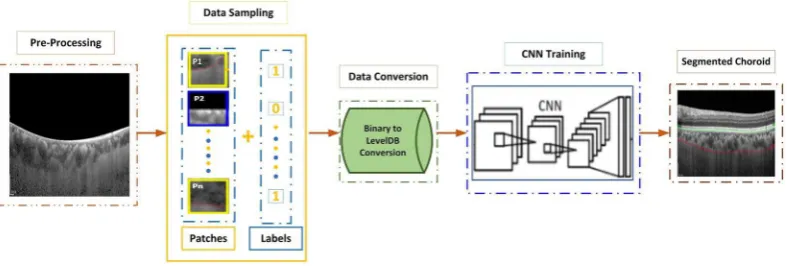
Choroid Layer Segmentation Using Deep Learning.
As discussed above, BM segmentation is easier when compared to the segmentation of the choroid layer. Based on the the aforementioned challenges and provi-sions, a deep learning approach was taken to carry out the desired segmentation.Figure 6 illustrates the steps that constituted the segmentation process. hese steps include pre-processing, data sampling, data conversion, CNN training and inal choroid layer segmentation.
Pre-Processing.
In the pre-processing phase, the segmented BM was kept as a point. All points in the area above the reference point were set to black. his was to reduce the area to be processed for the segmentation of the choroid layer. he output of BM segmentation (the segmented layer) was fed as an input to this stage. Analysis of the OCT image showed that the interface between the sclera and choroid layer is inseparable in the majority of cases and, as a result, accurate segmentation of the choroid layer is a challenging task. Based on this analysis, the purpose of the pre-processing stage was to obtain the deinite region of the OCT image containing the choroid layer. Consequently, the pre-processing step simply eliminated all of the area above the segmented BM.Data Sampling.
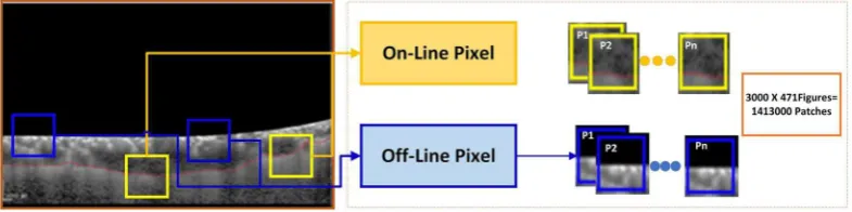
he data provided by the doctors contained manually segmented BM and choroid layers. he segmentation of the required boundaries on OCT images was performed by the experts manually. he data sampling step made use of the provided data to sample the patches to be used for training of the CNN. he man-ually segmented images were sampled patch-wise from top to bottom and let to right. he purpose of sampling was to classify pixels as on-line or of-line patch. he patch size used in our research was 32 × 32. his patch size was used because:• Very small patch sizes make it diicult to extract useful information from the region of interest • Very large patch sizes may contain surplus information and increase the complexity of processing
As patched images were manually segmented by the ophthalmologist, the choroid layer was marked by a red curve. he classiication of the patches was performed in order to pick the patches containing the choroid layer. he illustration of the patch labeling process is described in Fig. 7.
[image:8.595.158.552.47.180.2]he stride between each patch was taken as 5 pixels. A threshold was then set to discard patches containing too many black pixels. If more than 1/3 of the patch contained black pixels, it was discarded. he data set contained
images of 21 patients. Data of 11 individuals was used to train the model whereas data of 10 individuals was used to test the model. In order to balance labels 0 and 1, the patches of label 0 were randomly chosen to have the same number as label 1. here were almost 3000 patches for one igure, so the total number of patches being sampled from the data was about 1,575,000.
Data Conversion.
Next, we converted the data to binary format. he binary format for CIFAR-10 is shown in Equation 6. Here, the irst image label (i.e. 0 or 1) was represented by the irst byte. Image pixel values were denoted by the next 3072 bytes. Red channel values were indicated through the irst 1024 bytes, the following 1024 bytes represented green channel values and the last 1024 bytes corresponded to blue channel values. Row major order was used to store these values, where an initial 32 bytes represented the red channel in the initial row of the image.<1xlabel><3072xpixel> … … … <1xlabel><3072xpixel> (6)
he next step was to convert the binary ile to leveldb format because cafe only supports leveldb or lmdb51. We used the program provided by Cafe to do this transformation. Ater the transformations, the CNN model was trained using the extracted information. Ater training the model it was used for the segmentation of the choroid layer.
CNN Training.
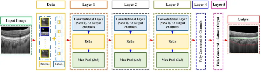
he CNN layering structure used in this work was the Cifar-10 model52. We used a pre-trained CNN Cifar-10 architecture to generate features and trained the network using sampled data. he CNN architec-ture was composed of a layering strucarchitec-ture. he layers of the CNN included layers of convolution, pooling, and linear unit nonlinearities. here was also a linear classiier for contrast normalization on top of all these layers. he modiication was carried out in the last layer of the CIFAR-10 model. he architecture of the CNN used in our approach is shown in Fig. 8.Figure 8 shows the overall structure of the CNN model being used in this work. Because contrast of OCT images was low and the texture between the choroid layer and sclera was inhomogeneous, we preferred to carry out the segmentation through slices being sampled from the OCT images. hus, our model processed each 2D OCT image sequentially in slices. he proposed approach predicted the class of every patch based on the asso-ciated label of the patch. he CNN processed the M×N patch centered on that pixel. herefore the input to the CNN model was an M × N 2D patch. he CNN architecture’s main structuring element was the convolutional layer. In this case, numerous layers can be piled on top of each other to make a pyramid of image features. Each layer in the pyramid harvests features from the prior layer. A stack of input planes was fed to the convolutional layer of our model as its input. he convolutional layer processed the procedures that were being fed and pro-duced feature maps as output. he feature maps were propro-duced by applying spatially local non-linear feature extractors to all spatial neighbors of the input planes. As a result, we obtained an organized topological map of the responses. For the irst convolutional layer, diferent OCT 2D M × N patches were represented through the individual input planes. In successive layers, the input planes were characteristically comprised of the feature maps of the preceding layer. he implemented model contained 5 layers starting with three convolutional layers followed by two fully connected layers. he inal layer of the network was a sotmax layer used for the inal clas-siication. he convolutional layers were followed by max pooling and Rectiied Linear Units (ReLU). Kernels in the convolutional layer were of size 5 × 5 with a step size of 1. he kernels of max pooling layer were of size 3 × 3 with a step size of 2. he convolutional layer mainly performed the feature extraction phase - it helped translate the input to its equivalent characteristics.
[image:9.595.158.551.49.147.2]he pyramid of complex features in the CNN model was considered by giving a convolutional layer’s output feature maps as input channels to the successive layer of convolution. In precise denotation, if focusing on a fea-ture map, it represents a layer of neurons. Each neuron in the layer corresponds to a coordinate within the feafea-ture map. he size of the neuron’s separate ield correlates to the size of the kernel. he connection among the neurons of the same layer and the previous layer is represented by the value (weight) of the kernel. In the learned kernel’s weights, each kernel is adjusted to a diverse orientation, spatial frequency and scale suitable for the training data. Finally, in order to obtain segmentation labels, we connected the convolutional hidden layer to a fully connected layer followed by a fully connected and sotmax layer. As the layers were fully connected, there were 64 output
channels because input channels were 32. Each kernel in the fully connected layer acted as the ultimate detector of the choroid from one of the segmentation labels. he purpose of this layer was to map activation volume from the blend of preceding diferent layers into a class probability distribution. he CNN was trained based on the extracted patches from the OCT images. Test image patches were used to get the overall test accuracy of the pro-posed model and develop an overall understanding of the image classiication as a segmentation procedure for the choroidal boundary.
As discussed in the data sampling and data conversion sections of the methodology, the input OCT image was analyzed with a patch window being traversed on the OCT image. he window size was set to 32 × 32 and the patches were analyzed and given labels according to the contents contained within that window patch. he whole image was traversed and the image was cut into 32 × 32 image slices. As a result, we obtained many patches from a single OCT image. he OCT image was classiied into two classes: part of the choroid layer or not part of the choroid layer. herefore, all patches were classiied into the two classes. he total sampled patches amounted to about 1,575,000 patches, extracted from 525 OCT images of 21 individuals. Data of 11 individuals was used to train the network, meaning 825,000 patches (275 images) were used to train the network. Data of 10 individuals was used to test the network, meaning 750,000 patches (250 images) were used.
Ater sampling patches from all the images, the sampled patches were used to train the model. Figure 9 shows the testing and training phase of the network. he distribution of the segmentation labels was obtained by ana-lyzing the output of the convolutional network. he objective of the training condition was to lessen the negative log-probability from every OCT image by exploiting the likelihood of all labels in the training set being used. his was formulated as:
−Log Y = −
X sum Log
Y
X (7)
max ij max
[image:10.595.102.554.48.173.2]ij
Figure 8. CNN Architecture: he CNN architecture being used in this research entails of a sequence of layers including convolution, rectiied linear units followed by max pooling layer, fully connected and a sotmax layer.
[image:10.595.151.552.220.438.2]parameters of the model with respect to the parameters θ:
∏
θ θ θ θ θ = = | = = | … | … = | θ θ θ =⁎ p Y X
p Y X y y y x x x
p y x
argmax ( , )
argmax ( , )( , , , , , , , )
argmax ( , )
(8)
N N
i N
i i
1 2 1 2
1
where p(θ) is the objective function being updated by the standard gradient descent, and D=X, Y=xi, yi, i∈ 1, …,
N, where xi is an input image and yi is its corresponding label. his meant that an anonymous independent and
identical distribution (i.i.d.) was used to sample the training set. he basic purpose was to minimize the negative log-likelihood of the training data. his was formulated as:
∑∑
∑
θ = − || θ −
θ
θ
⁎ argmin c [ ( , )f x log e ]
(9) i c yi c i j fj x( , )i
where f represents the monotonic function deined at the label, yi belongs to one of categories c and e denotes
the energy function over the monotonic function f and input data xi. he cross entropy of the real targets can be
minimized based on these assumptions. Target distribution over the data set was carried out through one-hot encoding. Considering these assumptions the problem of minimization was formulated as:
∑
∑
θ = − θ −
θ
θ θ
⁎ argmin [fc x( , ) log e ]
(10) j
i i
j fj x( , )i
Here one-hot encoding of the training data is represented by ciθ. An iterative approach was used to ind the mini-mum, i.e. the loss function was minimized in order to estimate the parameters θ of the network. he criterion was deined as:
∑
∑
θ = − θ θ − θ
L( ,X Y, ) [fc x( , ) log e ]
(11)
i i i
j fj x( , )i
where L represents the loss function computed over objective function θ, the input patch is Xi and its associated label is Yi. Stochastic approximation of the gradient was applied for optimization of the network. In this case, a ran-dom training sample xi, yi was used to approximate the gradient. he parameters of the network were updated as:
θt+1←θt−η∇θL( ,θ X Y, ) (12)
where η represents the learning rate. Each diferent learning rate for every parameter θt is represented as θt+ 1 and
▽ is the gradient of the cost function. Mini-batch gradient descent was then used to optimize the loss function. he optimization was achieved through the midterm among the batch method and stochastic. he approach made use of a subset of n< |D| training data to update the parameter of the network. his was formulated as:
θt+1←θt−η∇θL( ,θ Xi,… +,i n),Yi,… +,i n) (13)
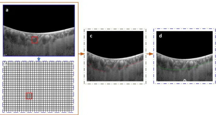
Ater training the model, it was used for the segmentation of the choroid layer. In order to segment out the choroid layer, a counter matrix was proposed. he matrix was created with the same size as the image and ini-tialized as a zero matrix. Ater each prediction of a patch in terms of its label, if the label was 1, all the pixels in the counter matrix corresponding to the patch were increased by 1. Ater inishing the prediction, the counter with the highest number in each column was chosen to it in the cubic curve for the choroid layer segmentation.
Figure 10 shows the concept of the counter matrix, where every patch was analyzed based on its label and, if the label was 1, all pixels corresponding to that patch in the counter matrix were set to the value 1. Later, in order to mark the boundary of the choroid layer, the counter having highest number in every column was selected to be it in the curve for the marking of the boundary. Figure 11 shows the comparison between the OCT image labeled by specialists and OCT image segmented by the proposed method.
the distance between the BM and the lower surface of the choroidal vasculature was calculated. Choroidal vascu-lature and BM-equivalent thickness maps were created for all subjects. he error rate between the thickness map generated by doctors and map generated by the proposed method was also calculated. Figure 12 illustrates how the thickness of choroid layer was calculated, with speciic steps described below:
• For each igure, the width was 760 pixels and the height was 456 pixels
• Next, a scaling operation was applied. We imposed 200 um maps, with 25 pixels in width and 76 pixels in height, so we could get the true thickness of each point
• here were 25 igures for each patient and the interval between two igures was 240 um
• According to steps 1–3, we could map a 25 × 760 matrix (refers to the pixel value on the igure) to 5760 um ×
6080 um (refers to the real value of patient). he thickness value would then be mapped in diferent colors in the generated map.
Experimental Analysis
[image:12.595.159.514.45.234.2]Dataset.
he data set of the ocular images used in this work was collected from Shanghai Jiao Tong University Ailiated Sixth People’s Hospital, China by using the volume scan mode with swept source OCT. he task of collecting data was undertaken in agreement with the organization’s research ethics conventions. he study was performed in accordance with the Declaration of Helsinki(DoH) and approved by the Ethics Committee of Shanghai Sixth People’s Hospital (reference: 2014-11-01). Written consent has been obtained from all subjects, and informed consent for study participation has been obtained. he data set contained 525 OCT scans from 21 healthy subjects. he images were centered at the macula region. All 21 subjects included 25 OCT scans showing diferent depths of the macula region. 275 images were used to train the network whereas 250 images were used to test the methodology. he OCT scans of each subject were uniformly selected and manually labeled along the outermost edges of the choroidal and BM boundaries. 25 OCT scans of every individual were examined using Heidelberg Eye Explorer Sotware (Heidelberg Engineering, Heidelberg, Germany).Figure 10. Counter Matrix Concept: (a and b) represents the counter matrix, (c) calculate the maximum index in each column and (d) shows the segmented choroid layer ater applying polynomial itting.
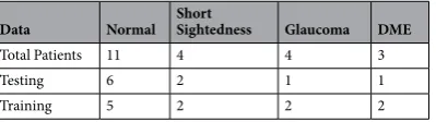
[image:12.595.161.477.289.389.2]he examined data provided (i) the automated retinal boundary for the choroidal boundary, (ii) the dots on the internal limiting membrane to the RPE boundary, and (iii) the marks on the RPE boundary to the choroidal scleral junction. Choroidal Volume (CV) was also calculated at the 6-mm circle. Out of 21 individuals, data of 11 people had normal OCT B-Scans, 4 OCT B-Scans were from individuals afected by short sightedness, 3 individ-ual’s data were afected by glaucoma and another 3 patients were sufering from mild DME. For each image, an expert ophthalmologist from Shanghai Hospital 6 manually annotated 2 boundaries (BM and the choroid layer). To overcome and reduce the manual segmentation error, two expert ophthalmologists provided the segmentation measurements of the required boundaries. Results between the two experts did not difer signiicantly (p = 0.359). he average of the two results was used in the conducted study. he manual segmentation by the experts was used as ground truth. Variation between slices (diferent depth of the choroid) was relatively small around the macula area; this interpolated ground truth was conirmed as appropriate by the experts. Table 1 can be analyzed to ana-lyze the data division for the testing and training of the method.
Ground Truth Labeling.
Images being used in this research were from real patients. Ground truth was speciied by the ophthalmologist of Shanghai Jiao Tong University Ailiated Sixth People’s Hospital. he specialist manually segmented BM and choroid layer on the OCT images. hus, these manually segmented images were used as ground truth in the proposed method. [image:13.595.103.552.49.253.2]Experimental settings.
Our algorithm was implemented in MATLAB R2016b and run on a server with a GPU of 12 with 2 GB memory, with Intel(R) Xeon(R) CPU E5-2630 v4 @ 2.20 GHz (10 cores) processor, 64 GB of RAM space and an operating system of 64 bits. Cross entropy loss function was used following a pixel-wise sot-max over the network’s inal output. he learning rate of the CNN was selected to be 0.001 for the irst 20 epochs and 0.0001 for the last 20 epochs (total of 40 epochs). he system was trained with a weight decay of 0.0005 and a momentum of 0.9. In our trials, exploring further epochs did not signiicantly reduce the training error, but instead improved computational time. Because the system was convergent ater 40 epochs, the model was not further trained. he Stochastic approximation of the gradient for the optimization was performed in mini batches of a size of 50 slices spliced from the training B-Scans with augmentation. he segmentation time for each OCT volume (25 slices) was 5 s−0.2 seconds per OCT B-scan.Figure 12. Choroid layer slices to calculate hickness Map: he thickness of each image was taken into account in order to generate the thickness map of each individual. As a result of processing each image we get a matrix representing thickness of every layer. Finally in order to get the map, matrix was resized to actual image size in order to draw the map.
Data Normal
Short
Sightedness Glaucoma DME
Total Patients 11 4 4 3
Testing 6 2 1 1
Training 5 2 2 2
[image:13.595.159.359.329.385.2]Evaluation Metrics.
In order to test the results, some error calculation matrices were used to compute the error rate on the test data set. he metric was proposed in order to calculate the average error rate in terms of pixel values i.e. the average diference between the doctor’s segmented image and the result of our proposed method. he error rate was calculated as:= →→
⁎
err A B
h w (14)
1
where →A =A12+A22++A2n, →A is the computed thickness vector, and →B is the thickness vector provided by the ophthalmologists. h and w represent the height and width of the image, respectively. Another metric was proposed to calculate the average error between the thickness map generated by doctor and the thickness map generated by the proposed methodology. he metric can be deined as:
= | − | = + ++
err A B
h where A
A A A
w (15)
w
2 1 2
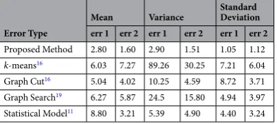
his metric was used to calculate the error rate of the proposed algorithm. Table 2 represents the average mean, variance and standard deviation calculated by the proposed methodology on the test data set. he term err1 represents the error rate between the doctor’s segmented image and segmentation performed by the pro-posed algorithm and the term err2 represents the error rate between the thickness map generated by the doctors and thickness map generated by the proposed method. Figure 13 shows the error rate computed on the test data set. Computed results are presented in Table 2.
Ater calculating the error rate, dice coeicient was also created to measure the similarity between the segmen-tation result of the proposed method and the ground truth. he dice coeicient was computed on the test data set. he coeicient was calculated as:
∩
[image:14.595.156.358.47.137.2] [image:14.595.155.359.185.303.2]= | |
| | + | |
D A B
A B
2
(16)
where A and B are the segmented choroidal region and the manually labeled choroidal region, respectively. Figure 14 shows the similarity measures observed between the manual segmentation on the test data set and segmentation performed by the proposed method. It was found that the average of the dice coeicients over 250 tested images was 97.35% with a standard deviation of 2.3%, showing good consistency between manual labeling and segmentation results of our algorithm.
Results of the proposed algorithm shows consistency with the ground truth. Observation of the manually segmented images illustrates the fact that the input points are limited and thus represents a smoother boundary whereas the proposed algorithm monitors the valley pixels more narrowly. he error rates were observed to
Error Type
Mean Variance
Standard Deviation
err 1 err 2 err 1 err 2 err 1 err 2
Proposed Method 2.80 1.60 2.90 1.51 1.05 1.12
k-means16 6.03 7.27 89.26 30.25 7.21 6.04
Graph Cut16 5.04 4.02 10.25 4.59 8.72 3.71
Graph Search19 6.27 5.87 24.5 15.80 4.94 3.97
Statistical Model11 8.80 3.21 5.39 4.90 4.40 3.24
Table 2. Mean, Variance and Standard deviation of the proposed method.
be higher when the choroidal region was thinner. hus, the similarity measurement through dice’s coeicient resulted in smaller similarity for the thinner choroid. It is notable that the manually segmented choroidal-scleral boundary is paralleled to automated segmentation. As the choroidal-scleral contains many small curvature devi-ations, specialists are required to mark surplus points as well as the corresponding boundaries. hese curvature deviations are not clearly visible unless the images are zoomed closely while performing the manual labeling. A more precise approach is adopted by the automatic segmentation through considering the small bumps and gaps present in the choroidal-scleral boundary. hus the inconsistency between the automatic and manual segmenta-tion is minimal.
he visual results of thickness map generated by our method and the doctors’ segmented images can be seen in Fig. 15. he results were then compared with other existing methods for choroid segmentation.
It is important to note that choroidal thickness measurements are highly variable in practice owing to the lack of a standardized deinition of the choroidal-scleral junction and the oten obscure imaging appearance in this region8. In our experiments, the outermost edges of the choroidal vessels are labeled as the posterior choroidal boundary and sample results of the choroid layer and BM are shown in Fig. 16.
he proposed method has been compared with other state-of-the-art methods as well. Results were computed on the test data set. he outcome of the comparison of the proposed method with a few of those state-of-the-art methods is shown in Table 3.
For further validation purposes, for each boundary segmentation, the mean signed and unsigned boundary positioning errors were compared with other algorithms such as graph cut, k-means and methods of11,19. Results are presented in Table 4 for each boundary. We implemented each of these algorithms and tested them on the test data set. In the k-means algorithm, we selected k= 3 and applied k-means algorithm on the image directly. In graph cut method, we used the result of k-means algorithm to create an initial prototype for each class and the distance between each image pixel to initial class was also calculated by k-means algorithm. he evaluation was performed on the same database and with the manually labeled ground truth. he experimental results show that the proposed method performed better than other states of art methods53–56.
[image:15.595.156.360.51.135.2]According to Table 4, observed signed border positioning errors were 0.43 ± 1.01 pixels for BM extraction and 2.80 ± 1.50 pixels for choroid segmentation, and the unsigned border positioning errors were 1.39 ± 0.25 pixels for BM extraction and 2.89 ± 1.05 pixels for choroid segmentation. Figures 17 and 18 show the mean signed and unsigned error observed on the tested data set, respectively, the signed and unsigned error were calculated with respect to the ground truth. he magnitude of signed error is much smaller than for unsigned error; hence, using signed error would misrepresent the level of deviation between the output and ground truth. herefore, the unsigned error is reported in studies as a comprehensive measure of localization errors. he errors between the proposed algorithm and the reference standard were similar to those computed between the ground truth.
Figure 14. Dice Coeicient Similarity Results: representing the segmentation result similarity of the segmented choroid layer with the ground truth on randomly selected 25 images.
[image:15.595.157.486.191.343.2]he border positioning errors of the proposed method showed signiicant improvement over other algorithms, compared in both of the tables above.
Dice coeicient similarity measures and signed and unsigned border positioning errors of the proposed technique exhibited substantial improvement over other state-of-the-art methods. Results conirmed signii-cant improvement through the proposed method. For instance, k-means and graph cut algorithm error rates are comparatively high when compared to the proposed methodology. Our method is also highly robust, overcom-ing many segmentation challenges posed by tissue anomalies such as drusen and RPE discontinuities to a large extent, and by low-quality images. his is relected in the high number of correctly segmented images and the error rate that was observed. Validation against manual tracing demonstrated that the segmentation accuracy performed at least as well as specialists.
he role of deep retinal layers in the analysis of the progression of several diseases is becoming the focus of a notable number of studies. Besides the choroidal thickness measurement, the analysis of these layers opens the door to an array of global and local retinal feature descriptors that might be associated with ocular anatomy and functioning, which are still available to be explored. hese functional and anatomical features can be highlighted with the help of precise tools for description of the choroid.
Conclusion
[image:16.595.102.554.51.216.2]In this paper, we have proposed and implemented a deep learning approach to automatically segment out the choroid layer. OCT image segmentation was carried out using morphological operations and convolutional neu-ral networks. Analysis of OCT images showed that the BM boundary is easy to extract when compared to the choroid layer, so BM was segmented irst using a series of morphological operations. he appearance of choroid
Figure 16. Sample results of BM and Choroid layer segmentation: (a) represents sample results of BM segmentation and (b) represents sample results of Choroid layer segmentation.
Method
Mean Error Rate (Choroid)
Mean Error Rate (hickness)
Ground truth vs Graph Search19. 4.19 4.62
Ground truth vs Graph Cut16 5.04 5.28
Ground truth vs k-means16 6.03 6.47
Ground truth vs Statistical Model11 8.88 10.13
Ground truth vs Proposed Method 2.80 0.65
Table 3. Mean Error Comparison of choroid layer segmentation and thickness map with other state-of-the-art methods.
Method
Signed Mean Error Rate Unsigned Mean Error Rate
BM Choroid BM Choroid
Ground truth vs Proposed Method 0.43 ± 1.01 2.8 ± 1.50 1.39 ± 0.25 2.89 ± 1.05 Ground truth vs Graph cut16 3.94 ± 0.67 40.70 ± 5.58 4.41 ± 1.79 40.50 ± 5.54
Ground truth vs k-means16 5.23 ± 2.45 −21.23 ± 10.21 6.43 ± 3.16 25.23 ± 8.72
Ground truth vs Graph Search heory19 0.59 ± 1.28 8.24 ± 4.31 3.79 ± 0.94 9.28 ± 3.21
[image:16.595.157.507.400.483.2]Ground truth vs Statistical Model11 0.78 ± 1.35 7.23 ± 4.31 2.84 ± 1.02 8.88 ± 4.40
layer is inhomogeneous, so more image statistics were required for accurate segmentation, and a CNN model was used. As the focus of this research was to analyze the health of retina based on the segmented boundaries, the thickness of segmented layers was computed to analyze the presence of retinal abnormalities. Data for real patients was used to test the results of the proposed method. he results showed an accuracy of about 97 percent. he acquired segmentation results were perceived as quite comparable to the segmentation performed by special-ists. Results showed that the proposed method maintained reduced error rates to a great extent as compared to some other existing state-of-the-art methods. To further improve the precision of the proposed method, we will work on the following related topics: improving present techniques on 2D images, improving compatibility with 3D images, optimizing parameters by considering diferent patch sizes, optimizing stride between the extracted patches, and hopefully widening the scope of the work observe other retinal abnormalities including macular edema, hypertensive retinopathy, and glaucoma.
Data Availability
he data sets generated during the study are available from the corresponding author on reasonable request.
References
1. Drexler, W. et al. Enhanced visualization of macular pathology with the use of ultrahigh-resolution optical coherence tomography.
Archives of Ophthalmology 121.5, 695–706 (2003).
2. Yonetsu, T. et al. Optical coherence tomography. Circulation Journal77(8), 1933–1940 (2013).
3. Abadia, B. et al. Choroidal thickness measured using swept-source optical coherence tomography is reduced in patients with type 2 diabetes. PloS one13(2) (2018).
4. Melancia, D. et al. Diabetic choroidopathy: a review of the current literature. Graefe’s Archive for Clinical and Experimental Ophthalmology254(8), 1453–1461 (2016).
5. Schmitt, J. M. et al. Optical coherence tomography (OCT): a review. IEEE Journal of Selected Topics in Quantum Electronics5(4), 1205–1215 (1999).
6. Puliaito, C. A. et al. Imaging of macular diseases with optical coherence tomography. Ophthalmology102(2), 217–229 (1995). 7. Fernández, D. C., Salinas, H. M. & Puliaito, C. A. Automated detection of retinal layer structures on optical coherence tomography
images. Optics Express13(25), 10200–10216 (2005).
8. Tian, J., Marziliano, P., Baskaran, M., Tun, T. A. & Aung, T. Automatic measurements of choroidal thickness in EDI-OCT images. In
Proceedings of the Annual International Conference of the IEEE Engineering in Medicine and Biology Society. 12, 5360–5363 (2012). 9. Tian, J., Marziliano, P., Baskaran, M., Tun, T. A. & Aung, T. Automatic segmentation of the choroid in enhanced depth imaging
optical coherence tomography images. Biomedical Optics Express.4(3), 397–411 (2013).
10. Zhang, L. et al. Automated segmentation of the choroid from clinical SD-OCT. Investigative Ophthalmology & Visual Science.53, 7510–7519 (2012).
11. Kaji, V. et al. Automated choroidal segmentation of 1060 nm OCT in healthy and pathologic eyes using a statistical mode. Biomedical Optics Express.3, 86–103 (2012).
12. Torzicky, T. et al. Automated measurement of choroidal thickness in the human eye by polarization sensitive optical coherence tomography. Optics Express.20, 7564–7574 (2012).
13. Duan, L., Yamanari, M. & Yasuno, Y. Automated phase retardation oriented segmentation of chorio-scleral interface by polarization sensitive optical coherence tomography. Optics Express.20, 3353–3366 (2012).
[image:17.595.159.360.46.133.2]14. Lu, H., Boonarpha, N., Kwong, M. T. & Zheng, Y. Automated segmentation of the choroid in retinal optical coherence tomography images. In Proceedings of the 35th Annual International Conference of the IEEE Engineering in Medicine and Biology Society13, 5869872 (2013).
[image:17.595.156.365.185.288.2]15. Garvin, M. K. et al. Intraretinal layer segmentation of macular optical coherence tomography images using optimal 3-D graph search. IEEE Transactions on Medical Imaging.27, 1495–1505 (2008).
16. Danesh, H., Kaieh, R., Rabbani, H. & Hajizadeh, F. Segmentation of choroidal boundary in enhanced depth imaging OCTs using a multiresolution texture based modeling in graph cuts. Computational and Mathematical Methods in Medicine (2014).
17. Haeker, M., Wu, X., Abramof, M., Kardon, R. & Sonka, M. Incorporation of regional information in optimal 3-D graph search with application for intraretinal layer segmentation of optical coherence tomography images. Biennial International Conference on Information Processing in Medical Imaging, 607–618(2007).
18. Hu, Z., Wu, X., Ouyang, Y., Ouyang, Y. & Sadda, S. R. Semiautomated segmentation of the choroid in spectral-domain optical coherence tomography volume scans. Investigative Ophthalmology and Visual Science.54(3), 1722–1729 (2013).
19. Alonso-Caneiro, D., Read, S. A. & Collins, M. J. Automatic segmentation of choroidal thickness in optical coherence tomography.
Biomedical Optics Express.4(12), 2795–2812 (2013).
20. Wang, C., Li, Y. & Wang, Y. X. Automatic choroidal layer segmentation using markov random ield and level set method. IEEE journal of Biomedical and Health Informatics (2017).
21. Rossant, F., Ghorbel, I., Bloch, I., Paques, M. & Tick, S. Automated segmentation of retinal layers in OCT imaging and derived ophthalmic measures. IEEE International Symposium on Biomedical Imaging 1370–1373 (2009).
22. Ghorbel, I., Rossant, F., Bloch, I., Tick, S. & Paques, M. Automated segmentation of macular layers in OCT images and quantitative evaluation of performances. Pattern Recognition.44(8), 1590–1603 (2011).
23. Wang, C. et al. Segmentation of intra-retinal layers in 3d optic nerve head images. International Conference on Image and Graphics
321–332 (2015).
24. Esmaeelpour, M. et al. Choroidal haller’s and sattler’s layer thickness measurement using 3-dimensional 1060-nm optical coherence tomography. PloS One.9(6), e99690 (2014).
25. Wang, C. et al. Automated layer segmentation of 3d macular images using hybrid methods. International Conference on Image and Graphics. 6(14–28) (2015).
26. CChiu, S. J. et al. Automatic segmentation of seven retinal layers in SDOCT images congruent with expert manual segmentation.
Optics Express 18.8(18), 19413–19428 (2010).
27. Kaieh, R. et al. Intra-retinal layer segmentation of 3D optical coherence tomography using coarse grained difusion map. Medical image analysis.17(8), 907–928 (2013).
28. Tolliver, D. A., Koutis, I., Ishikawa, H., Schuman, J. S. & Miller, G. L. Automatic multiple retinal layer segmentation in spectral domain OCT scans via spectral rounding. Investigative Ophthalmology & Visual Science49(13), 1878–1878 (2008).
29. Ronneberger, O., Fischer, P. & Brox, T. U-net: convolutional networks for biomedical image segmentation. Medical Image Computing and Computer-Assisted Intervention 234–241 (2015).
30. Li, Z., Wang, Y., Yu, J., Guo, Y. & Cao, W. Deep Learning based Radiomics (DLR) and its usage in noninvasive IDH1 prediction for low grade glioma. Scientiic reports.7(1), 5467 (2017).
31. Ghafoorian, M. et al. Location sensitive deep convolutional neural networks for segmentation of white matter hyperintensities.
Scientiic Reports.7(1), 5110 (2017).
32. Tu, X. et al. Automatic Categorization and Scoring of Solid, Part-Solid and Non-Solid Pulmonary Nodules in CT Images with Convolutional Neural Network. Scientiic Reports.7(1), 8533 (2017).
33. Zhang. et al. Deep convolutional neural networks for multi-modality isointense infant brain image segmentation. NeuroImage.108, 214–224 (2015).
34. Havaei, M. et al. Brain tumor segmentation with deep neural networks. Medical Image Analysis.35, 18–31 (2017).
35. Trebeschi, S. et al. Deep learning for fully-automated localization and segmentation of rectal cancer on multiparametric MR.
Scientiic reports.7(1), 5301 (2017).
36. Sharma, K. et al. Automatic segmentation of kidneys using deep learning for total kidney volume quantiication in autosomal dominant polycystic kidney disease. Scientiic reports.7(1), 2049 (2017).
37. Kenny, C. H. et al. Urinary bladder segmentation in CT urography using deep learning convolutional neural network and level sets.
Medical Physics 43.4, 1882–1896 (2016).
38. Hong, T. J. et al. Segmentation of optic disc, fovea and retinal vasculature using a single convolutional neural network. Journal of Computational Science.20, 70–79 (2017).
39. Liskowski, P. & Krawiec, K. Segmenting retinal blood vessels with deep neural networks. IEEE Transactions on Medical Imaging. 35
(2016).
40. Ngo, L., Han, J. H. Advanced deep learning for blood vessel segmentation in retinal fundus images. Brain-Computer Interface, 5th International Winter Conference 91–92 (2017).
41. Dasgupta, A., Singh, S. A. Fully convolutional neural network based structured prediction approach towards the retinal vessel segmentation. Biomedical Imaging, IEEE 14th International Symposium 248–251 (2017).
42. Dhoot, D. S. et al. Evaluation of choroidal thickness in retinitis pigmentosa using enhanced depth imaging optical coherence tomography. British Journal of Ophthalmology.97, 66–69 (2013).
43. Imamura, Y., Fujiwara, T., Margolis, R. & Spaide, R. F. Enhanced depth imaging optical coherence tomography of the choroid in central serous chorioretinopathy. Retina.29, 1469–1473 (2009).
44. Manjunath, V., Goren, T., Fujimoto, T. G. & Duker, J. S. Analysis of choroidal thickness in age-related macular degeneration using spectral-domain optical coherence tomography. RAm. Journal of Ophthalmology.4, 663–668 (2011).
45. Esmaeelpour, M. et al. Mapping choroidal and retinal thickness variation in type 2 diabetes using three-dimensional 1060-nm optical coherence tomography. Investigative Ophthalmology and Visual Science.8, 5311–5316 (2011).
46. Sim, D. A. et al. Repeatability and reproducibility of choroidal vessel layer measurements in diabetic retinopathy using enhanced depth optical coherence tomography. Investigative Ophthalmology and Visual Science.4, 2893–2901 (2013).
47. Gopinath, K., Rangrej, S. B. & Sivaswamy, J. A deep learning framework for segmentation of retinal layers from OCT images. 48. Pekala, M. et al. Deep Learning based Retinal OCT Segmentation. arXiv preprint arXiv, 801.09749 (2018).
49. Fang, L. et al. Automatic segmentation of nine retinal layer boundaries in OCT images of non-exudative AMD patients using deep learning and graph search. Biomedical optics express8(5), 2732–2744 (2017).
50. Roy, A. G. et al. ReLayNet: retinal layer and luid segmentation of macular optical coherence tomography using fully convolutional networks. Biomedical optics express8(8), 3627–3642 (2017).
51. Jia, Y. et al. Cafe: Convolutional Architecture for Fast Feature Embedding. arXiv preprint arXiv, 1408.5093 (2014). 52. Krizhevsky, A. & Hinton, G. Convolutional deep belief networks on cifar-10. Unpublished manuscript40, 7 (2010).
53. Giani, A. et al. Artifacts in automatic retinal segmentation using diferent optical coherence tomography instruments. Retina.30(4), 607–6164 (2010).
54. Zhang, L. Automated segmentation and analysis of layers and structures of human posterior eye. he University of Iowa (2015). 55. Vuong, V. S. et al. Repeatability of choroidal thickness measurements on enhanced depth imaging optical coherence tomography
using diferent posterior boundaries. American Journal of Ophthalmology169, 104–112 (2016).
Author Contributions
S.M. designed the study, performed experiments and wrote the manuscript. P.L. and B.S. helped to design the study and the experiments and supervised the project. H.L., X.W., P.Y., and Q.W. provided the dataset and the manual annotations. R.F., A.M., J.Q., and W.J. provided comments and feedback on the study and the results. All the authors reviewed the manuscript.
Additional Information
Supplementary information accompanies this paper at https://doi.org/10.1038/s41598-019-39795-x.
Competing Interests: he authors declare no competing interests.
Publisher’s note: Springer Nature remains neutral with regard to jurisdictional claims in published maps and institutional ailiations.
Open Access This article is licensed under a Creative Commons Attribution 4.0 International License, which permits use, sharing, adaptation, distribution and reproduction in any medium or format, as long as you give appropriate credit to the original author(s) and the source, provide a link to the Cre-ative Commons license, and indicate if changes were made. he images or other third party material in this article are included in the article’s Creative Commons license, unless indicated otherwise in a credit line to the material. If material is not included in the article’s Creative Commons license and your intended use is not per-mitted by statutory regulation or exceeds the perper-mitted use, you will need to obtain permission directly from the copyright holder. To view a copy of this license, visit http://creativecommons.org/licenses/by/4.0/.